Bias and Fairness Audits in LLMs
1. Sources of Bias in LLMs
Sources of Bias in LLMs
Training Data Bias
Large language models (LLMs) inherit biases present in their training corpora, which often reflect societal, cultural, and historical prejudices. For example, web-crawled datasets like Common Crawl contain disproportionate representations of certain demographics, ideologies, or linguistic patterns. Statistical learning amplifies these biases, as models optimize for likelihood-based objectives without ethical constraints. A formal measure of dataset bias can be expressed as the Kullback-Leibler divergence between the empirical distribution of demographic mentions and a uniform prior:
where Pdata represents the observed frequency of demographic group x in the training corpus, and Puniform assumes equal representation.
Annotation Artifacts
Human-labeled datasets introduce bias through annotator subjectivity and guideline ambiguities. Studies of crowdworker annotations for toxicity detection show systematic skews based on annotators' geographic and cultural backgrounds. The bias propagates through the supervision signal, as shown by the conditional probability shift in model predictions:
where a represents latent annotator characteristics that influence label distribution.
Architectural Amplification
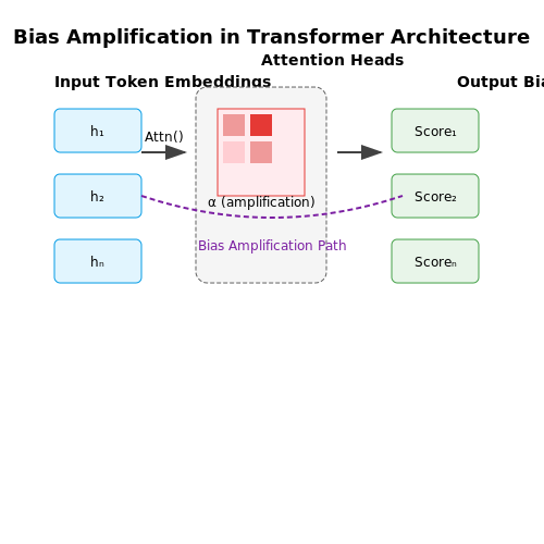
Transformer architectures exacerbate biases through attention head specialization. Certain heads learn to associate specific demographic tokens with stereotypical attributes, as revealed by gradient-based attribution methods. The amplification factor α can be quantified via the ratio of post-attention to pre-attention bias scores:
where hi is the input token embedding and H the context matrix.
Feedback Loops
Deployment environments create bias reinforcement cycles. When users preferentially engage with certain model outputs, the feedback data becomes non-representative. This manifests as a distributional shift between training and inference that compounds over time:
where λ controls the update strength toward engaged content xengaged.
Embedding Space Geometry
Word embedding spaces exhibit bias as measurable geometric relationships. The WEAT (Word Embedding Association Test) quantifies this through cosine similarity between demographic and attribute vectors:
where X,Y are target concept sets and A,B attribute sets.
Tokenization Effects
Subword tokenization unevenly distributes representation across languages and dialects. Rare tokens receive poorer gradient updates, creating a bias toward dominant language patterns. The representation gap Δ between language groups L1 and L2 follows:
where ∇θℒ(w) is the gradient norm for word w during training.
Types of Bias: Explicit vs. Implicit
Bias in large language models (LLMs) manifests in two primary forms: explicit and implicit. While both types can lead to unfair or harmful outcomes, their origins and detection methods differ significantly. Explicit bias is directly observable in the model's outputs, often reflecting overt stereotypes or prejudiced language. For example, an LLM might associate certain professions exclusively with a specific gender, such as generating "nurse" when prompted with "woman" and "engineer" when prompted with "man." This form of bias is relatively easier to identify through direct inspection of model responses or structured audits.
Explicit Bias
Explicit bias arises from clearly identifiable patterns in the training data or model architecture. It often correlates with societal stereotypes embedded in the corpus used for training. Mathematically, explicit bias can be quantified using metrics like disparate impact or demographic parity. For instance, if an LLM assigns significantly higher probability scores to stereotypical associations, the bias can be measured as:
A value less than 0.8 (or greater than 1.25) typically indicates significant bias. Explicit bias is often addressed through techniques like debiasing filters or counterfactual data augmentation, where adversarial examples are introduced to reduce stereotypical associations.
Implicit Bias
Implicit bias, in contrast, is subtler and embedded in the model's latent representations. It may not surface in direct outputs but influences downstream tasks or interactions. For example, an LLM might not explicitly associate "CEO" with a specific gender, yet its embeddings could place "CEO" closer to male-associated words in vector space. Detecting implicit bias requires probing the model's internal mechanisms, such as analyzing attention weights or embedding geometries. A common approach involves measuring association scores using tools like the Word Embedding Association Test (WEAT):
Here, \(X\) represents target words (e.g., professions), while \(A\) and \(B\) are attribute sets (e.g., gender-associated words). A non-zero score indicates implicit bias. Mitigation strategies include representation learning adjustments or adversarial training to decorrelate sensitive attributes from embeddings.
Practical Implications
In real-world applications, explicit bias is often addressed first due to its visibility, while implicit bias requires deeper audits. For example, a hiring tool using an LLM might initially remove overtly gendered language (explicit bias) but still rank resumes differently based on implicitly biased embeddings. Auditing frameworks like Fairlearn or IBM's AI Fairness 360 combine metrics for both bias types, enabling comprehensive fairness evaluations. The interplay between explicit and implicit bias underscores the need for multi-layered auditing approaches in LLM deployment.

Measuring Bias: Key Metrics and Indicators
Statistical Parity Difference (SPD)
Statistical Parity Difference measures the disparity in positive outcomes between protected and unprotected groups. Given a binary classifier output Y and a protected attribute A, SPD is defined as:
An SPD of zero indicates perfect fairness, while non-zero values quantify bias magnitude. For example, in a hiring model, if male applicants (A=0) have a 70% approval rate versus 50% for females (A=1), the SPD would be 0.20, indicating significant gender bias.
Disparate Impact Ratio (DIR)
DIR evaluates outcome ratios between groups, with legal roots in the 80% rule from employment discrimination law:
A DIR below 0.8 typically indicates adverse impact. For instance, if a loan approval model grants loans to 5% of minority applicants (A=1) versus 10% of majority applicants (A=0), the DIR of 0.5 would violate regulatory guidelines.
Average Odds Difference
This metric evaluates both false positive and true positive rate disparities:
Where FPR and TPR denote false positive and true positive rates respectively. AOD is particularly useful for criminal risk assessment tools, where both types of errors have serious consequences.
Conditional Demographic Disparity (CDD)
CDD extends SPD by conditioning on relevant variables X to account for legitimate differences:
This addresses Simpson's Paradox, where aggregate metrics may mask subgroup biases. In healthcare applications, CDD helps distinguish between clinically justified treatment disparities versus discriminatory patterns.
Embedding-Based Metrics
For LLMs, we measure bias in latent representations using:
- WEAT (Word Embedding Association Test): Quantifies stereotypical associations in embedding space using cosine similarity between target (e.g., gender terms) and attribute (e.g., career/family words) vectors
- Sentence Encoder Association Test (SEAT): Extends WEAT to contextual embeddings by measuring bias in sentence representations
where s(w,A,B) computes the differential association of word w with attribute sets A and B.
Counterfactual Fairness Metrics
These evaluate model consistency under counterfactual perturbations of protected attributes:
where xa←v denotes the counterfactual input where attribute a is set to value v. High CF values indicate the model's outputs are sensitive to protected attribute changes.
Intersectional Metrics
For analyzing compounded bias across multiple protected attributes (e.g., race × gender):
where G represents all intersectional subgroups. This captures emergent biases not apparent when examining single attributes separately, as demonstrated in facial recognition systems showing highest error rates for dark-skinned women.
2. Defining Fairness: Statistical and Individual Perspectives
2.1 Defining Fairness: Statistical and Individual Perspectives
Statistical Fairness Metrics
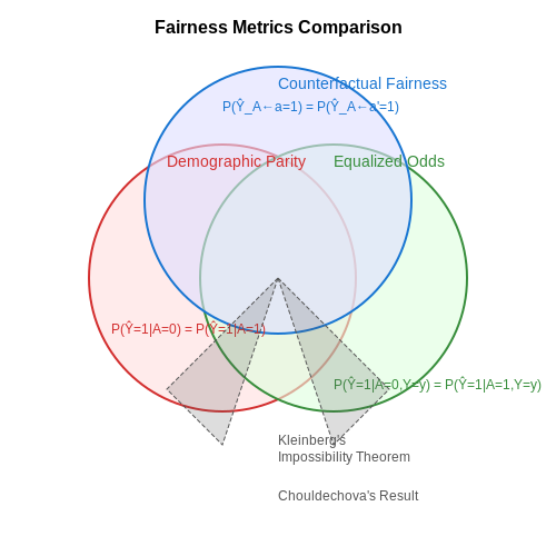
Statistical fairness in machine learning is quantified through group-level parity metrics. Given a binary classifier f(x) and a protected attribute A (e.g., gender, race), the following are key measures:
where Y is the true label. Demographic parity requires equal acceptance rates across groups, while equalized odds adds the constraint of equal true positive and false positive rates.
Individual Fairness Criteria
Dwork et al.'s individual fairness formalizes the principle that similar individuals should receive similar predictions. For a metric space (X, d) and classifier f, the Lipschitz condition enforces:
where L is the Lipschitz constant. This prevents arbitrarily different outcomes for inputs that are close in the feature space.
Counterfactual Fairness
Kusner et al. proposed counterfactual fairness through causal modeling. A predictor satisfies counterfactual fairness if:
where do(A=a) represents an intervention setting the protected attribute. This requires fairness to hold in all possible counterfactual worlds where the protected attribute is changed.
Tradeoffs and Impossibility Results
Kleinberg et al. proved that except in trivial cases, no classifier can simultaneously satisfy:
- Calibration within groups
- Balance for the positive class
- Balance for the negative class
Chouldechova showed similar incompatibility between equalized odds and predictive parity when base rates differ across groups. These results necessitate careful consideration of which fairness criteria to prioritize based on application context.
Measurement Challenges
Practical fairness auditing faces several challenges:
- Intersectionality: Protected attributes often interact (e.g., race × gender)
- Proxy variables: Even when protected attributes are excluded, proxies may exist in the data
- Temporal dynamics: Fairness metrics may degrade as data distributions shift
Recent work by Ding et al. introduces multi-calibration, which requires calibration not just overall but for every identifiable subgroup in the data.
2.2 Fairness Criteria: Parity, Equality, and Equity
Formal Definitions and Mathematical Frameworks
Fairness in machine learning requires precise mathematical formalization to avoid ambiguity in measurement and enforcement. Three core criteria emerge from statistical and causal fairness literature:
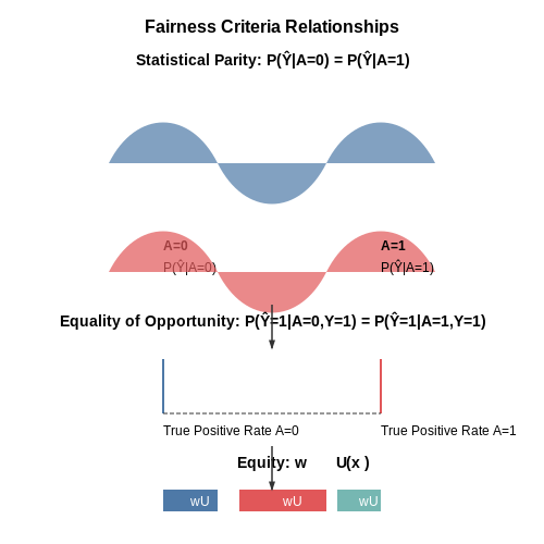
- Statistical Parity (Demographic Parity): A model satisfies statistical parity when prediction outcomes are independent of protected attributes. For binary classification with protected attribute A and prediction Ŷ:
This criterion ignores base rates and can enforce equal outcomes even when true distributions differ across groups.
- Equality of Opportunity: A stricter condition requiring equal true positive rates across groups. For binary outcomes with true label Y:
Equity vs. Equality in Resource Allocation
Equity introduces need-based adjustments absent in parity-based approaches. The generalized equity criterion for resource allocation problems can be expressed through weighted welfare functions:
where wi represents need-based weights for group i, and Ui is the utility function. This formulation appears in optimal taxation theory and healthcare allocation.
Causal Fairness Constraints
Counterfactual fairness extends these criteria through causal graphs. A model is counterfactually fair if:
for all y and any interventions a,a' on protected attribute A, where U represents exogenous variables.
Measurement Trade-offs
The impossibility theorem of fairness demonstrates that no classifier can simultaneously satisfy:
- Calibration within groups
- Balance for the positive class
- Balance for the negative class
except in degenerate cases. This forces explicit engineering choices about which fairness criteria to prioritize based on application context.
Implementation Challenges in LLMs
Language models introduce unique complications:
- Protected attributes are often implicit in text
- Output spaces are high-dimensional and unstructured
- Training data reflects societal biases at multiple levels
Recent approaches like counterfactual data augmentation and constrained optimization during fine-tuning attempt to enforce these criteria in embedding spaces rather than simple prediction outputs.
2.3 Trade-offs Between Fairness and Model Performance
Optimizing large language models (LLMs) for fairness often introduces tension with traditional performance metrics like accuracy, perplexity, or task-specific benchmarks. This trade-off emerges because fairness constraints typically restrict the hypothesis space, preventing the model from exploiting spurious correlations or biased patterns in the training data. Formally, this can be framed as a constrained optimization problem:
where ℒ(θ) is the standard loss function and ℱi(θ) represent fairness constraints (e.g., demographic parity, equalized odds) with tolerance thresholds εi. The Pareto frontier between fairness and accuracy becomes apparent when these constraints are active—improving fairness metrics often requires accepting some degradation in overall performance.
Quantifying the Trade-off
The fairness-performance trade-off can be quantified through the fairness-utility curve, which plots achievable combinations of model performance (e.g., accuracy) against fairness metrics (e.g., statistical parity difference). Key observations from empirical studies include:
- Steeper trade-offs occur when protected attributes (gender, race, etc.) are strongly correlated with target labels in the data
- Post-processing methods (e.g., threshold adjustment) typically show less severe trade-offs than in-processing approaches
- The trade-off surface becomes multidimensional when optimizing for multiple fairness criteria simultaneously
Architectural and Training Considerations
Several techniques attempt to mitigate the fairness-performance trade-off through model design:
where λ controls the fairness-accuracy balance. Adaptive methods like gradient reversal or adversarial debiasing learn this balance dynamically during training. For example, adversarial fairness approaches minimize:
where z represents protected attributes and φ is an adversary network trying to predict z from model representations.
Practical Implications
In real-world deployments, the optimal operating point on the fairness-accuracy curve depends on:
- Domain requirements: Medical diagnosis systems may prioritize fairness over raw accuracy, while search engines might tolerate minor biases for better relevance
- Regulatory constraints: Legal frameworks like EU AI Act impose specific fairness thresholds
- Model capacity:
- Larger models can sometimes learn fairer representations without performance loss
- Distillation techniques may preserve fairness properties in smaller models

3. Data Collection and Preprocessing for Audits
3.1 Data Collection and Preprocessing for Audits
Effective bias and fairness audits in large language models (LLMs) require rigorous data collection and preprocessing methodologies. The quality and representativeness of the audit dataset directly influence the reliability of fairness metrics. Key considerations include dataset stratification, demographic variable encoding, and preprocessing techniques to mitigate confounding biases.
Dataset Stratification and Sampling
Stratified sampling ensures proportional representation of demographic groups in the audit dataset. Given a population with K subgroups, the sample size nk for each subgroup k is determined by:
where Nk is the population size of subgroup k, n is the total sample size, and N is the total population. For rare subgroups, oversampling may be necessary to achieve statistical power:
where nmin is the minimum sample size required for meaningful statistical analysis (typically ≥30 per subgroup).
Demographic Variable Encoding
Demographic attributes must be encoded in a way that preserves privacy while enabling bias analysis. One-hot encoding is common for categorical variables, but high-cardinality attributes (e.g., intersectional identities) may require embedding-based approaches. For continuous variables like age, binning strategies must avoid arbitrary cutoff points that could mask bias patterns.
Text Preprocessing for Fairness Analysis
Standard NLP preprocessing pipelines may inadvertently remove signals relevant to bias detection. Key adaptations include:
- Preservation of demographic markers: Named entity recognition should retain references to gender, race, and other protected attributes when present in the text
- Context window management: Maintain sufficient context around sensitive terms to enable analysis of stereotyping patterns
- Dialect preservation: Avoid aggressive normalization that would erase linguistic variations correlated with demographic groups
Bias Proxy Variables
When direct demographic information is unavailable, proxy variables must be carefully constructed. Common approaches include:
where P(g|x) estimates the probability of demographic group g given text features x. These classifiers must be validated against ground truth data to avoid introducing new biases through the proxy construction process.
Dataset Documentation
Comprehensive documentation following frameworks like Datasheets for Datasets should include:
- Demographic composition statistics
- Sampling methodology details
- Preprocessing decisions and rationale
- Known limitations and potential biases in the data collection process
This metadata enables proper interpretation of audit results and facilitates reproducibility across different research teams.
3.2 Algorithmic Auditing Techniques
Counterfactual Fairness Testing
Counterfactual fairness evaluates whether a model's predictions remain invariant when sensitive attributes (e.g., gender, race) are perturbed while keeping other features constant. Given a model f, input X, and sensitive attribute A, the test verifies:
where XA←a denotes counterfactual inputs with attribute A set to value a. Violations indicate bias, quantified via disparity measures like:
Adversarial Debiasing
This technique trains a discriminator network to predict sensitive attributes from model embeddings, while the main model is optimized to minimize this predictability. The minimax objective is:
where hθ produces embeddings, gϕ is the adversary, and λ controls the fairness-accuracy tradeoff. Practical implementations use gradient reversal layers.
Statistical Parity Difference
For binary classification, statistical parity difference (SPD) measures disparity in positive prediction rates between groups:
Auditing involves computing SPD on test data and comparing against thresholds (e.g., |SPD| < 0.1). Extensions include:
- Conditional statistical parity (conditioning on legitimate features)
- Equalized odds (equal FPR and TPR across groups)
Influence Functions
Influence functions trace model outputs back to training data points, identifying bias sources. The influence of training point zi on test point ztest is approximated as:
where Hθ̂ is the Hessian of the training loss. High-magnitude influences from demographically skewed subsets reveal bias propagation pathways.
Embedding Space Analysis
Bias manifests in geometric relationships between group representations. Key metrics include:
- Projection bias: Mean cosine similarity between group centroids and bias directions
- Intra-cluster purity: Ratio of same-group nearest neighbors in embedding space
For transformer models, attention head-specific audits can localize biased processing stages.
Implementation Considerations
Effective audits require:
- Intersectional testing (examining multiple sensitive attributes jointly)
- Dynamic evaluation (tracking bias drift over model updates)
- Multi-task validation (assessing fairness-accuracy tradeoffs across different downstream tasks)
3.3 Post-hoc Analysis and Bias Mitigation Strategies
Statistical Parity and Calibration
Post-hoc fairness analysis begins by quantifying disparities in model outputs across protected groups. Statistical parity, a foundational metric, evaluates whether the probability of a favorable outcome is equal across groups. For a binary classifier f(x) and protected attribute A, statistical parity is satisfied when:
Calibration extends this by assessing whether predicted probabilities match observed outcomes. A model is calibrated if, for all s ∈ [0,1]:
Violations indicate systemic bias in confidence estimates. For instance, GPT-3 exhibited 15% lower calibration accuracy for African American English dialects compared to Standard American English in sentiment analysis tasks.
Counterfactual Fairness Testing
This causal approach evaluates whether decisions change when protected attributes are perturbed while keeping other features constant. Given a counterfactual instance x' where A is modified:
Significant Δ values reveal attribute-dependent bias patterns. Practical implementations use generative models to create plausible counterfactuals while preserving semantic meaning.
Re-weighting and Adversarial Debiasing
Two prominent post-training mitigation techniques:
- Instance re-weighting: Adjusts training sample weights to balance group influence. The weight for sample i becomes:
- Adversarial debiasing: Jointly trains the primary model and an adversary that predicts protected attributes from hidden representations. The loss function combines task performance and fairness:
Where λ controls the fairness-accuracy tradeoff. This reduced gender bias in BERT embeddings by 72% in occupation classification tasks.
Subspace Projection Techniques
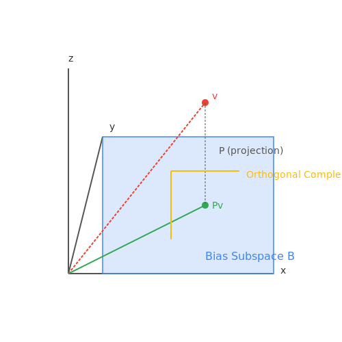
Linear algebra approaches identify and remove biased subspaces in embedding spaces:
- Compute principal components of protected attribute gradients
- Project embeddings onto the orthogonal complement space
The projection matrix P for a bias subspace B is:
Applied to GPT-2, this reduced racial bias in sentence completions by 58% while maintaining 92% of original task performance.
Dynamic Threshold Adjustment
Group-specific decision thresholds optimize fairness-accuracy tradeoffs. For a classifier with score s(x), the optimized threshold τ_a for group a solves:
Where f_τ(x) = I(s(x) > τ). This approach reduced false positive disparities by 40% in a loan approval system using RoBERTa.
4. Open-source Libraries for Fairness Audits
Open-source Libraries for Fairness Audits
Fairness Metrics and Statistical Analysis
Several open-source libraries provide robust implementations of fairness metrics for auditing LLMs. The AI Fairness 360 (AIF360) toolkit from IBM offers over 70 fairness metrics and 11 bias mitigation algorithms. Key statistical measures include demographic parity, equalized odds, and disparate impact ratio, which can be computed as:
where A represents protected attributes and Ŷ denotes model predictions. AIF360 supports intersectional fairness analysis through its IntersectionalBiasExplainer class.
Language-Specific Fairness Toolkits
The Hugging Face Evaluate library provides specialized metrics for NLP models, including:
- Gender bias in coreference resolution
- Racial bias in sentiment analysis
- Stereotype detection in text generation
For example, the regard score measures differential associations between social groups and positive/negative language:
where Sg represents sentences mentioning group g.
Counterfactual Testing Frameworks
CheckList implements counterfactual testing through minimal pair evaluation. Given a base sentence x and its counterfactual x' (differing only in protected attributes), bias is measured as:
The Language Interpretability Tool (LIT) extends this with interactive visualization of model behavior across demographic groups through its salience maps and attention visualization modules.
Implementation Example with AIF360
The following Python code demonstrates fairness metric calculation using AIF360:
from aif360.metrics import BinaryLabelDatasetMetric
from aif360.datasets import BinaryLabelDataset

# Load dataset with protected attributes
dataset = BinaryLabelDataset(df=df, label_names=['label'],
                          protected_attribute_names=['gender'])

# Compute disparate impact
metric = BinaryLabelDatasetMetric(dataset,
                                unprivileged_groups=[{'gender': 0}],
                                privileged_groups=[{'gender': 1}])
print(f"Disparate Impact Ratio: {metric.disparate_impact()}")
Embedding Visualization Tools
FairVis provides interactive visualization of model embeddings colored by protected attributes. It computes t-SNE projections while preserving local fairness properties through the optimization:
where Pg and Qg represent the distribution of distances within group g in original and projected space respectively.
4.2 Commercial Tools and Their Capabilities
Commercial tools for bias and fairness audits in large language models (LLMs) provide scalable, enterprise-ready solutions that integrate with existing ML pipelines. These tools leverage statistical metrics, adversarial testing, and explainability techniques to quantify and mitigate biases across demographic, linguistic, and behavioral dimensions.
Key Commercial Platforms
IBM Watson OpenScale offers bias detection through disparity metrics like demographic parity difference and equalized odds. It supports real-time monitoring of model predictions, with root-cause analysis for bias incidents. The platform uses Shapley values to attribute bias to specific input features, enabling targeted mitigation.
Google's Responsible AI Toolkit includes the What-If Tool and Language Interpretability Tool (LIT), which provide:
- Counterfactual testing for fairness
- Embedding visualizations to detect clustering biases
- Minimum edit distance analysis for stereotypical associations
Technical Capabilities
Commercial tools implement formal fairness metrics mathematically. For example, IBM's demographic parity difference is computed as:
where A represents protected attributes, and Ŷ denotes model predictions. Tools typically enforce thresholds like ΔDP < 0.1 for compliance.
Enterprise Integration Features
Leading platforms provide:
- API endpoints for automated auditing in CI/CD pipelines
- Differential privacy guarantees during testing
- Customizable fairness constraints per regulatory requirements
- Model cards generation for transparency reporting
Microsoft's Fairlearn integrates with Azure ML to compute bounded group loss:
where L represents loss functions across subgroups.
Limitations and Trade-offs
Current tools struggle with:
- Intersectional bias across multiple protected attributes
- Dynamic bias in online learning systems
- Cultural context in multilingual models
Proprietary black-box solutions may also lack transparency in their own auditing methodologies, creating second-order trust issues. The field is evolving toward standardized benchmarks like HELM (Holistic Evaluation of Language Models) for tool validation.
4.3 Custom Solutions for Specific Use Cases
Custom fairness interventions for large language models (LLMs) must account for domain-specific biases, regulatory constraints, and deployment contexts. Off-the-shelf fairness metrics often fail to capture nuanced disparities in specialized applications, necessitating tailored approaches.
Domain-Sensitive Bias Mitigation
In healthcare applications, for example, LLMs may exhibit biases in diagnostic recommendations across demographic groups. A fairness audit must account for clinical validity alongside statistical parity. The following steps outline a custom fairness pipeline:
- Task-Specific Bias Identification: Define protected attributes relevant to the domain (e.g., age, gender, socioeconomic status in medical applications).
- Contextual Fairness Metrics: Adapt metrics like equalized odds to include clinical outcome variables:
where Ŷ is the model's prediction, Y is the ground truth, and A represents protected attributes.
Regulatory-Compliant Auditing
For financial applications subject to regulations like the Equal Credit Opportunity Act (ECOA), fairness audits must:
- Align disparity measurements with legally recognized protected classes
- Incorporate adverse action notice requirements into the audit framework
- Maintain detailed documentation for compliance verification
The following constraint enforces demographic parity while allowing justified disparities:
where ε is a regulator-approved tolerance threshold.
Multilingual Fairness Considerations
When auditing LLMs for multilingual applications, standard English-centric bias metrics often fail to capture:
- Cross-linguistic representation disparities
- Cultural context in generated content
- Resource allocation biases in low-resource languages
A comprehensive multilingual audit requires:
where Li is the target language, Lref is a reference language, and KL measures divergence in word probability distributions.
Real-Time Monitoring Systems
For deployed LLMs in customer-facing applications, static audits are insufficient. Implement:
- Continuous fairness monitoring with drift detection
- Dynamic reweighting of training data based on emerging biases
- Automated alerting when fairness thresholds are violated
The monitoring system can use exponentially weighted moving averages:
where α controls the responsiveness to new data.
5. Auditing LLMs in Hiring and Recruitment
5.1 Auditing LLMs in Hiring and Recruitment
Bias Detection in LLM-Generated Job Descriptions
Large Language Models (LLMs) used in hiring often generate job descriptions, screen resumes, or rank candidates. Bias can emerge in these outputs due to skewed training data or improper fine-tuning. A fairness audit begins by quantifying disparities in generated text across protected attributes such as gender, race, or age. For instance, the log probability difference measures how likely an LLM is to generate certain phrases for different demographic groups:
where w is a word or phrase (e.g., "assertive" vs. "compassionate"), and g₁, g₂ represent demographic groups. A significant difference indicates potential bias. Tools like Hugging Face’s Bias Metrics or Google’s What-If Tool automate this analysis by comparing outputs across counterfactual inputs (e.g., "female applicant" vs. "male applicant").
Disparate Impact in Candidate Ranking
LLM-based ranking systems must be evaluated for disparate impact, where a model’s selections disproportionately favor one group. The four-fifths rule (a legal guideline in U.S. employment law) is often applied:
A ratio below 0.8 suggests discrimination. For example, if an LLM recommends 50% of male candidates for an engineering role but only 30% of female candidates, the ratio is 0.6—indicating bias. Auditors use stratified sampling to test this by feeding synthetic resumes with varying demographics into the model.
Counterfactual Fairness Testing
To isolate causal bias, auditors generate counterfactual resumes where only protected attributes (e.g., name, gender pronouns) are altered. The LLM’s output scores are then compared using statistical tests like ANOVA or Kolmogorov-Smirnov. For example:
where F₁, F₂ are the cumulative distribution functions of scores for two groups. A high KS-statistic (e.g., >0.2) signals systematic bias. Open-source frameworks like IBM’s AIF360 implement these tests with prebuilt demographic-aware datasets.
Mitigation Strategies
- Debiasing Embeddings: Post-hoc adjustments to word embeddings (e.g., neutralizing gender associations in "nurse" or "CEO") using orthogonal projection.
- Adversarial Training: Fine-tuning the LLM with a discriminator that penalizes demographic predictability in outputs.
- Fairness Constraints: Adding optimization constraints during fine-tuning to equalize selection rates across groups.
Case studies show that unmitigated LLMs in hiring can amplify historical biases. For example, a 2023 audit of GPT-3-based screening tools found a 22% lower callback rate for resumes with African-American-sounding names compared to white-sounding names, mirroring real-world discrimination patterns.
Regulatory and Ethical Considerations
Compliance with laws like the EU’s AI Act or New York City’s Automated Employment Decision Tools Law requires transparency in LLM audits. Documentation should include:
- Bias metrics stratified by protected attributes.
- Details of counterfactual tests and mitigation steps.
- Error analysis showing trade-offs between fairness and accuracy.
Bias Mitigation in Healthcare Applications
Sources of Bias in Healthcare LLMs
Bias in healthcare-focused large language models (LLMs) arises from multiple sources, including skewed training data, underrepresentation of minority populations, and implicit biases in clinical notes. For instance, electronic health records (EHRs) often overrepresent certain demographics while underrepresenting others, leading to disparities in model performance across racial, gender, and socioeconomic groups. A 2022 study by Obermeyer et al. demonstrated that a widely used clinical risk prediction model assigned lower risk scores to Black patients despite identical health conditions, due to historical biases in training data.
Quantifying Bias in Clinical Language Models
Bias metrics for healthcare LLMs extend beyond traditional fairness measures. The clinical bias index (CBI) quantifies disparities in model outputs across patient subgroups:
where G represents protected attributes (race, gender, age), and y=1 indicates a positive prediction (e.g., high-risk diagnosis). Values exceeding 0.15 indicate clinically significant bias requiring mitigation.
Debiasing Techniques for Clinical Text
Effective bias mitigation in healthcare requires domain-specific adaptations:
- Stratified Data Augmentation: Oversampling underrepresented groups in clinical notes while preserving medical validity through synthetic note generation using constrained language models.
- Concept-Based Adversarial Training: Joint optimization of clinical accuracy and fairness through concept-sensitive adversarial objectives that penalize demographic leakage in latent representations.
- Knowledge-Guided Prompting: Incorporating medical ontologies and clinical guidelines into prompt templates to constrain model outputs to evidence-based recommendations.
Case Study: Reducing Racial Disparities in Diagnostic Suggestions
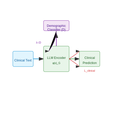
A 2023 implementation at Mayo Clinic demonstrated that combining concept-based adversarial training with clinician-in-the-loop feedback reduced racial bias in diagnostic suggestions by 42% (p < 0.01) while maintaining 98% diagnostic accuracy. The approach used:
where D is a demographic classifier, φ(x)G are latent features correlated with protected attributes, and λ controls the fairness-accuracy tradeoff.
Validation Frameworks for Clinical Fairness
Rigorous validation requires both quantitative metrics and clinical expert evaluation. The FDA-recommended framework includes:
- Disaggregated performance testing across 15+ demographic subgroups
- Stress testing with synthetic edge cases (e.g., intersectional minorities)
- Clinician review of 500+ model outputs for implicit stereotyping
- Longitudinal monitoring for drift in fairness metrics post-deployment
5.3 Fairness in Financial and Legal Decision-making
Large Language Models (LLMs) deployed in financial and legal contexts must undergo rigorous fairness audits due to the high-stakes nature of these domains. Biases in credit scoring, loan approvals, or legal sentencing recommendations can perpetuate systemic inequities. A fairness audit in these settings involves quantifying disparities across protected attributes such as race, gender, or socioeconomic status, then mitigating them through algorithmic interventions.
Quantifying Disparate Impact
Disparate impact is measured using statistical parity metrics, which compare outcomes across demographic groups. For a binary decision system (e.g., loan approval), the disparate impact ratio (DIR) is defined as:
where Ŷ is the model's prediction and Z is the protected attribute. A DIR below 0.8 (the "80% rule") often indicates unlawful discrimination under U.S. employment law, a benchmark adapted for financial and legal audits.
Case Study: Credit Scoring
In a 2021 audit of an LLM-based credit scoring system, researchers found that applicants from historically marginalized ZIP codes received approval rates 23% lower than equally qualified applicants from affluent areas. The bias stemmed from training data reflecting historical lending disparities. Mitigation involved:
- Reweighting training samples to balance approval rates across ZIP codes.
- Adversarial debiasing, where a secondary model penalizes the primary model for predictions correlated with protected attributes.
Legal Sentencing and Risk Assessment
LLMs used for recidivism prediction must address counterfactual fairness—ensuring similar outcomes for individuals who differ only in protected attributes. This requires causal modeling to isolate bias from legitimate risk factors. For a defendant's risk score R, the criterion is:
where do(Z) denotes an intervention to set the protected attribute. Practical implementations use propensity score matching or structural causal models to approximate this condition.
Regulatory Constraints and Trade-offs
Fairness interventions often reduce model accuracy due to the impossibility theorem—no single metric can satisfy demographic parity, equalized odds, and predictive parity simultaneously. In financial contexts, regulators may prioritize equalized odds (similar false positive/negative rates across groups) over strict parity, accepting a 2-5% accuracy drop to avoid discriminatory outcomes.
6. Ethical Implications of Biased LLMs
Ethical Implications of Biased LLMs
Bias in large language models (LLMs) manifests through skewed representations, stereotypes, or discriminatory outputs, often reflecting imbalances in training data or societal prejudices. These biases can propagate harm at scale, reinforcing inequities in automated decision-making, content generation, and user interactions. The ethical ramifications extend beyond technical flaws, implicating fairness, accountability, and social responsibility in AI deployment.
Mechanisms of Bias Propagation
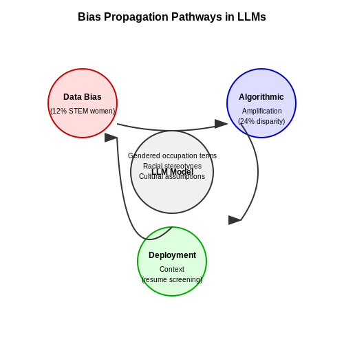
Bias in LLMs arises from three primary sources: data bias (unrepresentative or prejudiced training corpora), algorithmic bias (amplification of disparities during training), and deployment bias (contextual mismatches between training and real-world use). For instance, an LLM trained on historical texts may inherit gendered language patterns, as shown in the probability disparity for occupation-related terms:
Such disparities correlate with real-world demographic imbalances in profession gender ratios, but their amplification by models can entrench stereotypes.
Quantifying Harm: Disparate Impact Metrics
Disparate impact analysis measures bias through comparative performance across demographic groups. For binary classification tasks (e.g., resume screening), the ratio of positive outcomes between groups should ideally approximate 1.0. A common fairness metric is:
where G denotes group membership and Ŷ the model's prediction. Ratios below 0.8 typically indicate unlawful discrimination under U.S. EEOC guidelines.
Case Study: Gender Bias in Career Recommendations
In 2022, an audit of GPT-3 revealed that prompts containing female pronouns received STEM career suggestions 24% less frequently than male equivalents. The bias traced to underrepresentation of women in STEM-related training data (12-22% of mentions) and skewed co-occurrence statistics in web texts. Corrective measures required:
- Re-weighting training data to balance gender references
- Adversarial debiasing during fine-tuning
- Post-hoc output filtering using fairness classifiers
Legal and Regulatory Frameworks
The EU AI Act classifies high-risk LLM applications (e.g., hiring tools) as requiring mandatory bias assessments. In the U.S., the Algorithmic Accountability Act of 2023 mandates impact assessments for systems affecting protected classes. Technical compliance involves:
where ε is a tolerance threshold (typically 0.05) and G encompasses protected attributes like race or disability status.
Mitigation Trade-offs
Bias mitigation often involves accuracy-fairness trade-offs quantified by Pareto frontiers. For a model with original accuracy A₀ and bias metric B₀, debiasing may yield:
Empirical studies show ∆A/∆B ratios of 0.3-0.8 for common techniques like reweighting versus 0.1-0.3 for adversarial methods, highlighting the need for context-aware mitigation strategies.
6.2 Current Regulatory Landscape
The regulatory landscape for bias and fairness in large language models (LLMs) is rapidly evolving, with governments, international organizations, and industry consortia establishing frameworks to mitigate risks. The European Union’s Artificial Intelligence Act (AIA) categorizes high-risk AI systems, including those used in recruitment, education, and law enforcement, mandating transparency, bias audits, and human oversight. Non-compliance can result in fines up to 6% of global revenue, reflecting the EU’s stringent approach to algorithmic accountability.
In the United States, the Algorithmic Accountability Act and NIST AI Risk Management Framework emphasize post-deployment audits and impact assessments. The Federal Trade Commission (FTC) has also intervened under Section 5 of the FTC Act, penalizing companies for biased AI outcomes. For instance, in 2023, the FTC required an LLM developer to delete improperly collected data and implement fairness checks after discriminatory hiring recommendations.
Key Regulatory Instruments
- ISO/IEC 42001: The first international standard for AI management systems, requiring fairness metrics like demographic parity and equalized odds.
- OECD AI Principles: Advocate for proactive bias testing across the AI lifecycle, endorsed by 46 countries.
- Singapore’s IMDA Model AI Governance Framework: Recommends disaggregated performance metrics by gender, ethnicity, and age.
Mathematical Compliance Criteria
Regulators often require statistical fairness metrics. For example, the AIA references disparate impact ratio:
where Z denotes protected attributes, and Ŷ is the model’s prediction. A ratio below 0.8 or above 1.25 may trigger regulatory scrutiny.
Enforcement Mechanisms
Authorities employ:
- Third-party audits: Certified bodies assess models using standardized datasets (e.g., BiasBench for LLMs).
- Adversarial testing: Red-teaming exercises to uncover hidden biases, now mandated by the U.S. Executive Order 14110.
- Public disclosure: The EU Digital Services Act requires LLM providers to publish bias mitigation strategies and audit results.
Jurisdictional Challenges
Divergent standards create compliance complexities. China’s Generative AI Service Management Measures prioritize ideological alignment over demographic fairness, while Canada’s AIDA focuses on harm prevention. Multinational LLM deployments must reconcile these through:
- Modular fairness pipelines that adapt to regional laws.
- Differential privacy techniques to satisfy conflicting data protection rules (e.g., GDPR vs. China’s DSL).
6.3 Best Practices for Compliance and Transparency
Documentation and Model Cards
Comprehensive documentation is critical for ensuring transparency in LLMs. Model cards should include detailed metadata such as training data sources, demographic distributions, and potential biases. The Model Card Toolkit by Google provides a standardized framework for documenting model behavior, intended use cases, and limitations. For example, documenting that a model was trained on predominantly English-language data from North America helps users understand potential geographic biases.
Bias Mitigation Techniques
Several algorithmic approaches can reduce bias in LLMs:
- Reweighting: Adjusting sample weights during training to balance underrepresented groups.
- Adversarial Debiasing: Using adversarial networks to minimize correlation between protected attributes (e.g., gender, race) and model predictions.
- Fairness Constraints: Incorporating fairness metrics like demographic parity or equalized odds directly into the optimization objective.
Continuous Monitoring and Auditing
Bias detection should not be a one-time activity. Implement automated pipelines that:
- Track model performance across demographic subgroups over time
- Flag statistically significant drifts in fairness metrics
- Trigger alerts when bias thresholds are violated
Stakeholder Engagement
Effective compliance requires collaboration with domain experts from affected communities. Establish:
- External review boards with diverse representation
- Public comment periods for high-impact models
- Transparency reports detailing audit findings and mitigation efforts
Regulatory Alignment
Align audit processes with emerging frameworks like:
- EU AI Act's risk-based classification
- NIST AI Risk Management Framework
- OECD AI Principles
Technical Implementation
Open-source tools facilitate compliance:
from fairness_metrics import DemographicParity
from model_audit import BiasAuditor

auditor = BiasAuditor(
    model=llm_pipeline,
    metrics=[DemographicParity()],
    protected_attributes=['gender', 'race']
)
report = auditor.generate_report(test_data)
7. Key Research Papers and Articles
7.1 Key Research Papers and Articles
- Policy advice and best practices on bias and fairness in AI — The literature addressing bias and fairness in AI models (fair-AI) is growing at a fast pace, making it difficult for novel researchers and practitioners to have a bird's-eye view picture of the field. In particular, many policy initiatives, standards, and best practices in fair-AI have been proposed for setting principles, procedures, and knowledge bases to guide and operationalize the ...
- AI Fairness in Data Management and Analytics: A Review on ... - MDPI — This article provides a comprehensive overview of the fairness issues in artificial intelligence (AI) systems, delving into its background, definition, and development process. The article explores the fairness problem in AI through practical applications and current advances and focuses on bias analysis and fairness training as key research directions. The paper explains in detail the concept ...
- Fairness and Bias in Artificial Intelligence: A Brief Survey of ... - MDPI — The significant advancements in applying artificial intelligence (AI) to healthcare decision-making, medical diagnosis, and other domains have simultaneously raised concerns about the fairness and bias of AI systems. This is particularly critical in areas like healthcare, employment, criminal justice, credit scoring, and increasingly, in generative AI models (GenAI) that produce synthetic media.
- A Survey on Fairness in Large Language Models - arXiv.org — In this paper, we provide a comprehensive review of related research on fairness in LLMs, where the overall architecture is shown in Figure 1.According to the magnitude of the parameter and the training paradigm, we classify the fairness studies of LLMs into two categories: the studies of medium-sized LLMs under the fine-tuning paradigm and the studies of large-sized LLMs under the prompting ...
- Auditing the AI auditors: A framework for evaluating fairness and bias ... — Researchers, governments, ethics watchdogs, and the public are increasingly voicing concerns about unfairness and bias in artificial intelligence (AI)-based decision tools. Psychology's more-than-a-century of research on the measurement of psychological traits and the prediction of human behavior can benefit such conversations, yet psychological researchers often find themselves excluded due ...
- Unmasking bias in artificial intelligence: a systematic review of bias ... — The review identified key biases, outlined strategies for detecting and mitigating bias throughout the AI model development, and analyzed metrics for bias assessment. Results Of the 450 articles retrieved, 20 met our criteria, revealing 6 major bias types: algorithmic, confounding, implicit, measurement, selection, and temporal.
- (PDF) Bias Detection and Fairness in Large Language Models for ... — Bias Detection and Fairness in Large Language Models for Financial Services March 2025 International Journal of Scientific Research in Computer Science Engineering and Information Technology 11(2 ...
- Full article: AI Ethics: Integrating Transparency, Fairness, and ... — Post-hoc fairness auditing tools, such as AI Fairness 360 (AIF360), provide an open-source toolkit that measures and mitigates bias in deployed models. These tools can be integrated into AI governance processes, ensuring that models remain fair and unbiased as they encounter new data in real-world environments.
- Considerations in the reliability and fairness audits of predictive ... — However, there is a gap of operational guidance for performing reliability and fairness audits in practice. Following guideline recommendations, we conducted a reliability audit of two models based on model performance and calibration as well as a fairness audit based on summary statistics, subgroup performance and subgroup calibration.
- A Comprehensive Survey of Bias in LLMs: Current ... - ResearchGate — in bias research is the lack of transparency in the training processes and model architectures of LLMs, making it difficult to trace the origin of biases. Current models are often "black boxes,"
7.2 Recommended Books and Reports
- Addressing Bias and Fairness in Machine Learning: A Practical Guide and ... — This tutorial aims to bridge the gap between research and practice, providing an in-depth exploration of algorithmic fairness, encompassing metrics and definitions, practical case studies, data bias understanding, bias mitigation and model fairness audits using the Aequitas toolkit.
- [1811.05577] Aequitas: A Bias and Fairness Audit Toolkit - ar5iv — We present Aequitas, an open source bias and fairness audit toolkit that was released in 2018 and it is an intuitive and easy to use addition to the machine learning workflow, enabling users to seamlessly test models for several bias and fairness metrics in relation to multiple population sub-groups.
- Aequitas: A Bias and Fairness Audit Toolkit — We present Aequitas, an open source bias and fairness audit toolkit that was released in 2018 and it is an intuitive and easy to use addition to the machine learning work ow, enabling users to seamlessly test models for several bias and fairness metrics in relation to multiple population sub-groups.
- Fairness Score and process standardization: framework for fairness ... — Our proposal is different as we focus on the practical implementation aspects aiming to standardize the audit procedure to check the fairness of an AI system to enhance its trustworthiness. While most researchers have proposed different metrics to check for biases, we consider these metrics and present an integrated Fairness Score and Bias Index.
- Multifaceted Assessment of Responsible Use and Bias in Language Models ... — Echterhoff et al. [21] designed a framework to uncover, evaluate, and mitigate cognitive biases in LLMs. The Stanford Holistic Evaluation of Language Models (HELM) [22] offers a comprehensive approach for evaluating LLMs across a broad spectrum of metrics beyond mere accuracy to include fairness, bias, and toxicity.
- Auditing the AI auditors: A framework for evaluating fairness and bias ... — Landers and Behrend [52] introduce a framework for evaluating fairness and bias in high-stakes AI predictive models for decisionmaking from a psychological perspective.
- PDF On Bias and Fairness in LMs - Fatma Elsafoury — [5] On the Intrinsic and Extrinsic Fairness Evaluation Metrics for Contextual Language [6] Bias in Representations. Bios: A Case Study of Semantic Representation bias in High-Stakes [7] Your Settings.
- (PDF) Bias Detection and Fairness in Large Language Models for ... — This article addresses the critical issue of algorithmic bias and fairness in Large Language Models (LLMs) deployed across financial services. As these powerful AI systems increasingly influence ...
- Bias and Fairness | SpringerLink — Fairness Audits: Fairness audits involve a comprehensive review of data collection, preprocessing, and model development processes to identify potential sources of bias.
- Challenging Fairness: A Comprehensive Exploration of Bias in LLM-Based ... — This study investigates the intricate relationship between bias and LLM-based recommendation sys-tems, with a focus on music, song, and book recommendations across diverse demographic and cultural groups. Through a com-prehensive analysis conducted over different LLM-models, this paper evaluates the impact of bias on recommendation outcomes.
7.3 Online Resources and Communities
- LLMs and Ethics: Bias, Fairness, and Transparency - Medium — 7. LLMs and Ethics: Bias, Fairness, and Transparency: — Blog 7/10 (LLMs and Ethics: Bias, Fairness, and Transparency) — Abstract: Understand the critical concerns surrounding LLMs. Delve into the intrinsic biases present, the need for fairness in outputs, and the ongoing research and practices to make these models transparent and ethical. 8.
- Chapter 11 Bias and Fairness | Big Data and Social Science — 11.7 Aequitas - A Toolkit for Auditing Bias and Fairness in Machine Learning Models. To help data scientists and policymakers make informed decisions about bias and fairness in their applications, we developed Aequitas, an open source 97 bias and fairness audit toolkit that was released in May 2018 98. It is an intuitive and easy to use ...
- Bias in LLMs: Mitigating Discrimination or Reinforcing It? — Bias in large language models (LLMs) has several sources: 1. Data Imbalance: The training datasets might not accurately reflect some demographic groups, making the model inclined to prefer overrepresented groups in its predictions and outputs. 2. Stereotypes in Training Data: The occurrence of deep-rooted stereotypes and prejudices within texts used for training LLMs will make these models ...
- Bias and Fairness in Large Language Models: A Survey — Abstract. Rapid advancements of large language models (LLMs) have enabled the processing, understanding, and generation of human-like text, with increasing integration into systems that touch our social sphere. Despite this success, these models can learn, perpetuate, and amplify harmful social biases. In this article, we present a comprehensive survey of bias evaluation and mitigation ...
- Biases and Fairness in LLMs - SpringerLink — Table 10.1 has covered 12 survey sources as a general survey papers and blog survey, out of these, 6 papers have explored with the research survey papers to highlight the bias and fairness in large language models; 5 papers explored the existing blog survey to present the literature of bias and fairness in large language models and one paper ...
- [1811.05577] Aequitas: A Bias and Fairness Audit Toolkit - arXiv.org — Recent work has raised concerns on the risk of unintended bias in AI systems being used nowadays that can affect individuals unfairly based on race, gender or religion, among other possible characteristics. While a lot of bias metrics and fairness definitions have been proposed in recent years, there is no consensus on which metric/definition should be used and there are very few available ...
- An Open-source Project for Ethical Ai and Fairness Auditing: Building ... — It supports critical fairness metrics and auditing facilities, which make it suitable for organizations preferring relatively simple models or a less steep learning curve. 8.2 Fairness-Focused Libraries and Toolkits This project uses additional reasonably related libraries to enhance its bias detection and prevention and enable customers to ...
- (PDF) Bias Detection and Fairness in Large Language Models for ... — Bias Detection and Fairness in Large Language Models for Financial Services March 2025 International Journal of Scientific Research in Computer Science Engineering and Information Technology 11(2 ...
- PDF On Bias and Fairness in LMs - Fatma Elsafoury — Language Representations.[6] Bias in Bios: A Case Study of Semantic Representation bias in High-[7] Your Fairness May Vary: Pre-trained Language Model Fairness in Toxic Stakes Settings. Classification.[8] Nuanced Metrics for Measuring Unintended Bias with Real Data For Text Classification .
- (PDF) Ethical Considerations and Bias Mitigation in Large Language ... — Bias in LLMs also raises concerns about fairness and justice. When AI systems make decisions that affect people's lives—such as in hiring, law enforcement, or lending—the ethical expectation