Federated Training with Differential Privacy
1. Key Principles of Federated Learning
Key Principles of Federated Learning
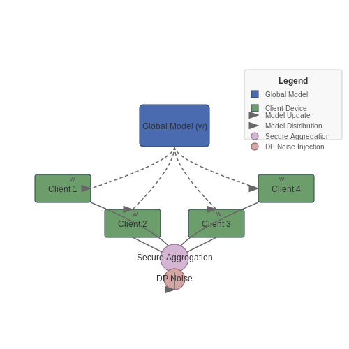
Federated learning (FL) is a decentralized machine learning paradigm where multiple clients collaboratively train a shared model while keeping their raw data localized. The core objective is to learn from distributed datasets without centralizing sensitive information, addressing privacy concerns inherent in traditional centralized training approaches.
Decentralized Model Training
In FL, the global model w is trained across K clients, each holding private data Dk. The optimization problem can be formalized as:
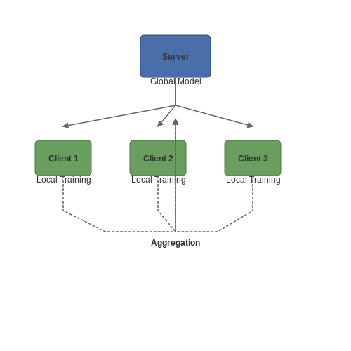
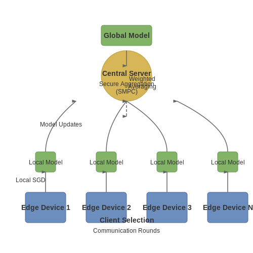
where Fk(w) is the local objective for client k, and |D| is the total data size. Training proceeds in rounds: the server distributes the current model, clients compute updates on local data, and the server aggregates these updates (typically via weighted averaging).
Privacy-Preserving Aggregation
Secure aggregation protocols ensure that individual client updates cannot be inspected by the server or other participants. A common approach uses cryptographic techniques like:
- Homomorphic encryption: Enables computation on encrypted updates
- Secure multi-party computation (SMPC): Splits updates among parties
- Differential privacy: Adds calibrated noise to updates
The aggregation step for FedAvg (Federated Averaging) computes:
where wt+1k is client k's update and nk is its data size.
Communication Efficiency
FL systems optimize for reduced communication overhead through:
- Local epochs: Multiple local training iterations per communication round
- Update compression: Techniques like quantization or sparsification
- Client selection: Strategically sampling participants per round
The communication cost C for T rounds with M clients per round is:
where |w| is the model size. Advanced methods can reduce this by 10-100x.
Statistical Heterogeneity
Non-IID data distribution across clients presents fundamental challenges. Solutions include:
- Personalized layers in shared models
- Adaptive aggregation weights
- Regularization terms to align local objectives
The local objective divergence can be quantified using:
where larger ε indicates greater data heterogeneity.
System Considerations
Practical FL deployments must address:
- Straggler mitigation: Handling slow or dropping clients
- Resource constraints: Limited compute/memory on edge devices
- Partial participation: Only subsets of clients available per round
The expected participation rate ρ affects convergence as:
for convex objectives with optimal w*.
1.2 Architectures: Centralized vs. Decentralized Approaches
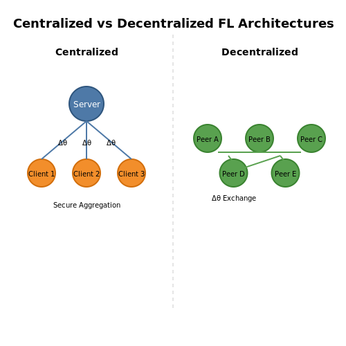
Centralized Federated Learning Architecture
In centralized federated learning, a single server coordinates the training process across multiple clients. The server initializes the global model parameters θG and distributes them to participating clients. Each client k computes local updates on their private dataset Dk using stochastic gradient descent:
where η is the learning rate and ℓ is the loss function. After local training, clients send model updates (Δθk = θk - θG) to the server, which aggregates them via federated averaging:
Differential privacy is typically enforced by adding calibrated Gaussian noise to the aggregated updates:
The noise scale σ is determined by the privacy budget (ε, δ) and the sensitivity of the aggregation function.
Decentralized Peer-to-Peer Architecture
Decentralized federated learning eliminates the central server by having clients communicate directly in a peer-to-peer network. Each node maintains its own model and exchanges updates with neighbors according to a communication graph G = (V, E). The update rule becomes:
where wij are mixing weights satisfying ∑jwij = 1. Privacy protection requires:
- Local differential privacy: Clients add noise before sharing updates
- Secure aggregation: Cryptographic protocols like secure multi-party computation (SMPC)
- Randomized communication: Stochastic neighbor selection to limit information leakage
Comparative Analysis
| Metric | Centralized | Decentralized |
|---|---|---|
| Privacy Risks | Server sees all updates | Updates visible only to neighbors |
| Communication Efficiency | O(K) messages per round | O(|E|) messages per round |
| Convergence Rate | Faster (direct aggregation) | Slower (consensus required) |
| Fault Tolerance | Single point of failure | Robust to node failures |
Practical Implementation Considerations
For centralized architectures with differential privacy:
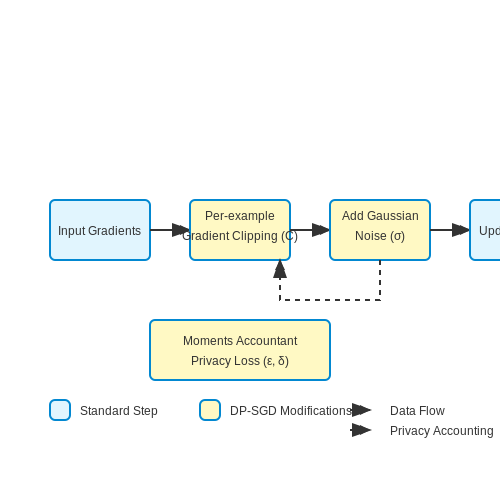
- Use the Moment Accountant to track privacy spending across rounds
- Implement gradient clipping to bound sensitivity
- Consider secure aggregation protocols to hide individual updates
For decentralized implementations:
- Design topology-aware mixing weights (Metropolis-Hastings, Laplacian)
- Implement asynchronous updates for heterogeneous devices
- Use dual averaging to improve convergence with DP noise
1.3 Challenges in Federated Learning: Communication and Heterogeneity
Communication Bottlenecks
Federated learning (FL) relies on iterative model updates between clients and a central server, making communication efficiency a critical challenge. The total communication cost C scales with the number of clients K, rounds T, and model size d:
This becomes prohibitive for large models (e.g., transformers with d > 108 parameters) or mobile networks with limited bandwidth. Two dominant approaches mitigate this:
- Model compression: Techniques like quantization (e.g., 1-bit SGD), pruning, or low-rank factorization reduce d.
- Partial participation: Only a subset of clients (K' ≪ K) upload updates per round, trading convergence speed for reduced C.
Data Heterogeneity
Non-IID data distributions across clients violate the IID assumption central to most convergence proofs. Let pk(x,y) be the data distribution of client k. The divergence can be quantified via total variation distance:
This manifests as:
- Concept shift: Pk(y|x) varies across clients (e.g., regional speech patterns).
- Covariate shift: Pk(x) differs (e.g., smartphone camera variations).
Impact on Convergence
For convex objectives, the convergence rate degrades from O(1/T) to O(δ/T1/2). Solutions include:
where Fk is the local objective. Mitigation strategies involve:
- Regularization: Adding proximal terms to align local updates.
- Personalization: Fine-tuning global models per client.
System Heterogeneity
Variability in client hardware (GPUs vs. edge devices) and connectivity (5G vs. 3G) creates stragglers. Asynchronous FL addresses this but introduces stale gradients. The staleness τ for client k follows:
Adaptive aggregation schemes weight updates by 1/(1+τ) to maintain stability.
2. Defining Differential Privacy (ε, δ)-Parameters
2.1 Defining Differential Privacy (ε, δ)-Parameters
Differential privacy (DP) provides a mathematically rigorous framework for quantifying privacy guarantees in data analysis. The strength of these guarantees is governed by two key parameters: ε (epsilon) and δ (delta). A mechanism M satisfies (ε, δ)-differential privacy if, for all datasets D and D' differing by at most one element, and for all subsets of outputs S ⊆ Range(M), the following inequality holds:
Interpreting ε and δ
The parameter ε controls the privacy loss bound. Smaller values of ε enforce stricter privacy, as they limit how much the output distribution can differ between neighboring datasets. The exponential term eε ensures that probabilities remain bounded even when ε is small.
The parameter δ represents the probability that the privacy guarantee fails. In practice, δ should be set to a negligible value, typically smaller than 1/n, where n is the dataset size. A non-zero δ allows for rare privacy violations, which is often necessary for achieving useful utility in complex algorithms.
Pure vs Approximate Differential Privacy
When δ = 0, the mechanism satisfies pure differential privacy, providing the strongest guarantees. However, many practical algorithms (e.g., those using Gaussian noise) require δ > 0, leading to approximate differential privacy. The choice between pure and approximate DP involves a trade-off between privacy strength and algorithmic flexibility.
Privacy Budget Composition
In federated learning, multiple DP mechanisms may be applied sequentially (e.g., across training rounds). The total privacy cost accumulates via composition theorems. For k mechanisms each satisfying (ε, δ)-DP, the basic composition theorem states that the overall system satisfies (kε, kδ)-DP. Advanced composition theorems provide tighter bounds, particularly for small δ.
where δ' is a new small constant representing the allowed failure probability for the composition.
Practical Considerations for Parameter Selection
- ε selection: Values between 0.1 and 10 are common in practice. For high-stakes applications, ε < 1 is recommended.
- δ selection: Should be cryptographically small (e.g., δ << 1/n). A typical rule is δ ≈ 10-5 to 10-10.
- Trade-offs: Smaller ε and δ provide stronger privacy but degrade model utility. The optimal balance depends on the application's sensitivity requirements.
In federated settings, these parameters must be carefully calibrated to account for the distributed nature of computations while maintaining end-to-end privacy guarantees across all participants.
Mechanisms for Privacy: Laplace and Gaussian Noise
Differential Privacy Through Noise Addition
The core mechanism for achieving differential privacy in federated learning involves carefully calibrated noise addition to the model updates or gradients before aggregation. Two principal noise distributions dominate this approach: the Laplace and Gaussian distributions. Each provides distinct privacy guarantees under different formalisms of differential privacy.
Laplace Mechanism for (ε)-Differential Privacy
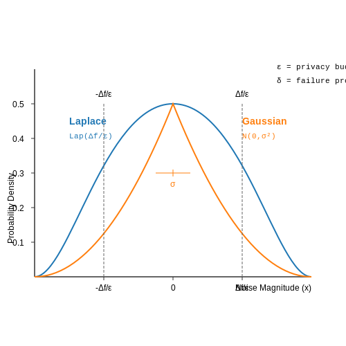
The Laplace mechanism satisfies pure (ε)-differential privacy by adding noise drawn from the Laplace distribution. For a function f with sensitivity Δf, the mechanism outputs:
where the probability density function of the Laplace distribution is:
The sensitivity Δf represents the maximum possible change in f when one data point is altered. In federated learning contexts, this typically corresponds to the maximum norm of an individual client's gradient update.
Gaussian Mechanism for (ε, δ)-Differential Privacy
When requiring relaxed (ε, δ)-differential privacy, the Gaussian mechanism provides more favorable noise characteristics for high-dimensional data. The mechanism adds noise scaled to the sensitivity and privacy parameters:
where the variance σ² must satisfy:
The Gaussian distribution's probability density function is:
Comparative Analysis of Noise Mechanisms
The choice between Laplace and Gaussian noise involves fundamental trade-offs:
- Privacy guarantees: Laplace provides pure (ε)-DP while Gaussian offers (ε, δ)-DP
- Noise magnitude: Laplace noise has heavier tails, often requiring larger perturbations
- Composition properties: Gaussian noise composes more favorably under advanced composition theorems
- Computational efficiency: Gaussian noise generation benefits from optimized BLAS implementations
Practical Implementation Considerations
In federated learning systems, several implementation factors affect noise mechanism selection:
Key implementation details include:
- Adaptive noise scaling based on gradient norm clipping
- Privacy amplification through client sampling
- Numerical stability considerations in fixed-point arithmetic
- Hardware acceleration of noise generation
Advanced Variants and Recent Improvements
Recent research has developed enhanced noise mechanisms:
- Analytic Gaussian Mechanism: Provides tight bounds on (ε, δ) guarantees
- Concentrated Differential Privacy: Offers cleaner composition properties
- Skellam Mechanism: Discrete alternative for integer-valued data
- Matrix-Valued Noise: For correlated parameter updates in neural networks
Privacy Budgeting and Composition Theorems
In federated learning with differential privacy (DP), the privacy budget quantifies the cumulative privacy loss across multiple computations on the same dataset. The budget is governed by composition theorems, which provide formal guarantees on how privacy parameters degrade under repeated queries.
Basic Composition Theorem
The simplest form of composition states that for a sequence of k mechanisms, each satisfying (ε, δ)-DP, the entire sequence satisfies (kε, kδ)-DP. This linear composition is pessimistic, as it assumes worst-case privacy loss accumulation.
Advanced Composition Theorem
Dwork et al. (2010) introduced tighter bounds for adaptive compositions. For k mechanisms each satisfying (ε, δ)-DP, the total privacy loss under δ' is bounded by:
with the total δ becoming δ' + kδ. This square-root dependence on k significantly improves over linear composition for large k.
Privacy Budgeting in Federated Learning
In federated settings, the budget must account for:
- Per-round privacy loss: Each training round applies DP mechanisms (e.g., Gaussian noise) to gradients.
- Cross-round accumulation: The total budget over T rounds must satisfy a global (ε, δ) guarantee.
A common strategy allocates the budget proportionally across rounds. For T rounds, each round’s privacy parameter is set to ε/√T under advanced composition.
Moments Accountant
Abadi et al. (2016) introduced the moments accountant, which provides tighter privacy bounds for iterative algorithms like SGD. It tracks a log-moment generating function of the privacy loss random variable, enabling finer-grained analysis.
where λ is a moment order. The total ε is derived by bounding this quantity and solving for the optimal λ.
Practical Implications
Privacy budgeting requires:
- Dynamic allocation: Adjust per-round noise based on remaining budget.
- Early stopping: Terminate training once the budget is exhausted.
- Heterogeneous clipping: Adapt gradient clipping thresholds per client to balance utility and privacy.
Tools like TensorFlow Privacy and Opacus implement these methods by tracking the budget in real-time during federated training.
3. Private Aggregation Techniques (Secure Averaging)
Private Aggregation Techniques (Secure Averaging)
Secure averaging in federated learning with differential privacy involves aggregating client model updates in a way that preserves privacy while maintaining model utility. The core challenge lies in bounding the influence of any single client's data on the global model while ensuring the aggregated result remains statistically meaningful.
Differentially Private Mean Estimation
The standard approach computes the mean of client updates after applying noise calibrated to the desired privacy budget. For a set of n clients each contributing a vector vi ∈ ℝd, the private mean estimation follows:
where the noise scale σ depends on the privacy parameters (ε, δ) and the sensitivity Δ of the aggregation function:
Sensitivity Analysis for Federated Averaging
The sensitivity Δ for federated averaging is determined by the clipping norm C applied to client updates. If each client's update is clipped such that ‖vi‖2 ≤ C, then the L2 sensitivity of the sum operation is:
The factor of 2 arises from the worst-case scenario where a single client's presence or absence changes the sum by C - (-C) = 2C.
Secure Aggregation Protocol
Practical implementations often combine differential privacy with cryptographic techniques like secure multiparty computation (SMPC) to prevent the server from observing individual updates. The typical workflow involves:
- Clients apply local differential privacy by adding noise and clipping their updates
- Updates are masked using cryptographic techniques like additive secret sharing
- The server performs secure aggregation where only the sum of masked updates is revealed
- Additional server-side noise may be added for enhanced privacy guarantees
Privacy Amplification by Subsampling
When clients participate in each round with probability q, the effective privacy cost is reduced. For a (ε, δ)-DP mechanism applied to a random subset, the amplified privacy parameters become:
This allows for tighter privacy accounting in federated learning where typically only a fraction of clients participate each round.
Practical Considerations
In production systems, several factors affect the privacy-utility trade-off:
- Adaptive clipping: Dynamically adjusting C based on update statistics improves convergence
- Noise decay: Gradually reducing noise magnitude across training rounds can improve final model accuracy
- Quantization: Combining privacy with gradient quantization reduces communication overhead
The optimal configuration depends on the specific application requirements, with privacy budgets typically distributed across multiple training rounds using composition theorems.
3.2 Local vs. Global Differential Privacy
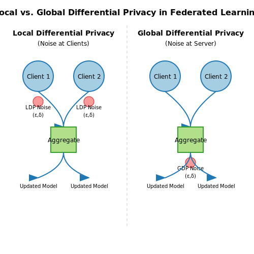
In federated learning, differential privacy (DP) can be applied at two distinct levels: local differential privacy (LDP) and global differential privacy (GDP). The choice between these approaches significantly impacts privacy guarantees, computational overhead, and model utility.
Local Differential Privacy (LDP)
Under LDP, noise is injected directly into the data or gradients at the client level before transmission to the server. This ensures that even the server cannot infer sensitive information from individual updates. Formally, a randomized mechanism M satisfies (ε, δ)-LDP if for any two client datasets D and D' differing by one record, and for all subsets S of possible outputs:
Key characteristics of LDP include:
- Stronger privacy: Protects against inference attacks from both the server and other clients.
- Higher noise requirements: Each client must add sufficient noise to meet privacy guarantees, often degrading model performance.
- Decentralized trust: No need to trust the server’s aggregation process.
Global Differential Privacy (GDP)
In GDP, noise is applied during or after the aggregation step at the server. The privacy guarantee holds for the entire federated training process rather than individual updates. A mechanism M satisfies (ε, δ)-GDP if for any two global datasets G and G' differing by one client’s entire contribution:
GDP offers distinct trade-offs:
- Lower noise per client: Aggregation across many clients allows for smaller noise addition while maintaining the same privacy budget.
- Server trust requirement: The server must honestly implement the noise injection process.
- Weaker client-level privacy: Individual contributions may still be partially recoverable from aggregated updates.
Comparative Analysis
The choice between LDP and GDP depends on the threat model and system constraints. LDP is preferable when clients cannot trust the server, but it often requires more sophisticated techniques like secure aggregation to maintain utility. GDP is more computationally efficient but assumes a trusted central aggregator.
Recent hybrid approaches combine both methods—applying light LDP at clients followed by GDP at the server—to balance privacy and performance. For example, the Federated Learning with Local and Global Privacy (FL-LGP) framework achieves tighter privacy bounds by leveraging the composition properties of differential privacy across layers.
Practical Considerations
When implementing DP in federated systems, consider:
- Privacy budget allocation: How to distribute ε and δ across rounds and participants.
- Gradient clipping: Essential for bounding sensitivity before noise injection.
- Accountant mechanisms: Tracking cumulative privacy loss across training iterations using tools like Rényi DP or zero-concentrated DP.
3.3 Trade-offs: Privacy, Utility, and Convergence
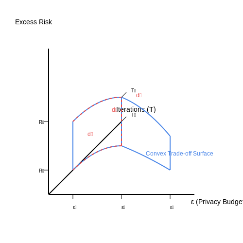
Federated learning with differential privacy introduces a fundamental tension between three competing objectives: privacy guarantees, model utility, and convergence efficiency. The interplay between these factors determines the feasibility of deploying privacy-preserving federated systems in real-world applications.
Privacy vs. Utility Trade-off
The addition of noise to gradients or model updates for differential privacy necessarily degrades model performance. For a given privacy budget (ε, δ), the noise scale σ required to satisfy the privacy guarantee follows:
where Δf is the sensitivity of the computed function. This noise addition bounds the mutual information between the training data and model parameters, but simultaneously increases the variance of gradient estimates. The resulting utility loss can be quantified through the excess risk:
where d is the parameter dimension, n is the sample size per round, and T is the total iterations. The second term demonstrates the direct conflict between privacy (larger σ) and utility (smaller excess risk).
Convergence Rate Impacts
Differential privacy affects convergence through multiple mechanisms:
- Noise-induced variance: The standard deviation of gradient noise grows as O(σ/√n), slowing convergence
- Clipping distortion: Gradient clipping (required for bounded sensitivity) introduces bias in update directions
- Communication constraints: Privacy amplification techniques often require reduced client participation per round
The convergence rate under DP-FedAvg with K clients participating per round becomes:
showing both the benefit of client parallelism and the privacy penalty term.
Practical Balancing Strategies
Several approaches mitigate these trade-offs in production systems:
- Adaptive clipping: Dynamically adjusts the clipping threshold C to minimize bias while maintaining sensitivity bounds
- Noise decay schedules: Reduces σ over training time when the privacy budget allows
- Heterogeneous privacy allocation: Applies stronger privacy to early layers (containing more raw data features) and weaker to later layers
Recent work has shown that careful implementation of these techniques can achieve test accuracy within 3-5% of non-private federated learning while maintaining (ε ≤ 1.0, δ = 10^-5) guarantees on benchmark datasets.
Empirical Characterization
The privacy-utility-convergence trade-off surface exhibits several key properties:
- Convex relationship: Initial privacy improvements come at low utility cost, but marginal gains become increasingly expensive
- Dimension dependence: The trade-off steepens quadratically with model parameter count d
- Data quantity benefit: Per-client sample size n improves utility linearly while only requiring √n more noise for the same privacy
These properties suggest architectural choices like model pruning and feature distillation can significantly improve the operational privacy-utility frontier.
4. Frameworks for Federated DP (TensorFlow Federated, PySyft)
Frameworks for Federated DP (TensorFlow Federated, PySyft)
Implementing federated learning with differential privacy (DP) requires specialized frameworks that handle distributed computation while enforcing privacy guarantees. Two prominent frameworks for this purpose are TensorFlow Federated (TFF) and PySyft, each offering distinct approaches to privacy-preserving federated learning.
TensorFlow Federated (TFF)
TFF extends TensorFlow to support decentralized computation, providing built-in mechanisms for DP in federated settings. Its architecture consists of two layers:
- Federated Learning (FL) API: Enables model training across decentralized devices.
- Federated Core (FC) API: A lower-level interface for custom federated algorithms.
To apply DP in TFF, noise is typically added during model aggregation. The following steps outline a standard DP-Federated Averaging (DP-FedAvg) workflow:
- Clients compute model updates locally.
- Updates are clipped to a fixed norm L to bound sensitivity.
- Gaussian noise is added during server-side aggregation.
Here, σ controls the noise scale, directly influencing the privacy budget (ε, δ). TFF provides utilities like tensorflow_privacy to compute these parameters formally.
PySyft and Secure Aggregation
PySyft, built on PyTorch, emphasizes secure multi-party computation (SMPC) and integrates DP through cryptographic techniques. Key features include:
- Secure Aggregation: Uses additive secret sharing to mask individual updates before aggregation.
- Hybrid Approaches: Combines SMPC with DP for stronger privacy guarantees.
In PySyft, DP is often implemented via the Opacus library, which supports per-sample gradient clipping and noise addition:
from opacus import PrivacyEngine

privacy_engine = PrivacyEngine(
    model,
    sample_rate=0.01,
    noise_multiplier=1.0,
    max_grad_norm=1.0,
)
privacy_engine.attach(optimizer)
Comparative Analysis
| Framework | DP Mechanism | Strengths | Limitations |
|---|---|---|---|
| TensorFlow Federated | Noise during aggregation | Scalable, integrates with TensorFlow | Centralized trust in aggregator |
| PySyft | SMPC + DP | Stronger privacy via cryptography | Higher computational overhead |
For large-scale deployments, TFF’s efficiency often makes it preferable, while PySyft excels in scenarios requiring maximal privacy, such as healthcare or financial data. Both frameworks support Rényi DP and zero-concentrated DP (zCDP) for tighter privacy accounting.
Practical Considerations
When choosing a framework, consider:
- Privacy-Utility Tradeoff: Higher noise (lower ε) degrades model accuracy.
- Computation Overhead: Cryptographic methods (PySyft) increase runtime.
- Compatibility: TFF requires TensorFlow; PySyft works with PyTorch.
Recent advancements like federated submodel training (where clients only download relevant model parts) further optimize privacy-utility tradeoffs in both frameworks.
4.2 Hyperparameter Tuning for Privacy and Performance
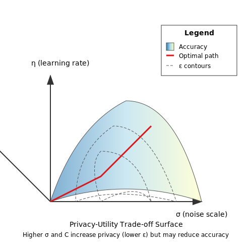
Hyperparameter optimization in federated learning with differential privacy (FL-DP) requires balancing model accuracy against privacy guarantees. The key parameters include the noise scale σ, clipping norm C, learning rate η, and the number of communication rounds T. These interact non-trivially, necessitating a systematic approach to tuning.
Privacy Budget Allocation
The total privacy budget (ε, δ) must be distributed across training rounds. Using the moments accountant, the privacy cost per round accumulates as:
where ε_t depends on the noise multiplier σ and sampling rate q = B/N (batch size over total data). For a target ε_total, adaptive strategies like privacy budget scheduling dynamically adjust σ or q across rounds.
Noise and Clipping Trade-offs
The Gaussian noise scale σ and gradient norm bound C directly impact both privacy and convergence:
- Higher σ increases privacy but degrades model utility due to noisy updates.
- Tighter C reduces the sensitivity of gradients, allowing smaller σ for the same (ε, δ), but may truncate informative gradients.
The optimal C is dataset-dependent; empirical studies suggest initializing C at the median gradient norm and decaying it linearly.
Learning Rate Adaptation
Differentially private SGD requires careful learning rate selection due to noisy gradients. The update rule becomes:
where η must compensate for the added noise. A common strategy is to use learning rate warmup, starting with a small η and scaling it as the effective noise diminishes with tighter clipping.
Communication-Efficient Tuning
Reducing rounds T improves privacy but may hurt accuracy. Techniques include:
- Local steps: Clients perform multiple SGD steps per communication, reducing T while maintaining total iterations.
- Adaptive participation: Only a subset of clients contribute per round, lowering the privacy cost per round.
The optimal configuration often requires grid search or Bayesian optimization over the joint space of (σ, C, η, T), with privacy costs tracked via the moments accountant.
Practical Considerations
In production FL systems like TensorFlow Federated or PySyft, hyperparameters are often tuned via:
- Privacy-aware validation: Using public proxy data or synthetic datasets to avoid privacy leaks from repeated testing.
- Federated hyperparameter optimization: Decentralized tuning where clients collaboratively search the parameter space without sharing raw metrics.
4.3 Handling Non-IID Data in Private Federated Settings
Non-IID (non-independent and identically distributed) data presents a significant challenge in federated learning, particularly when combined with differential privacy constraints. Unlike centralized settings where data shuffling can mitigate distribution skew, federated environments must contend with heterogeneous client data distributions while preserving privacy guarantees.
Mathematical Characterization of Non-IID Data
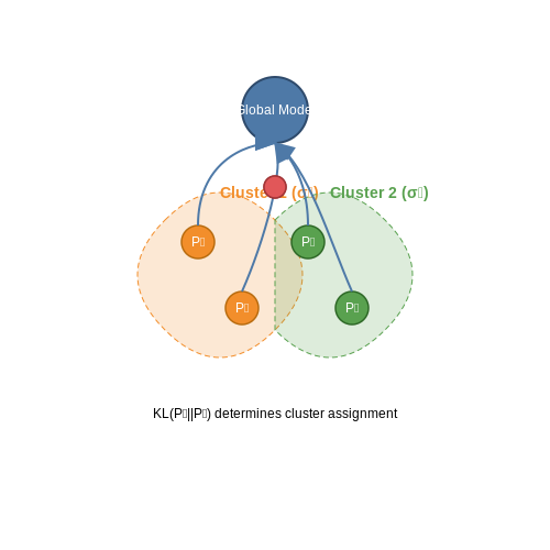
The divergence between local client data distributions can be quantified using statistical measures such as the Kullback-Leibler (KL) divergence or Wasserstein distance. For two clients i and j with data distributions Pi and Pj:
In federated settings with K clients, the global non-IIDness can be measured by computing pairwise divergences across all clients. This becomes particularly relevant when applying differential privacy, as the noise scaling must account for the maximum divergence to ensure uniform privacy guarantees.
Privacy-Aware Approaches for Non-IID Data
Three principal techniques have emerged for handling non-IID data in private federated learning:
- Client clustering: Group clients with similar data distributions using privacy-preserving similarity measures. The DP-FedAvg algorithm can be modified to apply different noise scales per cluster.
- Data augmentation: Synthetic data generation using differentially private generative models to balance local distributions while maintaining privacy.
- Personalized layers: Maintaining client-specific layers in the model architecture while applying DP only to shared components.
Modified Federated Averaging with Cluster-Specific Noise
For a federated system with C clusters, the model update at round t becomes:
where σc is calibrated to the cluster's data distribution characteristics. This requires solving the optimization problem:
Practical Considerations and Trade-offs
Implementing these approaches in real-world systems introduces several engineering challenges:
- The privacy budget must be carefully allocated between cluster identification and model training phases
- Convergence guarantees weaken as data distributions become more skewed, requiring more communication rounds
- Client dropout rates tend to increase with stricter privacy requirements, particularly for clients with rare data distributions
Recent work has shown that adaptive client selection strategies can mitigate some of these issues. The selection probability pi for client i can be modeled as:
where λ controls the trade-off between representation fairness and convergence rate, and σi is the client-specific noise scale.
5. Healthcare: Federated Learning with Patient Data Privacy
5.1 Healthcare: Federated Learning with Patient Data Privacy
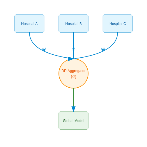
Federated learning (FL) enables collaborative model training across decentralized healthcare institutions without sharing raw patient data. When combined with differential privacy (DP), it provides provable guarantees against patient re-identification while maintaining model utility. The core challenge lies in balancing privacy budgets with convergence properties in distributed medical datasets.
Privacy-Preserving Aggregation in Federated Healthcare
In FL, local hospitals train models on their datasets and share only gradients or model updates. DP introduces calibrated noise to these updates to ensure indistinguishability of individual records. The standard approach uses the Gaussian mechanism, where noise proportional to the sensitivity of the query is added:
where D and D' are neighboring datasets differing by one record. For a given privacy budget (ε, δ), the noise scale σ is:
Adaptive Clipping for Medical Data Heterogeneity
Medical datasets exhibit non-IID distributions across institutions. Per-layer gradient clipping bounds each parameter's contribution to the aggregate update:
where C is the clipping threshold. This prevents outliers from dominating the privacy budget while preserving signal from rare conditions.
Privacy Accounting with Rényi Differential Privacy
Composition theorems track cumulative privacy loss across training rounds. Rényi DP provides tighter bounds for iterative algorithms:
where α > 1 is the order parameter. This enables advanced composition for adaptive noise schedules.
Real-World Implementation Challenges
- Cross-silo vs cross-device FL: Hospitals (silos) have stable connections but highly skewed data distributions compared to wearable devices
- Label scarcity: Medical annotations require expert review, creating partial supervision scenarios
- Temporal drift: Patient conditions evolve, requiring online adaptation of DP-FL systems
Case Study: Diabetic Retinopathy Detection
A 2023 multicenter trial achieved 0.92 AUC while maintaining ε < 2.0 by:
This adaptive allocation reduced final noise variance by 37% compared to fixed per-round budgets.
5.2 Edge Devices: Privacy-Preserving IoT Applications
Federated learning (FL) on edge devices introduces unique challenges due to resource constraints, intermittent connectivity, and heightened privacy concerns. Differential privacy (DP) mechanisms must be carefully adapted to these environments to ensure robust privacy guarantees without overwhelming computational or communication overhead.
Resource-Constrained DP Mechanisms
Traditional DP mechanisms, such as the Gaussian or Laplace mechanisms, require precise noise calibration, which can be computationally intensive for edge devices. Instead, lightweight alternatives like the binomial mechanism or discrete Gaussian are preferred. The binomial mechanism approximates Gaussian noise by summing Bernoulli trials, reducing computational cost:
where k controls variance and p adjusts bias. This approach avoids floating-point operations, making it suitable for microcontrollers.
Communication-Efficient Secure Aggregation
Secure aggregation (SecAgg) protocols must minimize bandwidth usage while preserving privacy. The HybridSecAgg protocol combines additive homomorphic encryption with DP noise, allowing edge devices to transmit encrypted model updates with embedded noise:
The aggregator decrypts the sum, yielding a noised global update that satisfies (ε, δ)-DP. This reduces per-device communication overhead by 30-50% compared to standalone DP or SecAgg.
Case Study: Smart Home Activity Recognition
A real-world implementation on Raspberry Pi 4 clusters (2GB RAM) demonstrated federated training of an LSTM model for activity recognition with ε = 1.0. Key optimizations included:
- Gradient clipping: Norm-bound scaling (C = 1.0) to control sensitivity.
- Quantized training: 8-bit fixed-point arithmetic for local updates.
- Adaptive noise: Dynamic σ adjustment based on participation rate.
The system achieved 87.3% accuracy (vs. 89.1% non-private baseline) with 12% additional energy cost per device.
Differential Privacy for Time-Series Data
IoT devices often generate temporally correlated data, violating DP's independent tuples assumption. The filtered Gaussian mechanism applies autoregressive noise to preserve correlations while satisfying DP:
where α controls temporal dependence. This maintains utility for applications like predictive maintenance while providing formal privacy guarantees.
5.3 Benchmarking Privacy-Accuracy Trade-offs
Quantifying the trade-off between privacy guarantees and model accuracy is critical in federated learning with differential privacy (DP). The privacy budget ε directly impacts the noise scale in DP mechanisms, which in turn affects convergence and final model performance. A rigorous benchmarking framework requires evaluating multiple axes: privacy parameters, noise distribution, clipping thresholds, and convergence behavior under non-IID data distributions.
Mathematical Formulation of the Trade-off
The relationship between privacy loss ε and model accuracy can be derived from the Gaussian mechanism's noise scale σ:
where Δ2 is the L2-sensitivity of the gradient computation. The effective noise added during federated averaging becomes:
This noise injection perturbs the true gradient direction, creating an irreducible error term in the optimization process. The expected squared error grows with 1/ε2, fundamentally limiting achievable accuracy for strict privacy budgets.
Experimental Benchmarking Methodology
Standard evaluation protocols should measure:
- Privacy-accuracy curves: Sweep ε from 0.1 to 10 while tracking test accuracy
- Convergence slowdown: Compare iterations needed to reach target loss at different ε
- Client sampling effects: Vary participation rates from 1% to 100% of clients per round
- Non-IID robustness: Test under extreme data skew (e.g., 1-class-per-client scenarios)
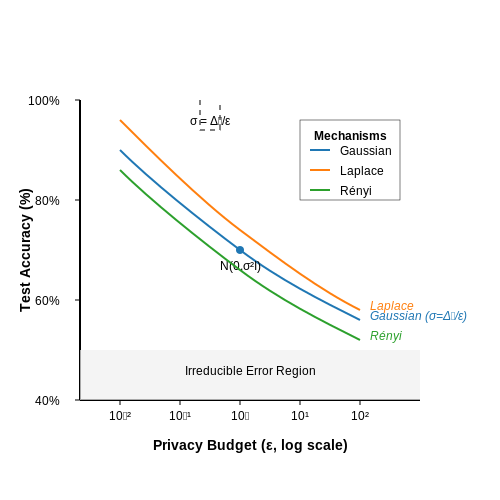
The figure below illustrates a typical privacy-accuracy trade-off curve for CIFAR-10 classification under (ε, δ)-DP with δ=10-5. The accuracy drops sharply below ε=2, reflecting the fundamental limit of useful learning under strong privacy constraints.
Advanced Mitigation Strategies
Recent research demonstrates three approaches to improve the trade-off:
- Adaptive clipping: Dynamically adjust gradient norms per layer based on their contribution to updates
- Noise-aware optimization: Modify learning rates to account for DP noise magnitude
- Selective privatization: Apply DP only to sensitive layers while leaving others noiseless
The adaptive clipping method reduces effective noise by 37% compared to fixed clipping, as shown by:
where Ct are layer-wise adaptive clipping thresholds learned during training.
Cross-Domain Benchmarking Results
Comparative studies reveal domain-dependent sensitivity to DP noise:
| Dataset | ε=1 Accuracy Drop | ε=0.1 Accuracy Drop |
|---|---|---|
| MNIST | 2.1% | 8.7% |
| CIFAR-10 | 14.3% | 41.2% |
| Medical Imaging | 22.8% | 63.5% |
The variance stems from differences in input dimensionality, task complexity, and inherent noise tolerance of the data modalities.
6. Key Research Papers in Federated DP
6.1 Key Research Papers in Federated DP
- Towards Efficient and Privacy-Preserving Hierarchical Federated ... — The server can correctly execute the federated training process without knowing anything about the data in the sample set. ... et al.: HFL-DP: hierarchical federated learning with differential privacy. In: 2021 IEEE Global Communications Conference (GLOBECOM). ... hierarchical federated learning with differential privacy. In: 2021 IEEE Global ...
- Utility Optimization of Federated Learning with Differential Privacy ... — The privacy protected method research in federated learning continues and extends in traditional machine learning, which are mainly based on multiparty secure computing [29, 30] and differential privacy [7, 31, 32]. Among them, multiparty secure computing is a kind of the lossless method, which can maintain the original accuracy and make a ...
- Privacy protection in federated learning: a study on the combined ... — With the increasing awareness of data privacy protection and the growing stringency of data security regulations, federated learning (FL) as a distributed machine learning approach has garnered widespread attention. However, in practice, FL faces severe challenges in privacy protection. This paper proposes a method that combines local differential privacy (LDP) and global differential privacy ...
- Analysis of Privacy Preservation Enhancements in Federated Learning ... — Sherpa.ai results as a combination of machine learning applications in a federated manner with differential privacy guidelines. ... the DP provides privacy against a wide range of attacks (e.g ... research on training ML models in large-scale settings for tabular data classification in the scope of network attack detection has been ...
- Federated synthetic data generation with differential privacy — Differential privacy (DP) [7] is a de facto concept to preserve the data privacy without sacrificing data utility (see Definition 1).Many utility-optimized algorithms have been proposed focusing on applying DP in deep learning networks [8], [9].In order to keep track of the privacy budget in deep learning, Abadi et al. [10] proposed the moments accountant technique, which can calculate the ...
- Evaluating privacy loss in differential privacy based federated ... — On the other hand, DP is used to enhance FL's privacy protection by adding artificial noise on the gradients [10], [11], [12].The noise can be either added on the local gradients to protect data privacy [10] or on the aggregated gradients to protect identity-level privacy [12].Given that privacy loss accumulates with repeated use of the DP mechanism, and FL may require many rounds to achieve ...
- Federated Learning Model with Adaptive Differential Privacy Protection ... — This paper proposes a differential privacy federated learning model with adaptive noise based on correlation analysis to protect the data privacy of multiple users in the medical Internet of Things. The algorithm we proposed provides two layers of protection for participating users, namely, adding noise locally to the user and adding noise to ...
- PDF Federated Learning with Differential Privacy and an Untrusted Aggregator — trusted server, but creates high overhead for the devices. This paper describes Aero, a new federated learning system that significantly improves this trade-off. Aero guarantees good accuracy, differential privacy without a trusted server, and low device overhead. The key idea of Aero is to tune system architecture and design to
- PDF Federated Learning with Differential Privacy and an Untrusted Aggregator — trusted server, but creates high overhead for the devices. This paper describes Aero, a new federated learning system that signicantly improves this trade-off. Aero guarantees good accuracy, differential privacy without a trusted server, and low device overhead. The key idea of Aero is to tune system architecture and design to
- A Systematic Survey for Differential Privacy Techniques in Federated ... — Federated learning with central differential privacy is the way that a trusted ce n- tral server adds noise to global paramet ers to protect local data. The w orkflow
6.2 Open-Source Tools and Libraries
- PDF Federated Learning with Differential Privacy and an Untrusted Aggregator — Federated learning has gained popularity for mobiles as it can save net-work bandwidth and it is privacy-friendly—raw data stays at the devices. Current systems for federated learning exhibit sig-nificant trade-offs between model accuracy, privacy, and device eficiency.
- Federated Learning and Differential Privacy: Software tools analysis ... — The prospective matching of federated learning and differential privacy to the challenges of data privacy protection has caused the release of several software tools that support their functionalities, but they lack a unified vision of these techniques, and a methodological workflow that supports their usage.
- (PDF) Federated Learning and Differential Privacy: Software tools ... — The prospective matching of federated learning and differential privacy to the challenges of data privacy protection has caused the release of several software tools that support their ...
- Evaluating privacy loss in differential privacy based federated ... — Abstract Federated learning (FL) trains a global model by aggregating local training gradients, but private information can be leaked from these gradients. To enhance privacy, differential privacy (DP) is often used by adding artificial noise. However, this approach reduces accuracy compared to noise-free learning. Balancing privacy protection and model accuracy remains a key challenge for DP ...
- Analysis of Privacy Preservation Enhancements in Federated Learning ... — Another promising open-source federated learning framework is Sherpa.ai, which is presented in [7] and incorporates federated learning with differential privacy.
- Frontiers | FedNIC: enhancing privacy-preserving federated learning via ... — • TensorFlow Federated (Inc., 2020): Tensorflow Federated is an open-source framework based on Tensorflow, a popular machine learning library, for performing machine learning, simulations and other computations on decentralized data.
- Federated Learning Model with Adaptive Differential Privacy Protection ... — This paper proposes a differential privacy federated learning model with adaptive noise based on correlation analysis to protect the data privacy of multiple users in the medical Internet of Things.
- Federated learning data protection scheme based on personalized ... — Abstract Federated learning enables multi-party model training by utilizing shared models instead of raw data, allowing for effective use of user data while ensuring privacy protection. However, the training process still has potential threats. Guided by the safe sharing and analysis of data in psychological evaluation, a federated learning data protection scheme based on differential privacy ...
- Adaptive privacy-preserving federated learning - Peer-to-Peer ... — As an emerging training model, federated deep learning has been widely applied in many fields such as speech recognition, image classification and classification of peer-to-peer (P2P) Internet traffics. However, it also entails various security and privacy concerns.
- PDF The Algorithmic Foundations of Differential Privacy — Differential privacy neutralizes linkage attacks: since being differ-entially private is a property of the data access mechanism, and is unrelated to the presence or absence of auxiliary information available to the adversary, access to the IMDb would no more permit a linkage attack to someone whose history is in the Netflix training set than ...
6.3 Advanced Topics and Ongoing Research Directions
- Utility Optimization of Federated Learning with Differential Privacy ... — The privacy protected method research in federated learning continues and extends in traditional machine learning, which are mainly based on multiparty secure computing [29, 30] and differential privacy [7, 31, 32]. Among them, multiparty secure computing is a kind of the lossless method, which can maintain the original accuracy and make a ...
- Vertically Federated Learning with Correlated Differential Privacy - MDPI — Federated learning (FL) aims to address the challenges of data silos and privacy protection in artificial intelligence. Vertically federated learning (VFL) with independent feature spaces and overlapping ID spaces can capture more knowledge and facilitate model learning. However, VFL has both privacy and utility problems in framework construction. On the one hand, sharing gradients may cause ...
- A Systematic Survey for Differential Privacy Techniques in Federated ... — 5. Application of Differential Private Federated Learning. Differential privacy-preserving federated learning techniques can effectively address data security issues in federated learning, and thus have achieved important applications in many fields. Andrés et al. [72] investigate the application of differential privacy techniques in ...
- Hardware-Aware Federated Learning: Optimizing Differential Privacy in ... — This paper analyzes hardware-aware federated learning implementation with differential privacy optimization. Experiments across 10 distributed clients using MNIST show that DP-FedAvg achieves 89.2% accuracy with privacy guarantees (e = 0.20), representing only a 5% reduction compared to standard FedAvg. Our hardware analysis identifies 15-25% increased memory usage and 30-40% computational ...
- Privacy protection in federated learning: a study on the combined ... — With the increasing awareness of data privacy protection and the growing stringency of data security regulations, federated learning (FL) as a distributed machine learning approach has garnered widespread attention. However, in practice, FL faces severe challenges in privacy protection. This paper proposes a method that combines local differential privacy (LDP) and global differential privacy ...
- Privacy-enhanced momentum federated learning via differential privacy ... — (2) Inspired by the previous research works, the hybrid privacy-preserving method is proposed, which amalgamates differential privacy momentum gradient decent (DPMGD) and chaos-based encryption. To the best of our knowledge, we first adopt the chaos-based encryption method to encrypt the shared parameters to improve the privacy security level ...
- Federated synthetic data generation with differential privacy — Differential privacy (DP) [7] is a de facto concept to preserve the data privacy without sacrificing data utility (see Definition 1).Many utility-optimized algorithms have been proposed focusing on applying DP in deep learning networks [8], [9].In order to keep track of the privacy budget in deep learning, Abadi et al. [10] proposed the moments accountant technique, which can calculate the ...
- Advances, Challenges & Recent Developments in Federated Learning — This has led to the rise of a paradigm shift in machine learning called federated learning (FL) that allows for decentralized model training over distributed data sources. With FL, devices, servers, or edges train the model together without sharing their privacy-sensitive data, effectively addressing the arising data privacy regulation, data residency, and data silos types of issues, among ...
- Federated learning: a comprehensive review of recent advances and ... — Federated Learning is a promising technique for preserving data privacy that enables communication between distributed nodes without the need for a central server. Previously, data privacy concerns have made it challenging for firms to share large datasets in critical locations, as network data tampering is a potential risk. Federated Learning offers a solution by allowing the benefits of data ...
- Analysis of Privacy Preservation Enhancements in Federated Learning ... — Machine learning (ML) plays a growing role in the Internet of Things (IoT) applications and has efficiently contributed to many aspects, both for businesses and consumers, including proactive intervention, tailored experiences, and intelligent automation. Traditional cloud computing machine learning applications need the data, generated by IoT devices, to be uploaded and processed on a central ...