

Malware Classification Using Static Analysis
1. Definition and Types of Malware
Definition and Types of Malware
Malware, short for malicious software, refers to any program or code designed to disrupt, damage, or gain unauthorized access to computer systems. Static analysis examines malware without executing it, relying on features extracted from its binary or source code. Understanding malware types is critical for effective classification.
Core Malware Categories
Malware can be classified into several primary categories based on behavior and propagation mechanisms:
- Viruses — Self-replicating programs that attach to clean files and spread when the host file is executed. They often corrupt data or degrade system performance.
- Worms — Autonomous malware that spreads across networks without user interaction, exploiting vulnerabilities to propagate.
- Trojans — Disguised as legitimate software, they create backdoors for attackers but do not self-replicate.
- Ransomware — Encrypts user data and demands payment for decryption, often using asymmetric cryptography.
- Spyware — Covertly collects user activity, such as keystrokes or browsing history, and transmits it to adversaries.
- Rootkits — Gains privileged access to a system while concealing its presence, often modifying kernel structures.
Mathematical Representation of Malware Propagation
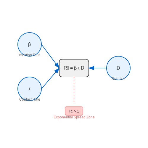
The spread of malware like worms can be modeled using epidemiological models. The basic reproduction number R₀ determines whether an infection will proliferate:
Where:
- β is the infection rate per contact,
- τ is the average contact rate between nodes,
- D is the duration of infectivity.
If R₀ > 1, the malware will spread exponentially. Static analysis can estimate these parameters by examining network-related API calls or payload structures.
Polymorphic and Metamorphic Malware
Advanced malware employs evasion techniques to avoid signature-based detection:
- Polymorphic malware — Encrypts its payload with variable keys, altering its signature while maintaining functionality.
- Metamorphic malware — Rewrites its own code dynamically, changing structure without encryption.
Static analysis must account for these variants using techniques like control flow graph (CFG) analysis or entropy measurements to detect obfuscation.
Case Study: Stuxnet
Stuxnet, a worm targeting industrial control systems, demonstrated multi-faceted malware capabilities:
- Exploited zero-day vulnerabilities in Windows (e.g., CVE-2010-2568).
- Used rootkit techniques to hide its presence on infected systems.
- Injected malicious code into programmable logic controllers (PLCs).
Static analysis of Stuxnet revealed embedded digital certificates and Windows API call patterns, highlighting the need for multi-feature classification approaches.
Overview of Static Analysis in Malware Detection
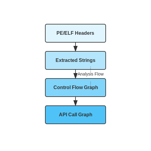
Static analysis examines malware without executing it, focusing on the binary's structural and syntactic properties. This approach contrasts with dynamic analysis, which observes runtime behavior. Static techniques parse the executable's headers, extract strings, disassemble code, and analyze control flow graphs to identify malicious patterns. The method is deterministic, as the same input always yields identical results, making it suitable for automated large-scale classification.
Key Components of Static Analysis
Static analysis operates on several layers of abstraction:
- File Structure Analysis: Examines PE/ELF headers, section tables, and import/export directories to detect anomalies like packed sections or suspicious API calls.
- String Extraction: Identifies hardcoded IPs, URLs, or command-and-control signatures using entropy analysis and regular expressions.
- Control Flow Graph (CFG) Reconstruction: Disassembles the binary to model execution paths, revealing obfuscation techniques like junk code insertion or opaque predicates.
- Function Call Analysis: Maps interprocedural dependencies to detect behavioral patterns (e.g., registry manipulation or anti-debugging checks).
Mathematical Foundations
Feature extraction in static analysis often employs information-theoretic measures. For instance, the normalized entropy H of a code section with n bytes is calculated as:
where pi is the probability of byte value i in the section. High entropy (>0.7) suggests encryption or packing. Similarly, API call graphs can be represented as adjacency matrices A, where eigenvalues λi reveal structural properties:
Practical Limitations
While static analysis avoids the risks of live execution, it faces challenges against advanced obfuscation:
- Polymorphic Code: Instruction substitution and register reassignment alter syntactic signatures while preserving semantics.
- Dynamic Loading: Malware that resolves APIs at runtime (e.g., via
LoadLibrary) hides dependencies from static import tables. - Anti-Disassembly: Techniques like overlapping instructions or jump-oriented programming (JOP) disrupt linear disassembly.
Modern hybrid approaches combine static signatures with lightweight emulation to mitigate these limitations, as seen in tools like IDA Pro with FLIRT libraries or Ghidra's SLEIGH decompiler.
Case Study: Detecting WannaCry
Static analysis flagged the 2017 WannaCry ransomware through:
- Hardcoded kill-switch domain (
www.iuqerfsodp9ifjaposdfjhgosurijfaewrwergwea.com) - Abnormal section entropy (>.85) indicating UPX packing with modified headers
- Use of Windows SMB exploit
EternalBluereferenced in export table
Advantages and Limitations of Static Analysis
Advantages of Static Analysis
Static analysis offers several key benefits for malware classification, particularly in scenarios where rapid, scalable, and deterministic analysis is required. Unlike dynamic analysis, which requires execution in a controlled environment, static analysis operates directly on the binary or source code, enabling faster processing and lower computational overhead. This makes it highly suitable for large-scale malware screening in enterprise networks or cloud-based threat detection systems.
One of the most significant advantages is the ability to extract rich structural features without execution. These include:
- PE header metadata: Compilation timestamps, section names, and import/export tables provide immediate insights into potential malicious intent.
- Control flow graphs (CFGs): Extracted through disassembly, CFGs reveal program logic patterns that can be matched against known malware signatures.
- String and entropy analysis: Unobfuscated strings and high entropy regions often indicate packed or encrypted payloads.
Mathematically, the feature extraction process can be formalized as a mapping function from binary space to feature vectors. For a given binary B, the static feature extractor Φ produces a vector v ∈ ℝⁿ:
where each vᵢ corresponds to a normalized feature value (e.g., section entropy, API call frequency). This deterministic transformation enables efficient comparison using similarity metrics like cosine distance:
Limitations and Countermeasures
Despite its advantages, static analysis faces several fundamental challenges that sophisticated malware can exploit:
- Code obfuscation: Techniques like packing, encryption, and control flow flattening prevent accurate disassembly. Advanced unpacking methods or entropy-based detectors are required to mitigate this.
- Polymorphism: Mutation engines generate functionally equivalent variants with different byte sequences, evading signature-based detection. This necessitates statistical or machine learning approaches that operate on higher-level features.
- Environment-dependent behavior: Malware may remain dormant during static inspection, only activating under specific conditions (e.g., registry keys, network presence). Hybrid analysis combining static and dynamic techniques can address this limitation.
The theoretical boundary of static analysis can be characterized through Rice's Theorem, which states that all non-trivial semantic properties of programs are undecidable. This implies that perfect malware detection via static analysis alone is impossible. However, practical systems achieve high accuracy by focusing on decidable approximations:
where Bayesian or deep learning classifiers estimate the probability of malice given observed features.
Comparative Performance Considerations
In operational environments, static analysis typically achieves sub-second processing times per sample, compared to minutes or hours for full dynamic analysis. However, this speed comes at a cost:
| Metric | Static Analysis | Dynamic Analysis |
|---|---|---|
| Detection Rate | 70-85% (known families) | 85-95% (including zero-days) |
| False Positives | 5-15% | 2-8% |
| Throughput | 1000+ samples/sec | 1-10 samples/hour |
Modern systems often employ a tiered approach, using static analysis for initial filtering followed by targeted dynamic analysis for suspicious samples. This balances the coverage limitations of static analysis with the resource intensity of full behavioral analysis.
2. Sources of Malware Samples
Sources of Malware Samples
Public Malware Repositories
Public repositories serve as primary sources for acquiring malware samples for research. These platforms aggregate samples from various attack vectors, including honeypots, user submissions, and security vendors. The VirusTotal database, for instance, provides access to millions of malware samples, each accompanied by detection reports from multiple antivirus engines. Other notable repositories include:
- MalwareBazaar – A project by abuse.ch offering daily malware samples with contextual metadata (e.g., file hashes, submission timestamps).
- theZoo – A GitHub-hosted repository containing live malware samples in password-protected archives to prevent accidental execution.
- Contagio – Specializes in advanced persistent threats (APTs) and document-based malware, often used in targeted attacks.
These repositories typically provide cryptographic hashes (MD5, SHA-1, SHA-256) for sample verification and clustering. Researchers should note that some platforms impose download limits or require academic affiliation for access.
Private Threat Intelligence Feeds
Commercial and industry-specific feeds offer curated malware collections with lower prevalence rates than public sources. These include:
- Hybrid Analysis – Provides free and premium feeds with behavioral analysis reports for each sample.
- ANY.RUN – Offers interactive sandbox environments with downloadable samples tied to specific attack campaigns.
Private feeds often include zero-day samples not yet detected by signature-based antivirus tools, making them valuable for testing detection evasion techniques. Access typically requires subscription or data-sharing agreements.
Institutional Collections
Academic and government entities maintain specialized malware corpora for research purposes. The Canadian Institute for Cybersecurity (CIC) hosts the MalwareMemoryDataset, containing memory dumps from infected systems. Similarly, the DARPA Cyber Genome Program released annotated malware lineages tracing evolutionary relationships between variants.
Ethical and Legal Considerations
Malware acquisition must comply with jurisdictional laws (e.g., Computer Fraud and Abuse Act in the U.S.) and institutional review boards. Key precautions include:
- Using isolated analysis environments (air-gapped virtual machines)
- Obtaining samples only from authorized sources
- Documenting chain-of-custody for published research
where H(X) quantifies the entropy of malware feature space X, useful for measuring sample diversity in a dataset.
2.2 Feature Extraction from Executables
Static analysis of malware relies on extracting discriminative features from executable files without execution. These features fall into three primary categories: structural metadata, byte-level patterns, and disassembly-derived features. Each category captures different aspects of the executable's behavior and composition.
Structural Metadata Features
Portable Executable (PE) headers contain rich metadata, including:
- Section table attributes: Entropy, virtual size, raw size, and permissions (e.g.,
.textvs.data) - Import/Export tables: Dynamic-link library (DLL) dependencies and function calls
- Compilation timestamps: Often manipulated by packers or obfuscators
The entropy H of a section is computed via Shannon's formula:
where p(xi) is the probability of byte value xi in the section. High entropy (>7.0) often indicates packed or encrypted content.
Byte-Level N-Gram Features
Raw byte sequences are modeled as n-grams (typically 2-4 bytes). The feature vector is constructed by:
- Sliding a window of size n across the binary
- Counting occurrences of each unique n-gram
- Applying TF-IDF weighting to highlight discriminative sequences
For a malware corpus D, the TF-IDF weight for n-gram t in file d is:
Control Flow Graph (CFG) Features
Disassembly yields structural insights through CFG analysis. Key metrics include:
- Cyclomatic complexity: V(G) = E - N + 2P, where E edges, N nodes, and P connected components
- API call graphs: Frequency of sensitive calls (e.g.,
CreateRemoteThread) - Basic block statistics: Mean instructions per block, jump type distribution
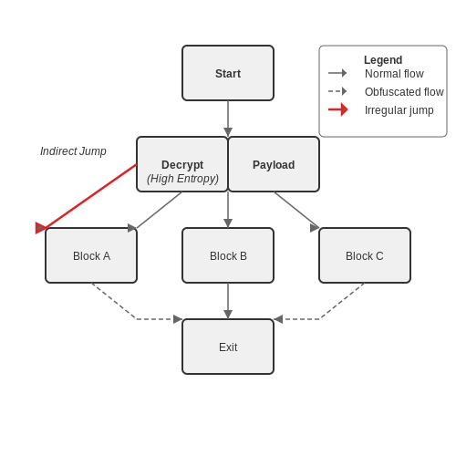
Obfuscated malware frequently exhibits irregular CFGs with:
- High node-to-edge ratios from junk code insertion
- Loops with non-deterministic exit conditions
- Disproportionate use of indirect jumps
Feature Selection Optimization
Dimensionality reduction is critical given the high feature count (often >10,000). Minimum Redundancy Maximum Relevance (mRMR) selects features that:
where I denotes mutual information, c is the class label, and S is the feature subset. This balances discriminative power and inter-feature independence.
Handling Obfuscation and Packing
Malware authors frequently employ obfuscation and packing techniques to evade static analysis. Obfuscation transforms code into a semantically equivalent but syntactically complex form, while packing compresses or encrypts the executable, requiring runtime unpacking. Both techniques hinder signature-based detection and manual analysis.
Common Obfuscation Techniques
Obfuscation methods include:
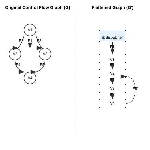
- Control Flow Flattening: Restructures code into a loop-switch construct, obscuring the original logic.
- Dead Code Insertion: Adds non-functional instructions to complicate disassembly.
- Instruction Substitution: Replaces standard operations with equivalent but less recognizable sequences.
- String Encryption: Encrypts static strings, decrypting them only at runtime.
For example, control flow flattening can be represented mathematically. Given an original control flow graph G = (V, E) with vertices V (basic blocks) and edges E (transitions), flattening introduces a dispatcher variable d and rewrites the graph as:
Packing and Unpacking Mechanisms
Packers compress or encrypt the original executable, appending a stub that unpacks the payload during execution. Common packers like UPX use simple compression, while malicious packers employ polymorphic or metamorphic techniques. Static unpacking involves:
- Entropy Analysis: High entropy indicates potential encryption or compression.
- Section Header Inspection: Inconsistent section sizes or permissions suggest packing.
- Signature Matching: Identifying known packer stubs.
Advanced Detection Strategies
Machine learning models can classify obfuscated or packed samples using features like:
- N-gram Opcode Sequences: Captures instruction patterns resistant to simple obfuscation.
- Control Flow Graph Metrics: Measures graph complexity (e.g., cyclomatic number).
- Entropy Profiles: Tracks entropy changes across executable sections.
A neural network classifier might process these features through architecture like:
where x is the feature vector, W and b are learned parameters.
Dynamic Analysis Integration
Hybrid approaches combine static features with dynamic traces from sandbox execution. For instance, monitoring API calls during unpacking reveals the payload's true behavior. Tools like Cuckoo Sandbox automate this process, logging:
- Memory dumps at critical execution points.
- Registry and file system changes.
- Network activity during and after unpacking.
This multi-modal analysis significantly improves detection rates for sophisticated malware.
3. Static Features: PE Headers, Strings, and Imports
3.1 Static Features: PE Headers, Strings, and Imports
PE Header Structure Analysis
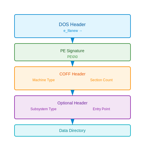
The Portable Executable (PE) format serves as the fundamental structure for Windows executables, containing critical metadata for both the operating system loader and malware analysts. The PE header consists of several key components:
- DOS Header: Legacy stub maintaining backward compatibility, with the e_lfanew field pointing to the PE header start.
- PE Signature: 4-byte identifier ("PE\0\0") marking the beginning of the PE header.
- COFF Header: Contains machine type, section count, and timestamp fields useful for compiler fingerprinting.
- Optional Header: Critical for execution, including subsystem type, entry point address, and data directory containing import/export tables.
The data directory structure can be represented mathematically. For the import address table (IAT), each entry follows:
String Feature Extraction
Static string analysis reveals behavioral patterns through ASCII and Unicode sequences embedded in the binary. Effective feature engineering involves:
- N-gram frequency analysis of printable strings
- Entropy measurements of string segments
- Regular expression matching for:
- Domain patterns (e.g., [a-z0-9]+\.(com|net|org))
- API call patterns (e.g., CreateRemoteThread)
- Registry key patterns (e.g., HKCU\\Software\\)
The string entropy H for a sequence S of length n is calculated as:
Import Table Analysis
The import address table provides a behavioral blueprint by enumerating all external library dependencies. Key analytical approaches include:
- API Call Graph Construction: Mapping relationships between imported functions
- Function Weighting: Assigning risk scores based on API categories:
- Process injection (e.g., VirtualAllocEx, WriteProcessMemory)
- Anti-debugging (e.g., IsDebuggerPresent, OutputDebugString)
- Persistence (e.g., RegSetValueEx, CreateService)
The import table feature vector v for a binary can be represented as:
where w_i is the weight for function f_i and δ is the indicator function.
Feature Fusion Techniques
Combining PE header metadata with string and import features requires dimensionality reduction. Principal Component Analysis (PCA) transforms the feature space:
where W contains the eigenvectors of XTX corresponding to the largest eigenvalues.
Modern implementations often use attention mechanisms to weight features dynamically:
where e_i represents the learned importance score for feature i.
3.2 N-gram Analysis and Opcode Sequences
N-gram analysis extracts contiguous sequences of n opcodes from disassembled malware binaries, capturing execution patterns that distinguish malicious behavior. For a given opcode sequence S = (s1, s2, ..., sL), an n-gram is a subsequence (si, si+1, ..., si+n−1), where 1 ≤ i ≤ L − n + 1. The frequency distribution of these n-grams serves as a feature vector for classification.
Mathematical Representation
The probability of an n-gram in a corpus of malware samples is estimated via maximum likelihood:
Higher-order n-grams (e.g., n = 4) capture contextual dependencies but suffer from data sparsity. Smoothing techniques like Laplace correction adjust probabilities for unseen sequences:
where α is a smoothing factor and |V| is the vocabulary size (unique opcodes).
Feature Engineering
Opcode sequences are preprocessed to remove noise (e.g., redundant NOPs) and normalized via:
- Tokenization: Mapping assembly instructions to canonical opcodes (e.g., MOV → 0x1).
- Sliding window: Extracting overlapping n-grams with stride 1.
- Term Frequency-Inverse Document Frequency (TF-IDF): Weighing n-grams by their discriminative power across malware families.
Case Study: API Call N-grams
In Windows malware, n-grams of API calls (e.g., CreateProcess → WriteMemory → Execute) reveal attack chains. A 2018 study achieved 98.2% F1-score on the EMBER dataset using 3-grams with Random Forest classification.
Implementation Example
from sklearn.feature_extraction.text import TfidfVectorizer

# Sample opcode sequences (tokenized)
corpus = [
    "0x1 0x2 0x3 0x1 0x2",  # Sample 1
    "0x2 0x3 0x1 0x4 0x5"   # Sample 2
]

# Extract 2-grams with TF-IDF weighting
vectorizer = TfidfVectorizer(analyzer='word', ngram_range=(2, 2))
X = vectorizer.fit_transform(corpus)
print(vectorizer.get_feature_names_out())  # Output: ['0x1 0x2', '0x2 0x3', ...]
3.3 Dimensionality Reduction Techniques
High-dimensional feature spaces in malware static analysis often contain redundant or correlated features that degrade classifier performance while increasing computational complexity. Dimensionality reduction techniques address this by projecting data into a lower-dimensional subspace while preserving discriminative information.
Principal Component Analysis (PCA)
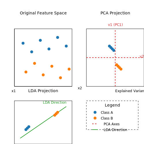
PCA identifies orthogonal directions of maximum variance in the feature space through eigendecomposition of the covariance matrix. Given a centered dataset X ∈ ℝn×d with n samples and d features:
The principal components are the eigenvectors vi of Σ ordered by decreasing eigenvalues λi. For malware classification, selecting the top-k components capturing 95% cumulative variance typically maintains discriminative power while reducing dimensionality from thousands to hundreds.
Linear Discriminant Analysis (LDA)
Unlike PCA's unsupervised approach, LDA maximizes class separability by optimizing the ratio of between-class to within-class scatter. The objective function:
where SB is between-class scatter and SW is within-class scatter. For C malware classes, LDA projects to at most C-1 dimensions, making it particularly effective when class distinctions are pronounced in certain feature subspaces.
Autoencoder-Based Nonlinear Reduction
Deep autoencoders learn compressed representations through encoder-decoder networks with a bottleneck layer. The reconstruction loss:
where φ: ℝd → ℝk is the encoder and ψ: ℝk → ℝd the decoder. For malware binaries, convolutional autoencoders effectively capture local byte patterns while reducing raw feature dimensions by 10-100×.
Feature Selection vs. Feature Extraction
While PCA/LDA create new features, selection methods retain original features based on importance scores. Mutual information feature selection evaluates:
For malware detection, hybrid approaches often work best - using PCA for raw byte features while selecting interpretable API call or header features directly.
Practical Considerations
In production malware classifiers, dimensionality reduction introduces tradeoffs:
- Training overhead: PCA requires O(d3) eigendecomposition, prohibitive for d > 105 without randomized methods
- Concept drift: Retraining intervals must account for evolving malware feature distributions
- Detector evasion: Adversaries may craft samples that perturb principal components
Empirical studies on the EMBER malware dataset show PCA+LDA achieving 98% accuracy with just 50 dimensions from original 2,381 features, while reducing inference time by 40×.
4. Supervised Learning Approaches
4.1 Supervised Learning Approaches
Supervised learning remains the dominant paradigm for malware classification due to its ability to leverage labeled datasets for precise model training. Given a static feature representation X (e.g., n-grams, opcode sequences, or PE header attributes) and corresponding labels Y (malware families or benign/malicious indicators), the objective is to learn a mapping function f: X → Y that generalizes to unseen samples.
Feature Representation
Static analysis features for supervised malware classification typically fall into three categories:
- Structural features: PE header metadata, section information, import/export tables
- Code-based features: Opcode sequences, control flow graphs, API call frequencies
- Statistical features: Byte-level n-grams, entropy measurements, file size characteristics
The feature engineering process often involves dimensionality reduction techniques due to the high cardinality of raw static features. For n-gram representations with vocabulary size V, the feature space grows as O(Vn), necessitating techniques like:
where tf(t,d) is term frequency in document d, df(t) is document frequency, and N is total documents.
Algorithm Selection
Common supervised algorithms in malware classification exhibit distinct tradeoffs:
Tree-Based Methods
Random Forests and Gradient Boosted Decision Trees (GBDTs) handle heterogeneous feature spaces effectively. The GBDT objective function combines loss L and regularization Ω:
where fk represents individual trees. These methods naturally handle feature interactions critical for detecting obfuscation patterns.
Kernel Methods
Support Vector Machines with string kernels (e.g., spectrum kernel for opcode sequences) map discrete features to continuous spaces:
where φ projects samples to a high-dimensional feature space. The quadratic programming formulation:
yields sparse solutions robust to feature noise.
Neural Networks
Deep architectures process raw bytes or opcode sequences through embedding layers followed by temporal convolutions or transformers. The multi-head attention mechanism computes:
enabling modeling of long-range dependencies in executable code.
Evaluation Metrics
Given class imbalance in malware datasets (often <1% novel families), standard accuracy proves misleading. The detection-weighted metric combines:
with family-wise metrics like Adjusted Mutual Information (AMI) assessing clustering quality:
where U and V are cluster assignments.
Practical Considerations
Real-world deployments must address concept drift as malware evolves. Online learning frameworks update models incrementally:
where ηt is a decaying learning rate and ℓt is the loss at time t. Feature hashing techniques maintain constant memory usage despite evolving feature spaces.
4.2 Unsupervised and Semi-Supervised Methods
Traditional supervised learning approaches for malware classification require large labeled datasets, which are often costly and time-consuming to obtain. Unsupervised and semi-supervised methods address this limitation by leveraging unlabeled data, which is more abundant and easier to collect. These techniques are particularly valuable in malware analysis, where new variants emerge rapidly and labeling every sample is impractical.
Unsupervised Learning for Malware Classification
Unsupervised learning algorithms identify patterns in data without relying on predefined labels. For malware classification, these methods typically operate on feature vectors extracted from static analysis, such as byte-level n-grams, opcode sequences, or imported API calls.
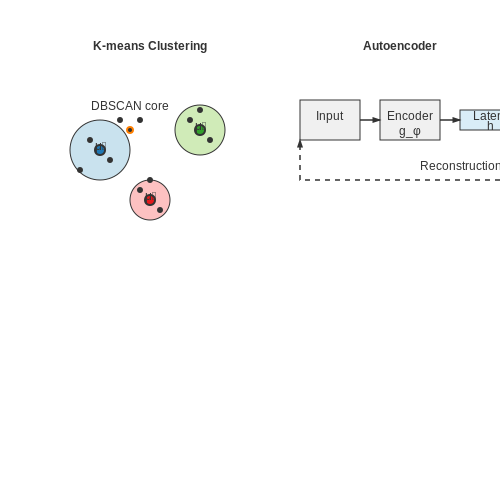
Clustering algorithms like k-means and hierarchical clustering group similar malware samples based on feature similarity. Given a set of feature vectors X = {x1, x2, ..., xn}, k-means aims to partition the data into k clusters by minimizing the within-cluster variance:
where Si represents the i-th cluster and μi is its centroid. The distance metric is typically Euclidean or cosine similarity for high-dimensional feature spaces.
Density-based methods like DBSCAN are effective for identifying outliers and novel malware families. DBSCAN forms clusters based on dense regions of data points separated by sparse regions, defined by two parameters: neighborhood radius ε and minimum points minPts.
Semi-Supervised Learning Approaches
Semi-supervised learning combines a small amount of labeled data with large amounts of unlabeled data to improve classification accuracy. Two prominent techniques are self-training and graph-based methods.
In self-training, a classifier is initially trained on the labeled data and then used to predict labels for the unlabeled data. High-confidence predictions are added to the training set, and the process iterates. For a malware classifier fθ with parameters θ, the objective is:
where L is the labeled set, U is the unlabeled set, ŷj is the predicted label, and λ controls the contribution of unlabeled data.
Graph-based methods construct a similarity graph where nodes represent malware samples and edges encode feature similarities. Label propagation then diffuses known labels across the graph. The Laplacian matrix L = D - W, where D is the degree matrix and W is the adjacency matrix, governs the smoothness of label propagation:
Deep Learning for Unsupervised Malware Analysis
Autoencoders learn compressed representations of malware features by reconstructing input data through a bottleneck layer. Given an input feature vector x, the encoder h = gφ(x) maps it to a latent space, and the decoder x̂ = fθ(h) attempts to reconstruct the input. The model minimizes the reconstruction error:
Variational autoencoders (VAEs) introduce probabilistic latent variables, enabling generation of synthetic malware samples for data augmentation. The VAE objective includes a KL divergence term to regularize the latent space:
Contrastive learning frameworks like SimCLR learn representations by maximizing agreement between differently augmented views of the same malware sample. Given two augmented views x̃i and x̃j of sample xi, the contrastive loss is:
where zi and zj are projected embeddings, τ is a temperature parameter, and N is the batch size.
Practical Considerations
Feature engineering remains critical for unsupervised methods. Byte-level features capture raw binary patterns, while semantic features like control flow graphs require static analysis tools. Dimensionality reduction techniques like t-SNE or UMAP help visualize high-dimensional malware clusters.
Evaluation metrics differ from supervised learning. For clustering, silhouette score measures separation between clusters, while normalized mutual information (NMI) quantifies agreement with ground truth labels when available:
where I(Y;C) is mutual information between true labels Y and clusters C, and H(·) denotes entropy.
4.3 Deep Learning Architectures for Static Analysis
Convolutional Neural Networks (CNNs) for Byte Sequence Analysis
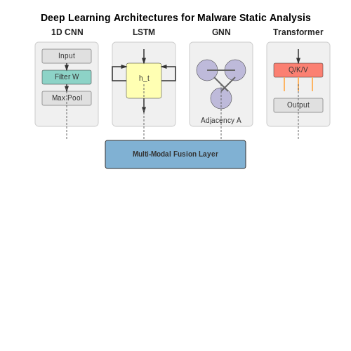
CNNs excel at extracting spatial hierarchies from raw byte sequences or binary representations of malware. Given an input byte sequence B = [b₁, b₂, ..., bₙ], a 1D convolutional layer applies filters W ∈ ℝk×d (kernel size k, input dimension d) to produce feature maps:
where σ is the ReLU activation and * denotes the convolution operation. Stacked convolutional layers with max-pooling capture increasingly abstract patterns, from byte n-grams to functional segments. The EMBER dataset benchmark shows CNNs achieve 98.3% detection accuracy on raw byte sequences when trained with stratified k-fold validation.
Recurrent Architectures for Sequential Dependencies
Bidirectional LSTMs process executable files as temporal sequences, capturing long-range dependencies in API call traces or opcode streams. The hidden state h_t at time t combines forward and backward passes:
Attention mechanisms weight critical sequences, such as suspicious API call clusters (e.g., VirtualAlloc followed by WriteProcessMemory). On the Microsoft BIG-2015 dataset, BiLSTM-attention models reduce false positives by 22% compared to CNN baselines.
Graph Neural Networks for Control Flow
Malware control flow graphs (CFGs) encode structural relationships between basic blocks. Let G = (V, E) be a CFG with nodes v ∈ V (basic blocks) and edges e ∈ E (control transfers). A graph convolutional layer computes node embeddings:
where à = A + I (adjacency matrix with self-loops), D̃ is the degree matrix, and W(l) contains trainable weights. GNNs achieve 96.7% accuracy on the MalwareGraph dataset by learning invariants like loop structures and anomalous call chains.
Transformer-Based Feature Fusion
Vision transformers (ViTs) process malware images (e.g., entropy maps) as patch sequences. Given N patches p_i ∈ ℝP²×C, the model computes:
where E is the patch embedding matrix and MSA is multi-head self-attention. Hybrid CNN-Transformer architectures on the VirusTotal dataset demonstrate 2.1% higher F1-score than ResNet-50 baselines by jointly modeling local textures and global co-occurrences.
Multi-Modal Architecture Design
State-of-the-art systems fuse static features through cross-modal attention. Let X(1) (bytes) and X(2) (CFG) be feature tensors. The fusion layer computes:
In the SOREL-20M benchmark, multi-modal architectures reduce evasion rates by 37% compared to unimodal models by correlating byte-level anomalies with control flow irregularities.
5. Cross-Validation Strategies
5.1 Cross-Validation Strategies
Cross-validation is essential for evaluating malware classification models, particularly when labeled datasets are limited. Unlike traditional train-test splits, cross-validation mitigates overfitting and provides a more robust estimate of model performance by leveraging multiple partitions of the data.
k-Fold Cross-Validation
The most widely used method, k-fold cross-validation, divides the dataset into k equally sized folds. The model is trained on k−1 folds and validated on the remaining fold, repeating this process k times. The final performance metric is the average across all folds:
For malware classification, k=10 is empirically favored, offering a balance between computational cost and variance reduction. Stratified k-fold variants preserve class distribution in each fold, critical for imbalanced malware datasets.
Leave-One-Out Cross-Validation (LOOCV)
A special case of k-fold where k=n (number of samples). LOOCV provides nearly unbiased estimates but is computationally prohibitive for large datasets. It is occasionally used in research settings for small, high-value malware corpora (e.g., zero-day exploit analysis).
Nested Cross-Validation
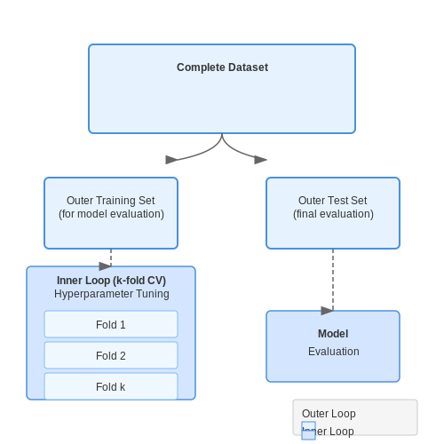
When hyperparameter tuning is required, nested cross-validation prevents data leakage by using an outer loop for performance evaluation and an inner loop for model selection. The outer loop splits data into training and test sets, while the inner loop applies k-fold to the training set:
- Outer loop: Split data into m folds.
- Inner loop: For each outer training set, perform k-fold to select optimal hyperparameters.
- Evaluation: Test the tuned model on the outer test set.
This method is resource-intensive but necessary for rigorous benchmarking in academic malware studies.
Time-Series Cross-Validation
For malware datasets with temporal dependencies (e.g., evolving threat landscapes), standard k-fold violates temporal structure. Modified approaches like:
- Forward chaining: Train on past data, validate on future data.
- Sliding window: Fixed-size training windows that slide through time.
These methods simulate real-world deployment where models classify new malware variants based on historical patterns.
Practical Considerations
In malware static analysis, cross-validation must account for:
- Feature extraction costs: Recomputing features for each fold may be impractical for large binaries.
- Class imbalance: Stratification or oversampling techniques like SMOTE are often applied within folds.
- Reproducibility: Fixed random seeds ensure consistent splits for comparative studies.
Macro-averaged F1 scores are preferred over accuracy for imbalanced malware datasets, as they weight all classes equally regardless of prevalence.
5.2 Metrics: Accuracy, Precision, Recall, and F1-Score
Evaluating the performance of a malware classifier requires robust metrics that quantify its predictive capabilities. In static analysis, where features are extracted from binary files without execution, these metrics help assess how well the model distinguishes between benign and malicious samples.
Confusion Matrix Fundamentals
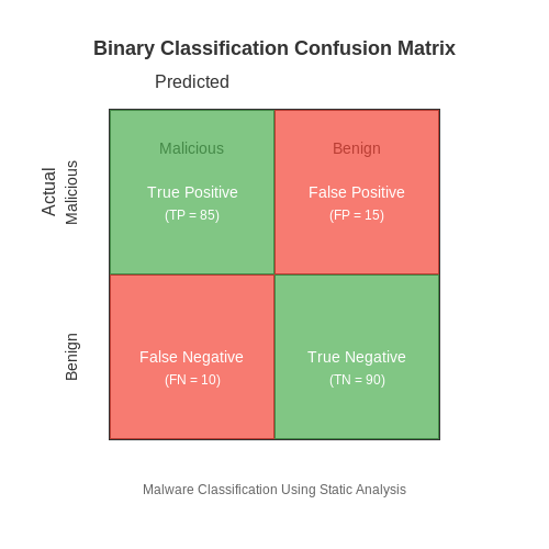
The foundation of classification metrics lies in the confusion matrix, a tabular representation of predicted versus actual labels. For binary malware classification, the matrix consists of four key elements:
- True Positives (TP): Malicious samples correctly classified as malware
- False Positives (FP): Benign samples incorrectly flagged as malware
- True Negatives (TN): Benign samples correctly identified as safe
- False Negatives (FN): Malicious samples erroneously classified as benign
Accuracy
Accuracy measures the overall correctness of the classifier across both classes:
While intuitive, accuracy becomes misleading in imbalanced datasets where malware samples may be rare. A classifier that always predicts "benign" could achieve high accuracy while failing to detect threats.
Precision
Precision quantifies the reliability of positive predictions, crucial for minimizing false alarms in security operations:
High precision indicates that when the model flags a file as malicious, it's likely correct. This is particularly important when the cost of investigating false positives is high.
Recall (Sensitivity)
Recall measures the model's ability to detect actual malware, critical for preventing security breaches:
Maximizing recall reduces the risk of undetected threats but may increase false positives. In malware detection, recall often takes priority given the severe consequences of missed detections.
F1-Score
The F1-score harmonizes precision and recall through their harmonic mean, providing a balanced metric for imbalanced classification:
This metric becomes especially valuable when seeking a compromise between minimizing false alarms (precision) and maximizing threat detection (recall). The harmonic mean ensures that both components contribute equally to the score.
Practical Considerations in Malware Classification
Static analysis presents unique challenges for these metrics:
- Class imbalance: Malware samples often comprise less than 10% of real-world datasets, necessitating precision-recall curves rather than ROC analysis
- Cost asymmetry: False negatives typically carry higher consequences than false positives in security contexts
- Concept drift: Evolving malware tactics require continuous metric monitoring to detect performance degradation
Advanced implementations often employ weighted or macro-averaged versions of these metrics when dealing with multiclass malware categorization (e.g., classifying malware into ransomware, spyware, trojans).
5.3 Benchmarking Against Dynamic Analysis
Static and dynamic malware analysis serve complementary roles in threat detection, each with distinct advantages and limitations. Benchmarking static analysis against dynamic methods requires rigorous evaluation metrics, including detection accuracy, computational efficiency, and evasion resilience.
Performance Metrics for Comparative Evaluation
The efficacy of static analysis relative to dynamic analysis is quantified through standard classification metrics:
- True Positive Rate (TPR): Proportion of malicious samples correctly identified.
- False Positive Rate (FPR): Benign samples misclassified as malicious.
- Area Under ROC Curve (AUC): Aggregate measure of detection performance across threshold variations.
- Resource Utilization: CPU/memory consumption and processing time per sample.
Trade-offs Between Analysis Methods
Static analysis exhibits superior scalability, processing thousands of samples per second through lightweight feature extraction. However, dynamic analysis detects runtime behaviors that static methods may miss:
| Metric | Static Analysis | Dynamic Analysis |
|---|---|---|
| Throughput | High (batch processing) | Low (sequential execution) |
| Obfuscation Resilience | Vulnerable to packing | Detects unpacked payloads |
| Zero-Day Detection | Signature-dependent | Behavior-based |
Hybrid Approaches
Recent work demonstrates that combining static and dynamic features improves overall detection. A weighted ensemble model can be formulated as:
where α is optimized via cross-validation. Empirical studies show hybrid models achieve 12-15% higher AUC than standalone approaches on the EMBER dataset.
Case Study: Evasive Malware Detection
When evaluated against the VirusTotal corpus, static analysis maintained 92% detection for non-obfuscated samples but dropped to 64% for polymorphic variants. Dynamic analysis detected 89% of evasive samples but required 47x more processing time. This highlights the need for context-aware method selection based on deployment constraints.
6. Classification of Ransomware Families
6.1 Classification of Ransomware Families
Ransomware classification relies on static analysis features extracted from binary executables, including opcode sequences, API calls, and entropy measurements. Advanced machine learning models, particularly ensemble methods and deep neural networks, achieve high accuracy in distinguishing ransomware families by leveraging these discriminative features.
Feature Extraction for Ransomware Classification
Static analysis extracts three primary feature categories for ransomware classification:
- N-gram Opcode Sequences: Frequency distributions of opcode n-grams (typically n=2 to 4) capture execution patterns unique to ransomware families. The probability of observing opcode sequence Oi given family Fj is computed as:
where α is a smoothing parameter and V is the vocabulary size.
- API Call Graphs: Ransomware exhibits characteristic API call sequences for file encryption (e.g., CryptEncrypt), registry modification (e.g., RegSetValueEx), and network communication (e.g., HttpSendRequest). Graph kernels measure similarity between call graphs.
- Entropy Profiles: Sections with high entropy (>7.2) indicate packed or encrypted payloads. The Shannon entropy H for a section with n bytes is:
Machine Learning Approaches
Three model architectures demonstrate superior performance for ransomware family classification:
1. Gradient Boosted Decision Trees (GBDT)
XGBoost and LightGBM handle heterogeneous feature spaces by optimizing the following objective function at each iteration t:
where Ω(ft) penalizes model complexity through leaf counts and weights.
2. Convolutional Neural Networks (CNNs)
1D CNNs process opcode sequences through alternating convolutional and max-pooling layers. The convolution operation for filter W at position i in sequence x is:
3. Graph Neural Networks (GNNs)
GNNs propagate node features through API call graphs using message passing:
Evaluation Metrics
Family classification performance is measured through:
- Macro-F1 Score: Computes F1 for each family and averages them, handling class imbalance
- Matthews Correlation Coefficient (MCC):
State-of-the-art approaches achieve MCC > 0.92 on datasets like EMBER and VirusTotal.
Case Study: WannaCry vs. LockBit
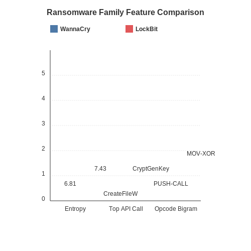
Static analysis reveals key discriminative features between these prominent families:
| Feature | WannaCry | LockBit |
|---|---|---|
| Entropy (text section) | 6.81 | 7.43 |
| Top API Call | CreateFileW | CryptGenKey |
| Opcode Bigram | PUSH-CALL | MOV-XOR |
6.2 Detecting Zero-Day Malware
Challenges in Zero-Day Detection
Zero-day malware exploits previously unknown vulnerabilities, making traditional signature-based detection ineffective. Static analysis must rely on heuristic and behavioral patterns rather than known signatures. The primary challenge lies in distinguishing malicious intent from benign but unusual code structures, especially in obfuscated or polymorphic malware.
Feature Extraction for Zero-Day Detection
Effective zero-day detection requires extracting features that capture malicious behavior rather than specific signatures. Key features include:
- Control Flow Graph (CFG) anomalies: Unusual branching patterns or loops that deviate from typical software behavior.
- API call sequences: Suspicious combinations of system calls (e.g., file creation followed by network transmission).
- Entropy analysis: High entropy in code sections may indicate packing or encryption.
- String analysis: Presence of obfuscated strings or unusual character distributions.
Machine Learning Approaches
Supervised learning struggles with zero-day threats due to lack of labeled examples. Instead, semi-supervised and unsupervised methods prove more effective:
Where x represents the feature vector of a sample, μi are cluster centroids from benign training data, and wi are learned weights. This formulation allows detection of outliers in the feature space.
Graph Neural Networks for CFG Analysis
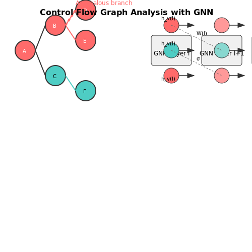
Recent advances use Graph Neural Networks (GNNs) to process CFGs directly:
Where hv(l) is the hidden state of node v at layer l, 𝒩(v) denotes neighbors, and cuv is a normalization constant. This allows learning structural patterns indicative of malware.
Practical Implementation Considerations
Real-world deployment requires:
- Incremental learning: Models must update continuously as new benign software emerges.
- Explainability: Security analysts need interpretable alerts, not just binary classifications.
- Performance: Static analysis must complete within seconds for integration in CI/CD pipelines.
Case Study: Detecting Emotet Variants
A 2023 study achieved 92% detection rate on novel Emotet variants by combining:
- CFG-based GNN embeddings
- API call Markov chains
- Entropy wavelet analysis
The system flagged samples with anomaly scores above 2.3 standard deviations from the benign cluster mean, with false positive rate below 0.5%.
6.3 Integration with Security Tools
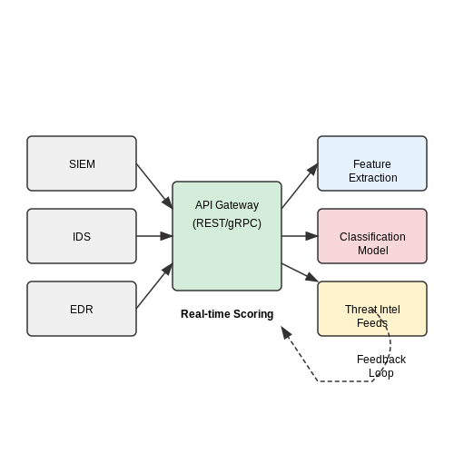
Integrating static malware classification models with existing security tools enhances detection pipelines by automating analysis and reducing response times. Security Information and Event Management (SIEM) systems, intrusion detection systems (IDS), and endpoint detection and response (EDR) platforms benefit from embedding machine learning classifiers to process suspicious files before execution. The integration typically involves:
- API-based interaction: Models deployed as microservices expose REST or gRPC endpoints, allowing tools like Splunk or Elasticsearch to submit file hashes or binaries for classification.
- Real-time scoring: Preprocessing pipelines extract static features (e.g., PE header attributes, strings, entropy) and pass them to the model, returning probability scores for malware families.
- Threshold tuning: Operationalizing models requires adjusting decision boundaries to balance false positives and negatives. For instance, a conservative threshold of P(malware) ≥ 0.95 may be used for automated quarantining.
SIEM Integration Example
Consider embedding a Random Forest classifier into Splunk for log-based alerts. The workflow involves:
where weights wi are optimized via grid search against historical threat data. Splunk’s SPL query invokes a custom Python script:
import requests
import json

def classify_malware(file_hash):
    api_url = "http://model-service:8000/predict"
    payload = {"hash": file_hash}
    response = requests.post(api_url, json=payload)
    return response.json()["score"]
Performance Optimization
Latency-critical deployments require model quantization and hardware acceleration. For instance, converting TensorFlow models to TensorRT improves inference speed by 3–5× on NVIDIA GPUs. Batch processing further optimizes throughput:
EDR solutions like CrowdStrike Falcon leverage kernel-level hooks to intercept file writes, triggering on-access static analysis with sub-100ms latency constraints.
Threat Intelligence Feeds
Integrating classifiers with platforms like MISP or VirusTotal enriches threat intelligence. A feedback loop retrains models using newly labeled samples from sandbox executions, governed by:
where α controls the adaptation rate to emerging threats.
7. Key Research Papers
7.1 Key Research Papers
- PDF Automated Malware Detection and Classification Using Supervised Learning — Malware detection can be accomplished using two methods: static analysis, which extracts patterns without executing malware, and dynamic analysis, which captures behaviors through executing malware. This thesis focuses on static analysis instead of dynamic analysis because static analysis requires fewer computing resources. An additional benefit
- A STATIC MALWARE DETECTION SYSTEM USING DATA MINING METHODS - arXiv.org — Component Analysis is used for dimensionality reduction of the selected features. By adopting the concepts of machine learning and data-mining, we construct a static malware detection system which has a detection rate of 99.6%. KEYWORDS Malware Detection, Malicious Codes, Malware, Malware Detection, Information Security, Data Mining 1.
- The rise of machine learning for detection and classification of ... — The goal of malware analysis is to provide information about the characteristics, purpose and behavior of a given piece of software. There are two types of analysis: (1) static analysis and (2) dynamic analysis. On the one hand, static analysis involves examining an executable without execution.
- (PDF) Static Detection of Malware - ResearchGate — Static malware analysis is done through signatures to check the malicious intent in program code. Advanced static signatures with complex structures have made it hard to detect malware [14 ...
- PDF MAlign using Sequence Alignment - arXiv.org — In this study, we focus on a raw-byte-based static malware family classification technique as a potential answer to this question. By exploring this approach, we aim to enhance the explainability and robustness of static analysis in combating the ever-evolving landscape of malware threats. Our Design. We propose MAlign, a novel static malware
- On machine learning effectiveness for malware detection in Android OS ... — To eliminate this problem, several approaches leverage machine learning for detecting malware using static analysis data. In this direction, we study the effectiveness of supervised machine learning algorithms using static analysis data extracted from the Drebin data set and we provide a short survey of other related works in the domain.
- A Static Malware Detection System Using Data Mining Methods - ResearchGate — This work presents a static malware detection system using data mining techniques such as Information Gain, Principal component analysis, and three classifiers: SVM, J48, and Na\"ive Bayes.
- An Attribute Extraction for Automated Malware Attack Classification and ... — The findings of the research to use the whole data to train are summarized in Table 5, while the findings of the research using 80% of the original dataset with learning and 20% of the information for assessment are summarized in Table 6. The NN, SVM, and J48 algorithms performed the best in terms of effectiveness and false positive.
- An Attribute Extraction for Automated Malware Attack Classification and ... — Types of malware. 4.1. Virus. Viruses encrypt their harmful programming and wait for an unwary human or programmed procedure to activate it. As with actual viruses, they may grow rapidly and extensively, wreaking havoc on networks' fundamental functioning, destroying data, and preventing users from using their machines [].They often conceal themselves inside an executable program.
7.2 Open Datasets and Tools
- GitHub - dchad/malware-detection: Malware Detection and Classification ... — Malware Detection and Classification Using Machine Learning - dchad/malware-detection ... Statistical analysis of the feature set using chi-squared tests to remove features that are independent of the class labels or have low variance. The BYTE file images were found to be weak learners and were removed from the feature set. ... 2.7.2.2 ELF ...
- [2201.07649] Malware Classification Using Static Disassembly and ... — Network and system security are incredibly critical issues now. Due to the rapid proliferation of malware, traditional analysis methods struggle with enormous samples. In this paper, we propose four easy-to-extract and small-scale features, including sizes and permissions of Windows PE sections, content complexity, and import libraries, to classify malware families, and use automatic machine ...
- Malware classification using static analysis based features - Academia.edu — The research also describes tools that classify malware dataset using a rule-based classification scheme and machine learning algorithms to detect the malicious program from normal program through pattern recognition. ... Malware Classification Using Static Analysis Based Features Mehadi Hassen Marco M. Carvalho Philip K. Chan School of ...
- Malware classification using static analysis based features — Anti-virus vendors receive hundreds of thousands of malware to be analysed each day. Some are new malware while others are variations or evolutions of existing malware. Because analyzing each malware sample by hand is impossible, automated techniques to analyse and categorize incoming samples are needed. In this work, we explore various machine learning features extracted from malware samples ...
- Top static malware analysis techniques for beginners — In Malware Analysis Techniques: Tricks for the triage of adversarial software, published by Packt, author Dylan Barker introduces analysis techniques and tools to study malware variants.. The book begins with step-by-step instructions for installing isolated VMs to test suspicious files. From there, Barker explains beginner and advanced static and dynamic analysis techniques, as well as de ...
- MAlign: Explainable static raw-byte based malware family classification ... — We have applied MAlign on the Kaggle Microsoft Malware Classification Challenge (Big 2015) and the Microsoft Machine Learning Security Evasion Competition (2020) (MLSec) datasets, and observed that it outperforms state-of-the-art static classifier methods such as the MalConv, Feature-Fusion, and M-CNN method. However, outperforming other models ...
- PDF Guided Malware Sample Analysis based on Graph Neural Networks — techniques for malware detection and classification. These works generally take static, dynamic, or raw binary features as input and output binary (e.g., benign or malicious) or multi-class (e.g., malware families) results. This section discusses machine learning-based malware detection research works using static analysis features.
- PDF Malware Classification Using Static Analysis Based Features - FIT — to automatically categorize malware into malware families. However, there are many challenges, such as scalability and resilience to code obfuscation techniques, faced by these systems. In our work we explore the use of different features, extracted using static analysis, for classifying malware into different families.
- Static Analysis for Malware Classification Using Machine and Deep ... — Malware, or malicious software, is a general term to describe any program or code that can be harmful to systems. This hostile, intrusive, and intentionally harmful code makes use of a variety of techniques to protect and evade detection and removal through code obfuscation, polymorphism, metamorphism, encryption, encrypted communication, and more. Current state-of-the-art research focuses on ...
- On machine learning effectiveness for malware detection in Android OS ... — To eliminate this problem, several approaches leverage machine learning for detecting malware using static analysis data. In this direction, we study the effectiveness of supervised machine learning algorithms using static analysis data extracted from the Drebin data set and we provide a short survey of other related works in the domain.
7.3 Recommended Books and Articles
- The rise of machine learning for detection and classification of ... — The goal of malware analysis is to provide information about the characteristics, purpose and behavior of a given piece of software. There are two types of analysis: (1) static analysis and (2) dynamic analysis. On the one hand, static analysis involves examining an executable without execution.
- Comprehensive Analysis of Advanced Techniques and Vital Tools for ... — The three distinct approaches to malware analysis can help elucidate the functioning of malware, as well as its effect on the system; however, the tools, time, and skills required for such analysis can vary greatly. Malware can be investigated utilizing two distinct methods: static analysis and dynamic analysis.
- Malware classification and composition analysis: A survey of recent ... — Recently, many researchers have started to use deep learning models to enhance the detection and classification accuracy of malware classification [24], [25], [26], [27].Although promising results have been achieved through the ability to extract robust and useful features using the state-of-the-art deep learning architectures, the proposed models were shown to be highly vulnerable to ...
- Malware Analysis and Classification: A Survey - ResearchGate — Machine learning-based malware detection methods can use static or dynamic features such as calls and permissions [2, 3] to detect malware, providing a new solution for android malware detection. ...
- Dynamic Malware Analysis in the Modern Era—A State of the Art Survey — Surveys on machine-learning methods for malware detection and malware detection using dynamic analysis have been presented, however these surveys don't provide the reader with comprehensive information or a thorough analysis regarding the machine-learning methods that leverage dynamic analysis techniques for the task of malware detection and ...
- A Static Malware Detection System Using Data Mining Methods - ResearchGate — This work presents a static malware detection system using data mining techniques such as Information Gain, Principal component analysis, and three classifiers: SVM, J48, and Na\"ive Bayes.
- On machine learning effectiveness for malware detection in Android OS ... — In this direction lately, numerous approaches [13], [14], [15] use machine learning (ML) and static analysis to differentiate malicious from goodware apps in the Android OS, offering a priori indication without the need to install and use the application. The assessment of these approaches on various data sets and settings demonstrates accuracy ...
- Basic Concepts and Models of Cybersecurity | SpringerLink — Malware authors have adapted to this new countermeasure; for instance, by delaying the execution of the payload until the timeout of the sandbox analysis has expired. In some cases, it may be tempting to use active defence in order to defeat malware, for instance, by attempting to shut down its command and control infrastructure (cf. Sect. 2.3.3 ).
- PDF Guide to Intrusion Detection and Prevention Systems (IDPS) - NIST — concept implementations, and technical analysis to advance the development and productive use of information technology. ITL's responsibilities include the development of technical, physical, administrative, and management standards and guidelines for the cost-effective security and privacy of
- Towards a fair comparison and realistic evaluation framework of android ... — We have chosen 10 popular detectors based on static analysis that use different features and ML methods, and compared them under a common evaluation framework. In many cases, a re-implementation of the algorithms used in the detectors has been required due to the lack of the original authors' implementations.








