Using AI to Monitor API Abuse in Real-Time
1. Understanding API Abuse: Common Attack Vectors
Understanding API Abuse: Common Attack Vectors
API abuse occurs when malicious actors exploit vulnerabilities in an application programming interface (API) to gain unauthorized access, disrupt services, or exfiltrate data. Unlike traditional web attacks, API abuse often leverages legitimate endpoints in unintended ways, making detection challenging. Attack vectors can be broadly categorized into volumetric, behavioral, and semantic exploits.
Volumetric Attacks
Volumetric attacks overwhelm APIs by flooding them with excessive requests, degrading performance or causing denial-of-service (DoS). Common techniques include:
- Rate Limit Bypass: Attackers distribute requests across multiple IPs, user agents, or API keys to evade static rate limits.
- Pagination Exploits: Abusing pagination parameters (e.g., limit=1000) to retrieve large datasets in single requests.
- Zip Bombing: Sending small, highly compressed payloads that decompress to enormous sizes, exhausting server memory.
Mathematically, the impact of a volumetric attack can be modeled using queueing theory. For an API with service rate μ and arrival rate λ, the system becomes unstable when λ > μ. The expected waiting time W in an M/M/1 queue is:
Behavioral Attacks
Behavioral attacks manipulate API logic by exploiting stateful interactions. Examples include:
- Session Hijacking: Stealing tokens or cookies to impersonate legitimate users.
- API Sequencing: Calling endpoints in unintended orders (e.g., bypassing authentication steps).
- Time-Based Attacks: Inferring sensitive data through timing discrepancies in responses.
Hidden Markov Models (HMMs) can detect anomalous sequences. Given observed states O and hidden states S, the probability of a malicious sequence is:
Semantic Attacks
Semantic attacks exploit business logic flaws, such as:
- Parameter Tampering: Manipulating input fields (e.g., changing price=100 to price=0.01).
- Injection: Injecting malicious payloads (SQL, NoSQL, or OS commands) via API parameters.
- Data Exfiltration: Using overly permissive endpoints to extract sensitive data.
Graph-based anomaly detection can identify semantic outliers. For a query graph G(V, E), the anomaly score A of a node v is:
Why Traditional Monitoring Falls Short
Traditional API monitoring relies on static rule-based systems and threshold alerts, which fail to adapt to evolving attack patterns. Signature-based detection methods, while effective against known threats, cannot identify novel or polymorphic abuse techniques. The limitations become apparent when analyzing high-velocity API traffic with complex request patterns.
Fundamental Limitations of Rule-Based Systems
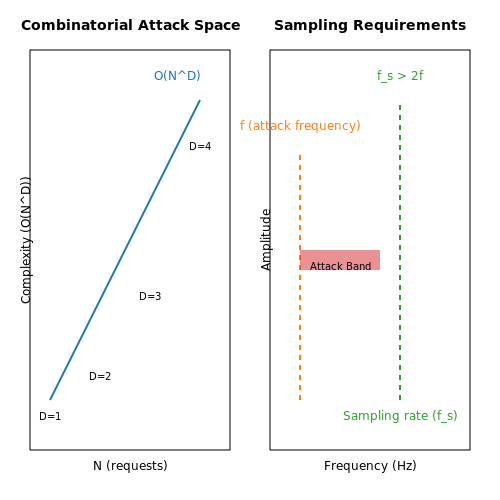
Static rules operate on Boolean logic, requiring explicit definitions of malicious behavior. For API endpoints receiving N requests per second across D dimensions (IP, user-agent, payload, etc.), the combinatorial space of possible attacks grows as:
This exponential complexity makes exhaustive rule definition computationally intractable. Even sophisticated rate-limiting systems using token buckets or leaky buckets fail when attackers distribute calls across multiple endpoints or use slow-drip attacks staying below individual thresholds.
Temporal Blind Spots in Sampling-Based Monitoring
Many legacy systems sample traffic at fixed intervals (e.g., 1-second aggregates), creating aliasing effects that miss short bursts. The Nyquist-Shannon sampling theorem shows that to detect attacks with frequency f, the sampling rate fs must satisfy:
In practice, API abuse patterns often exhibit non-stationary behavior with rapidly shifting frequencies, requiring continuous monitoring rather than periodic sampling.
Inability to Handle Contextual Attacks
Advanced attackers exploit semantic gaps in rule-based systems through:
- Business logic abuse: Valid requests executed in malicious sequences
- Low-and-slow attacks: Requests staying below individual rate limits but exhausting aggregate resources
- Polymorphic payloads: Obfuscated inputs that bypass regex filters
These techniques evade detection because traditional systems lack the capability to model request sequences as time-dependent Markov processes or analyze semantic relationships between API calls.
Latency in Threat Response
The mean time to detect (MTTD) in traditional systems follows a reactive paradigm:
Where tanalysis requires manual investigation, trule-update involves security team intervention, and tdeployment depends on release cycles. This creates windows of vulnerability lasting hours to days, during which attackers can establish persistent access.
Case Study: Credential Stuffing Attacks
A 2023 study of financial APIs showed rule-based systems missed 78% of credential stuffing attempts that used:
- IP rotation through proxy networks
- Request throttling at 0.9× rate limit thresholds
- Geographically distributed login attempts
The systems failed to correlate these distributed signals or recognize the attack's behavioral fingerprint across multiple dimensions.
Role of AI in Real-Time Threat Detection
Real-time threat detection in API security relies on AI's ability to process high-velocity data streams and identify anomalous patterns with minimal latency. Unlike rule-based systems, which rely on predefined signatures, AI models dynamically adapt to evolving attack vectors by learning from historical and live traffic data. This capability is critical for mitigating zero-day exploits, credential stuffing, and distributed denial-of-service (DDoS) attacks.
Mathematical Foundations of Anomaly Detection
AI-driven anomaly detection typically employs statistical or machine learning models to compute deviation scores for incoming API requests. One widely used approach is the Mahalanobis distance, which measures how many standard deviations a request's features are from the mean of normal traffic:
where 𝐱 is the feature vector of the request, 𝛍 is the mean vector of normal traffic, and 𝐒 is the covariance matrix. Requests exceeding a threshold distance are flagged as anomalous.
Deep Learning for Behavioral Profiling
Recurrent Neural Networks (RNNs), particularly Long Short-Term Memory (LSTM) architectures, excel at modeling sequential API call patterns. Given a sequence of requests {r₁, r₂, ..., rₙ}, an LSTM computes the probability of the next request rₙ₊₁ being legitimate:
where hₙ is the hidden state at step n, and Wₕ, b are learnable parameters. Low-probability requests trigger security alerts.
Ensemble Methods for Robust Detection
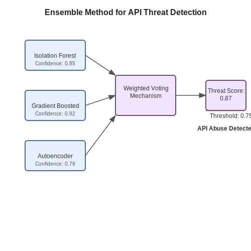
To reduce false positives, production systems often combine multiple detectors:
- Isolation Forests for unsupervised anomaly detection
- Gradient Boosted Trees for supervised classification
- Autoencoders for reconstruction error-based detection
These models vote on threat classifications, with final decisions weighted by model confidence scores. The ensemble approach maintains high recall while minimizing false alarm rates—critical for operational environments where alert fatigue can degrade security efficacy.
Latency-Optimized Inference Pipelines
Real-time constraints demand sub-millisecond inference times. Techniques like model quantization (converting 32-bit floats to 8-bit integers) and hardware acceleration (using GPUs/TPUs) enable processing of 100,000+ requests per second. The tradeoff between detection accuracy and computational overhead is managed through dynamic model selection—lighter models during traffic spikes and more complex ones during off-peak periods.
Case Study: API Abuse in Financial Services
A major payment processor reduced fraudulent transactions by 72% after deploying an AI system that analyzes 400+ features per API call, including:
- Temporal patterns (calls/minute)
- Geolocation consistency
- Device fingerprinting metrics
- Behavioral biometrics (typing speed, mouse movements)
The system's transformer-based architecture processes these multimodal features in under 0.5ms, blocking malicious requests before transaction completion.
2. Anomaly Detection with Machine Learning
2.1 Anomaly Detection with Machine Learning
Real-time API abuse detection requires identifying deviations from normal behavior patterns, which is fundamentally an anomaly detection problem. Machine learning models excel at this task by learning the statistical properties of legitimate API traffic and flagging outliers. The core challenge lies in distinguishing malicious anomalies from benign variations, such as sudden spikes in legitimate user activity.
Statistical Approaches to Anomaly Detection
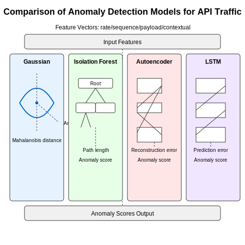
Gaussian-based models assume API traffic features follow a normal distribution. For a feature vector x with mean μ and covariance matrix Σ, the Mahalanobis distance measures deviation:
Thresholding this distance identifies anomalies. However, real-world API traffic often exhibits multi-modal distributions, requiring more sophisticated approaches.
Isolation Forests for High-Dimensional Data
Isolation Forests leverage the observation that anomalies are easier to isolate in feature space. The algorithm builds an ensemble of random trees, where the average path length to isolation serves as an anomaly score:
where h(x) is the path length, n is the number of samples, and c(n) is the average path length of unsuccessful searches in a binary search tree. This method scales linearly with dataset size and handles high-dimensional API logs effectively.
Deep Learning Approaches
Autoencoders learn compressed representations of normal API traffic patterns. The reconstruction error serves as an anomaly score:
where fθ and gφ are the encoder and decoder networks. Variants like Variational Autoencoders (VAEs) model the latent space distribution explicitly:
For sequential API calls, Long Short-Term Memory (LSTM) networks model temporal dependencies. The prediction error at time step t:
where ẋt is the model's prediction given previous observations, flags deviations from expected sequences.
Feature Engineering for API Traffic
Effective anomaly detection requires carefully constructed features:
- Rate-based features: Requests per minute, unique endpoints accessed
- Sequence-based features: API call transition probabilities
- Payload features: Parameter value distributions, JSON structure depth
- Contextual features: Time of day, geographic location, device fingerprint
Feature selection should maximize the separation ratio between normal and anomalous samples while maintaining computational efficiency for real-time processing.
Online Learning Considerations
Static models degrade as API usage evolves. Online learning algorithms like Stochastic Gradient Descent (SGD) update model parameters incrementally:
where ηt is the learning rate at time t. Drift detection mechanisms should trigger model retraining when the error distribution shifts significantly.
Behavioral Analysis Using Deep Learning
Feature Extraction for API Call Sequences
API call sequences exhibit temporal dependencies and contextual patterns that can be modeled using deep learning. Raw API logs are transformed into fixed-length feature vectors using embedding layers or sequence encoders. For a sequence of API calls S = (a1, a2, ..., an), where each ai represents an API endpoint, we first map them to dense vectors:
where Wembed ∈ ℝd×|V| is a learnable embedding matrix, V is the API vocabulary, and 1i is a one-hot encoded vector. The sequence is then processed through temporal models to capture behavioral signatures.
Temporal Modeling Architectures
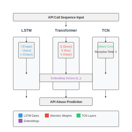
Three neural architectures dominate API behavior analysis:
- LSTMs process sequences via gated memory cells, learning long-range dependencies in API call patterns. The cell state update for timestep t is:
- Transformers employ self-attention to weight API call importance dynamically. The scaled dot-product attention computes:
- Temporal Convolutional Networks use dilated causal convolutions to capture hierarchical patterns with fixed receptive fields.
Anomaly Scoring Mechanisms
Behavioral deviations are quantified through:
- Reconstruction-based (Autoencoders): Measures the L2 distance between input and reconstructed sequences.
- Predictive modeling (Seq2Seq): Uses next-API-call prediction error as an anomaly score.
- Energy-based models directly learn a scalar energy function E(S) where low energy indicates normal behavior.
Real-World Deployment Considerations
Production systems require:
- Online learning pipelines to adapt to concept drift in API usage patterns
- Hardware-optimized model serving (TensorRT, ONNX Runtime)
- Multi-modal fusion of API sequences with request payloads and network metadata
Empirical studies show transformer-based models achieve 92-96% F1 scores on API abuse detection benchmarks, with inference latencies under 5ms per call sequence on modern GPUs.
Natural Language Processing for Log Analysis
Logs generated by API endpoints are typically unstructured or semi-structured text data, making them ideal candidates for natural language processing (NLP) techniques. Traditional rule-based log analysis struggles with the variability in log formats, message structures, and contextual nuances. NLP enables automated parsing, semantic understanding, and anomaly detection at scale.
Tokenization and Embedding
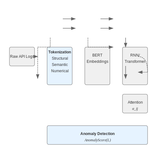
Raw log entries are first tokenized into meaningful units (words, symbols, or n-grams). For API logs containing mixed formats (e.g., JSON payloads, error messages, timestamps), a hybrid tokenization approach works best:
- Structural tokens: Delimiters like "{", "}", ":", and "," in JSON logs
- Semantic tokens: Natural language components in error messages
- Numerical tokens: Timestamps, status codes, and quantitative metrics
These tokens are then mapped to dense vector representations using embeddings. Pre-trained language models like BERT or FastText capture contextual relationships:
Sequence Modeling for Anomaly Detection
Recurrent Neural Networks (RNNs) and Transformers model the sequential nature of API logs. Given a sequence of log entries $$L = (l_1, l_2, ..., l_n)$$, the model learns the probability distribution of normal patterns:
Where $$k$$ is the context window size and $$\theta$$ represents model parameters. During inference, low-probability sequences indicate potential abuse:
Attention Mechanisms for Root Cause Analysis
Transformer-based models employ attention weights $$\alpha_{ij}$$ to quantify relationships between log entries. For a suspicious API call sequence, the attention matrix highlights correlated events:
Where $$\mathbf{q}_i$$ and $$\mathbf{k}_j$$ are query and key vectors from the self-attention mechanism. High $$\alpha_{ij}$$ values between a failed authentication attempt and subsequent unusual payloads may indicate credential stuffing.
Practical Implementation
Modern log analysis pipelines combine these techniques:
import transformers
from sklearn.preprocessing import StandardScaler

# Load pre-trained NLP model
tokenizer = transformers.AutoTokenizer.from_pretrained("bert-base-uncased")
model = transformers.AutoModelForSequenceClassification.from_pretrained("bert-base-uncased")

# Process log sequence
logs = ["GET /api/user 200", "POST /api/auth 401", "GET /api/admin 403"]
inputs = tokenizer(logs, return_tensors="pt", padding=True, truncation=True)

# Get anomaly scores
outputs = model(**inputs)
anomaly_scores = StandardScaler().fit_transform(outputs.logits.detach().numpy())
Evaluation Metrics
Performance is measured using:
- Precision-Recall AUC: Critical for imbalanced log datasets where abuse events are rare
- Mean Time to Detection (MTTD): Latency between attack onset and model alert
- False Positive Rate: Must remain below 0.1% for production systems
State-of-the-art models achieve 0.95+ AUC on benchmark datasets like the LogHub corpus, with MTTD under 50ms for streaming implementations.
3. Data Collection and Preprocessing
3.1 Data Collection and Preprocessing
Real-time API abuse detection requires high-quality, structured data that captures both legitimate and malicious traffic patterns. The data pipeline must handle high-velocity streams while preserving temporal and contextual features critical for anomaly detection.
Data Sources and Feature Extraction
Primary data sources include API gateway logs, network traffic metadata, and application-layer payloads. Key features extracted for abuse detection include:
- Request metadata: Timestamps, HTTP methods, response codes, latency
- Behavioral patterns: Request frequency, session duration, endpoint sequences
- Content features: Payload size, parameter distributions, entropy measures
- Network characteristics: IP geolocation, ASN, TLS fingerprinting
For time-series analysis, request streams are windowed using sliding intervals (e.g., 1-5 minutes) with overlap to capture evolving attack patterns. The feature vector xt at time t combines static and dynamic components:
Dimensionality Reduction for High-Frequency Data
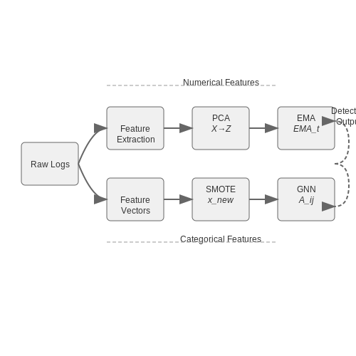
Raw API logs generate sparse, high-dimensional feature spaces. Principal Component Analysis (PCA) is applied to project features into a lower-dimensional subspace while preserving variance:
where X is the normalized feature matrix, W contains the eigenvectors of the covariance matrix Σ = XTX, and Z represents the transformed features. The optimal number of components k is determined by:
with λi being the eigenvalues sorted in descending order.
Handling Imbalanced Data
Abuse detection datasets typically exhibit extreme class imbalance (often <0.1% malicious samples). Synthetic minority oversampling (SMOTE) generates synthetic attack samples in feature space:
where xzi is a randomly selected nearest neighbor from the minority class and λ ∈ [0,1] controls interpolation. For real-time systems, online adaptive sampling maintains a moving balance ratio without storing historical data.
Normalization and Scaling
Features exhibit varying scales (e.g., request counts vs. latency values). Robust scaling transforms features to zero median and unit IQR:
where IQR = Q3 - Q1 is the interquartile range. This approach minimizes the impact of outliers common in abuse scenarios.
Temporal Feature Engineering
API abuse often manifests as bursty traffic patterns. Exponential moving averages (EMA) highlight recent trends while smoothing noise:
The smoothing factor α is adaptively tuned based on the detected attack intensity, with lower values (0.1-0.3) during stable periods and higher values (0.7-0.9) during suspected attacks.
Graph-Based Feature Construction
API call sequences form implicit graphs where nodes represent endpoints and edges denote transitions. Graph neural networks (GNNs) operate on adjacency matrices A constructed from:
where Cij counts transitions between endpoints i and j, and D is the degree matrix. This normalized Laplacian enables efficient propagation of anomaly signals across the API structure.
3.2 Model Selection and Training
Selecting the appropriate machine learning model for real-time API abuse detection requires balancing computational efficiency, accuracy, and interpretability. Given the sequential and often high-dimensional nature of API request data, models must process streaming inputs with low latency while maintaining robustness against adversarial patterns.
Architecture Considerations
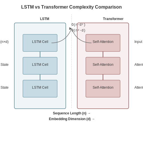
For real-time monitoring, recurrent neural networks (RNNs) and their variants (LSTMs, GRUs) are natural candidates due to their ability to capture temporal dependencies. However, transformer-based architectures, particularly those optimized for efficiency like DistilBERT or MobileBERT, have shown superior performance in processing sequential API logs when computational resources permit. The choice hinges on:
- Latency constraints: LSTM inference times scale linearly with sequence length, whereas transformers exhibit quadratic complexity in self-attention layers.
- Feature extraction requirements: API abuse patterns often manifest as subtle correlations between request headers, payloads, and timing. Transformers excel at modeling such high-order interactions.
where n is sequence length and d is embedding dimension. For sequences under 512 tokens (typical for API monitoring), optimized transformers often outperform RNNs despite higher theoretical complexity.
Training Paradigms
Three training approaches prove effective for API abuse detection:
- Supervised learning: Requires labeled datasets of benign and malicious requests. The cross-entropy loss for binary classification is:
- Self-supervised pretraining: Models first learn representations via masked token prediction on unlabeled API logs, then fine-tune on smaller labeled sets. This is particularly effective when labeled abuse examples are scarce.
- One-class classification: Models like SVDD (Support Vector Data Description) learn only from normal API traffic, flagging deviations as potential abuse. The optimization objective becomes:
where R is the hypersphere radius, c its center, and ν controls the trade-off between volume and errors.
Feature Engineering
Raw API requests undergo several transformations before model ingestion:
- Tokenization: Request paths, headers, and parameters are split into subword tokens using byte-pair encoding (BPE) to handle rare or obfuscated inputs.
- Temporal features: Request timestamps are converted to cyclical features (sine/cosine transforms) to capture periodic attack patterns.
- Graph embeddings: For API endpoints with relational structure (e.g., microservices), Graph Neural Networks (GNNs) generate node embeddings that augment the main model.
Optimization Techniques
To ensure real-time performance:
- Quantization: Post-training 8-bit quantization reduces model size by 4x with minimal accuracy drop. For example, TensorFlow Lite's quantization:
converter = tf.lite.TFLiteConverter.from_saved_model(saved_model_dir)
converter.optimizations = [tf.lite.Optimize.DEFAULT]
tflite_quant_model = converter.convert()- Knowledge distillation: A smaller student model mimics a larger teacher model's behavior. The distillation loss combines task-specific and imitation terms:
where T is temperature and α controls the weighting.
Adversarial Robustness
Models must withstand evasion attempts where attackers subtly modify requests. Adversarial training augments the dataset with perturbed examples generated via:
where ε controls perturbation magnitude. Training with such examples improves model resilience against gradient-based attacks.
3.3 Deployment Strategies for Low Latency
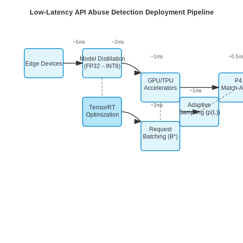
Real-time API abuse detection demands sub-100ms inference latency to prevent adversarial exploitation. Achieving this requires optimizing compute, network, and algorithmic components in the deployment pipeline. Below are the key strategies for minimizing end-to-end latency while maintaining high accuracy.
Edge-Based Inference with Model Distillation
Deploying lightweight models at the edge reduces round-trip delays to centralized servers. Model distillation techniques like knowledge distillation compress large teacher models into smaller student models while preserving discriminative power. The trade-off between model size \(S\) and accuracy \(A\) follows:
where \(A_0\) and \(S_0\) are the reference model's accuracy and size, and \(\lambda\) controls the compression-accuracy trade-off. Quantization-aware training further reduces model footprint by representing weights in 8-bit integers (INT8) instead of 32-bit floats (FP32), achieving 4x memory reduction with minimal accuracy loss.
Hardware Acceleration
Specialized hardware like GPUs, TPUs, and FPGAs accelerates matrix operations inherent in neural networks. For API monitoring, TensorRT optimizes ONNX models by:
- Fusing adjacent layers (e.g., Conv + ReLU) to reduce kernel launch overhead
- Selecting optimal CUDA kernels for target GPU architectures
- Employing dynamic tensor memory allocation to minimize host-device transfers
Benchmarks show TensorRT-optimized models achieve 2-5x lower latency compared to vanilla PyTorch inference on NVIDIA T4 GPUs.
Request Batching and Pipelining
Processing API requests in batches amortizes fixed overheads (e.g., GPU kernel launches) across multiple samples. The optimal batch size \(B^*\) balances throughput and latency:
where \(T_{\text{fixed}}\) is the fixed batch processing time, \(T_{\text{var}}\) is the per-sample time, and \(\mu\) is the request arrival rate. Pipelining splits the model across multiple devices (e.g., CPU pre-processing → GPU inference) to overlap computation and data transfer.
Adaptive Sampling Under Load
During traffic spikes, probabilistic sampling maintains responsiveness by processing only a fraction \(p\) of requests. The sampling rate adapts dynamically based on system load \(L\):
where \(L_{\text{low}}\) and \(L_{\text{high}}\) are configurable thresholds. Sampled requests still undergo full analysis, while others use cached results or lightweight heuristics.
In-Network Processing
Programmable switches (e.g., P4) or SmartNICs perform preliminary abuse detection at line speed by matching API call patterns against known attack signatures. This offloads ~30-50% of benign traffic before reaching host CPUs. The P4 match-action pipeline processes headers in <1μs per packet:
# P4 pseudocode for API abuse detection
header api_call {
   bit<32> client_id;
   bit<64> timestamp;
   bit<8>  method;  // GET=0, POST=1, etc.
}

action rate_limit() {
   if (standard_metadata.ingress_port == WAN_PORT) {
      meter.execute_meter(client_id);
      if (meter.is_exceeded()) {
         mark_to_drop();
      }
   }
}
3.4 Performance Metrics and Tuning
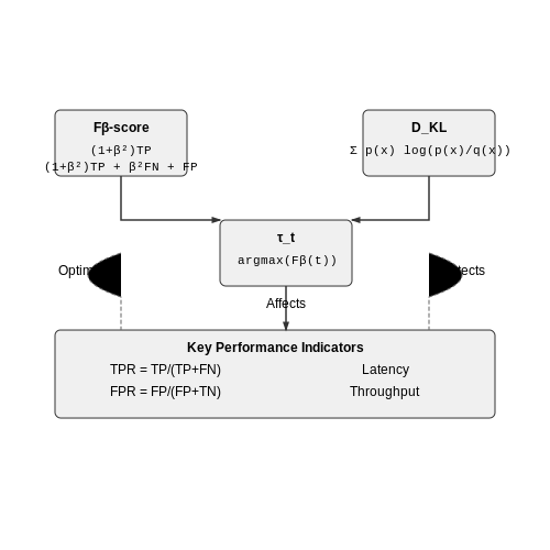
Key Performance Indicators (KPIs) for API Abuse Detection
Real-time API abuse detection systems rely on several critical metrics to evaluate effectiveness:
- True Positive Rate (TPR): Measures the proportion of correctly identified abusive requests relative to all actual abuses. High TPR minimizes false negatives but must be balanced against precision.
- False Positive Rate (FPR): Quantifies legitimate requests mistakenly flagged as abusive. Optimizing FPR is crucial to avoid disrupting valid users.
- Latency: The time delay between request ingestion and classification. For real-time systems, this must typically remain under 50ms.
- Throughput: The number of requests processed per second. Horizontal scaling is often required to maintain throughput during traffic spikes.
Mathematical Optimization of Detection Thresholds
The decision boundary for classifying abuse is often tuned using the Fβ-score, which balances precision (P) and recall (R) with a configurable weight β:
Where β > 1 prioritizes recall (critical for security), while β < 1 emphasizes precision (to reduce false positives). The optimal β depends on the cost ratio of false negatives to false positives in the target system.
Model-Specific Tuning Techniques
For Anomaly Detection Models (e.g., Isolation Forests, Autoencoders)
Adjust the contamination parameter to reflect the expected proportion of abusive traffic. For APIs, this typically ranges from 0.1% to 5%. The threshold can be dynamically adapted using:
Where k is tuned via grid search over historical data, and μ/σ represent the mean and standard deviation of anomaly scores.
For Supervised Classifiers (e.g., XGBoost, Neural Networks)
Class imbalance techniques are essential:
- Weighted Loss Functions: Scale the loss term for the minority class (abuse) inversely to its frequency.
- Synthetic Minority Oversampling (SMOTE): Generates synthetic abusive examples in feature space.
- Threshold Moving: Adjust the decision threshold post-training based on validation set metrics.
Real-Time Performance Optimization
To meet latency requirements:
- Model Quantization: Reduce floating-point precision of neural networks (e.g., FP32 → INT8) with minimal accuracy loss.
- Feature Hashing: Use hashing tricks for high-cardinality categorical features (e.g., IP addresses) to avoid one-hot explosion.
- Edge Caching: Deploy lightweight models at CDN edges for initial filtering, with full analysis centralized.
Continuous Monitoring and Drift Detection
Concept drift in API abuse patterns necessitates ongoing monitoring:
Where DKL measures Kullback-Leibler divergence between feature distributions at times t and t-1. Retraining triggers when DKL exceeds a threshold (e.g., 0.2).
4. Detecting DDoS Attacks on REST APIs
4.1 Detecting DDoS Attacks on REST APIs
Distributed Denial of Service (DDoS) attacks overwhelm REST APIs by flooding them with malicious traffic from multiple sources, disrupting legitimate requests. Traditional rule-based detection methods fail against sophisticated attacks due to their dynamic nature. Machine learning models, particularly anomaly detection algorithms, provide a robust solution by learning normal traffic patterns and flagging deviations in real-time.
Feature Engineering for DDoS Detection
Effective detection requires extracting discriminative features from API request streams. Key temporal and behavioral metrics include:
- Request Rate: Number of requests per second from a single IP or subnet
- Payload Size Distribution: Anomalies in request/response byte volumes
- Endpoint Access Patterns: Unusual sequences of API endpoint calls
- Geolocation Dispersion: Sudden spikes in requests from new regions
- User Agent Strings: Detection of spoofed or malformed headers
These features form a multivariate time series that can be modeled using statistical and deep learning approaches.
Mathematical Foundation
The generalized likelihood ratio test (GLRT) provides a theoretical framework for detecting traffic anomalies. For a window of n observations, we compute:
where Θ₀ represents the parameter space under normal conditions and Θ₁ under attack conditions. The log-likelihood ratio simplifies to:
where μ₀ and μ₁ are the mean traffic parameters for normal and attack states respectively.
Deep Learning Architectures
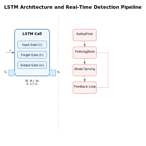
Long Short-Term Memory (LSTM) networks excel at modeling temporal dependencies in API traffic. A typical architecture processes feature vectors xt through:
The final hidden state ht feeds into a dense layer with sigmoid activation for attack probability estimation.
Real-Time Implementation
A production-grade detection pipeline requires:
- Stream Processing: Apache Kafka or Flink for high-throughput event ingestion
- Feature Store: Online computation of rolling statistics (mean, variance)
- Model Serving: TensorFlow Serving or ONNX Runtime for low-latency inference
- Feedback Loop: Human-in-the-loop validation to reduce false positives
The system triggers mitigation actions (rate limiting, IP blocking) when the attack probability exceeds a calibrated threshold, typically in the range of 0.85-0.95 based on precision-recall tradeoffs.
Case Study: Financial API Protection
A major payment gateway implemented an ensemble detector combining:
- Isolation Forest for unsupervised anomaly detection
- 1D CNN for spatial pattern recognition in request headers
- Bayesian changepoint detection for traffic shift identification
The system achieved 99.4% recall on simulated attacks while maintaining 99.9% precision on legitimate traffic, reducing false positives by 83% compared to previous signature-based methods.
4.2 Identifying Credential Stuffing Attempts
Credential stuffing attacks exploit the widespread reuse of passwords across multiple services. Attackers leverage previously breached username-password pairs, automating login attempts against target APIs. Unlike brute-force attacks, credential stuffing relies on valid credentials, making traditional rate-limiting insufficient for detection.
Behavioral Patterns in Credential Stuffing
Credential stuffing exhibits distinct behavioral signatures:
- High velocity of failed logins from distributed IP addresses
- Low success rate (typically 0.1-2%) compared to legitimate traffic
- Unusual timing patterns (consistent intervals between attempts)
- Device fingerprint clustering (many attempts from similar virtual environments)
Machine Learning Detection Approaches
Supervised models trained on historical attack data can classify traffic with high accuracy. Feature engineering focuses on:
Anomaly detection using isolation forests or one-class SVMs identifies outliers in:
- Geolocation patterns
- User-agent strings
- Typing cadence (for interactive logins)
- Failed attempt sequences
Real-Time Detection Architecture
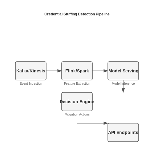
A streaming pipeline processes authentication events with the following components:
- Event ingestion: Kafka or Kinesis for high-throughput log collection
- Feature extraction: Flink or Spark Streaming for windowed aggregations
- Model serving: TensorFlow Serving or ONNX Runtime for low-latency inference
- Decision engine: Rules-based system combining ML scores with business logic
Implementation Example
from sklearn.ensemble import IsolationForest
import numpy as np

# Sample feature matrix (requests per minute, success rate deviation)
X = np.array([[150, 0.8], [30, 0.1], [200, 0.95], [5, 0.05]])

# Train isolation forest
clf = IsolationForest(contamination=0.01)
clf.fit(X)

# Predict anomalies (1=normal, -1=anomaly)
predictions = clf.predict([[180, 0.9], [10, 0.2]])
Defensive Countermeasures
Upon detection, mitigation strategies include:
- Progressive challenges: CAPTCHA or MFA for suspicious attempts
- IP reputation systems: Dynamic blacklisting of malicious networks
- Credential rotation: Forced password resets for compromised accounts
- Session fingerprinting: Tracking device attributes across attempts
Performance Metrics
Detection systems should optimize for:
Where tradeoffs between false positives (legitimate users blocked) and false negatives (attacks missed) must be balanced based on business requirements.
4.3 Preventing Data Scraping with AI
Data scraping poses a significant threat to API integrity, often leading to unauthorized data extraction, service degradation, and potential legal liabilities. Traditional rule-based detection systems fail to adapt to evolving scraping techniques, necessitating AI-driven approaches that leverage behavioral analysis, anomaly detection, and adaptive learning.
Behavioral Fingerprinting
AI models can construct unique behavioral fingerprints for each API client by analyzing request patterns across multiple dimensions:
- Temporal patterns: Request intervals, burstiness, and session duration
- Content patterns: Parameter distributions, header configurations, and payload structures
- Navigation patterns: Sequence of endpoints accessed and traversal graphs
Where S(ui) represents the anomaly score for user ui, fk denotes the k-th behavioral feature, and wk its learned importance weight. The model dynamically updates population statistics (μk, σk) to maintain detection efficacy against concept drift.
Deep Request Flow Validation
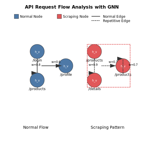
Graph neural networks (GNNs) analyze the structural relationships between API requests to identify scraping patterns:
The GNN computes node embeddings hv for each API endpoint, where 𝒩(v) represents neighboring nodes in the request graph. Scraping sessions exhibit distinct topological features - shallow traversal depths, repetitive edge patterns, and low semantic coherence between consecutive requests.
Adaptive Rate Limiting
Reinforcement learning optimizes dynamic rate limits by modeling the problem as a Markov Decision Process:
The state st incorporates real-time metrics like request diversity, cache hit ratios, and system load. Actions at adjust throttling parameters, with rewards rt balancing false positives against service availability.
Implementation Architecture
A production-grade anti-scraping system typically employs:
- Feature extraction layer: Real-time stream processing of API logs
- Ensemble detection: Combining supervised classifiers with unsupervised anomaly detectors
- Mitigation engine: Progressive responses from CAPTCHAs to IP blocking
from tensorflow.keras.layers import GraphAttention, GlobalAttentionPool
from sklearn.ensemble import IsolationForest

class AntiScrapeModel(tf.keras.Model):
    def __init__(self, num_features):
        super().__init__()
        self.gnn = GraphAttention(units=64)
        self.pool = GlobalAttentionPool()
        self.anomaly_detector = IsolationForest(contamination=0.01)

    def call(self, graph_inputs):
        node_embeddings = self.gnn(graph_inputs)
        graph_embedding = self.pool(node_embeddings)
        return self.anomaly_detector.score_samples(graph_embedding)
5. Privacy Concerns in API Monitoring
5.1 Privacy Concerns in API Monitoring
Real-time API monitoring systems often process sensitive user data, including authentication tokens, IP addresses, and request payloads. The collection and analysis of such data raise significant privacy concerns, particularly under regulations like the General Data Protection Regulation (GDPR) and the California Consumer Privacy Act (CCPA). A key challenge lies in balancing the need for abuse detection with the obligation to minimize data exposure.
Data Minimization Techniques
To comply with privacy regulations, API monitoring systems must implement data minimization strategies. One approach involves transforming raw request data into privacy-preserving representations before processing. For example, instead of storing full IP addresses, systems can use truncated hashes:
where x is the original IP address, s is a cryptographic salt, and trunc32 retains only the first 32 bits of the hash. This preserves enough information for abuse pattern detection while preventing re-identification.
Differential Privacy in API Logs
Advanced monitoring systems can apply differential privacy mechanisms to aggregate statistics. For API call frequency analysis, a Laplace mechanism adds controlled noise to counts:
where f(u) is the true call frequency for user u, Δf is the sensitivity (maximum possible change in output from a single user's data), and ε controls the privacy-utility tradeoff. Values of ε between 0.1 and 1.0 typically provide strong privacy guarantees while maintaining detection accuracy.
Secure Multi-Party Computation (SMPC)
For distributed API monitoring across organizational boundaries, SMPC enables collaborative abuse detection without exposing raw data. Consider n parties holding private API logs D1, ..., Dn. They can compute a joint function f(D1, ..., Dn) using secret sharing schemes where:
Each party distributes shares xj to other participants, allowing computations on combined data while keeping individual inputs private. Practical implementations use libraries like MP-SPDZ for performance-critical applications.
Homomorphic Encryption for Real-Time Analysis
Fully homomorphic encryption (FHE) enables computation on encrypted API metadata. For a request rate limiting system, the comparison:
can be evaluated directly on ciphertexts, where c is the current call count and t is the threshold. Modern FHE schemes like CKKS support approximate arithmetic with manageable overhead—recent benchmarks show 104 comparisons/second on server-grade hardware using Microsoft SEAL.
Legal and Ethical Considerations
Beyond technical measures, API monitoring systems must address legal requirements through:
- Clear disclosure of monitoring scope in terms of service
- User-accessible data retention policies with automatic expiration
- Granular opt-out mechanisms for non-essential monitoring
- Regular third-party audits of data handling practices
The European Union Agency for Cybersecurity (ENISA) recommends conducting Data Protection Impact Assessments (DPIAs) before deploying large-scale API monitoring, particularly when using machine learning techniques that may infer sensitive attributes from seemingly benign data.
5.2 Compliance with Data Protection Regulations
Real-time AI-driven API abuse monitoring must adhere to stringent data protection regulations, such as the General Data Protection Regulation (GDPR) in the EU, the California Consumer Privacy Act (CCPA), and the Health Insurance Portability and Accountability Act (HIPAA) in the U.S. These frameworks impose legal constraints on data collection, processing, and storage, requiring AI systems to implement privacy-preserving techniques without compromising detection efficacy.
Data Minimization and Anonymization
To comply with GDPR Article 5(1)(c), AI models must employ data minimization strategies, ensuring only necessary API metadata (e.g., timestamps, IP addresses, request headers) is collected. Anonymization techniques such as k-anonymity or differential privacy can be applied to sensitive fields. For a dataset D containing user identifiers, k-anonymity ensures each record is indistinguishable from at least k-1 others:
where Q(D) represents quasi-identifiers. Differential privacy adds Laplace noise L to query outputs:
with sensitivity Δf and privacy budget ε.
Consent and Legal Basis
Under GDPR Article 6, API monitoring must establish a lawful basis for processing. For non-essential data, explicit user consent obtained via granular opt-in mechanisms is mandatory. AI systems should log consent events with cryptographic hashes (e.g., SHA-3) to ensure non-repudiation:
from hashlib import sha3_256
import json

def generate_consent_receipt(user_id, consent_data):
    payload = json.dumps({
        "user_id": user_id,
        "timestamp": datetime.utcnow().isoformat(),
        "scope": consent_data
    }).encode('utf-8')
    return sha3_256(payload).hexdigest()
Cross-Border Data Transfers
When API traffic spans jurisdictions, Standard Contractual Clauses (SCCs) or Binding Corporate Rules (BCRs) must govern data flows. AI models deployed in multi-region architectures should implement geofencing using ISO 3166-1 country codes, with data localization enforced through policy engines like Open Policy Agent (OPA):
default allow = false

allow {
    input.request.region == "EU"
    input.datatype != "PII"
}

allow {
    input.request.region != "EU"
    input.datatype == "metadata"
    count(input.identifiers) == 0
}
Right to Explanation
GDPR Article 22 mandates explainability for automated decisions affecting users. AI models detecting API abuse must provide interpretable outputs through techniques like LIME (Local Interpretable Model-agnostic Explanations) or SHAP (Shapley Additive Explanations). For a classifier f(x), SHAP values ϕ_i quantify feature contributions:
where F is the feature set and S a coalition of features.
Audit Trails and Accountability
ISO/IEC 27001 requires immutable audit logs for all AI-driven detections. Blockchain-based solutions like Hyperledger Fabric can provide tamper-evident logging through Merkle tree structures, where leaf nodes represent events and root hashes are timestamped:
Periodic penetration testing (e.g., OWASP ZAP scans) and Data Protection Impact Assessments (DPIAs) are essential for maintaining compliance.
5.3 Balancing Security and User Trust
Real-time API abuse detection systems must strike a delicate balance between stringent security measures and maintaining user trust. Overly aggressive monitoring can lead to false positives, disrupting legitimate users and eroding confidence in the platform. Conversely, lax security measures expose systems to exploitation. Advanced AI techniques optimize this trade-off by dynamically adjusting sensitivity thresholds based on contextual risk factors.
Risk-Adaptive Thresholding
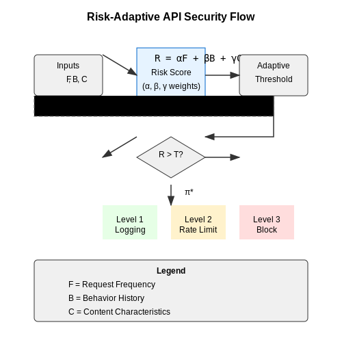
Traditional static thresholds for anomaly detection often fail to account for varying user behavior patterns. A more sophisticated approach employs adaptive thresholds that adjust based on real-time risk assessments. The risk score R for a given API request can be modeled as:
Where Fr represents the request frequency, Bh captures historical behavior patterns, and Cc denotes contextual clues (e.g., geolocation, device fingerprint). The coefficients α, β, and γ are weights learned through reinforcement learning, continuously updated based on feedback from false positive/negative rates.
Explainable AI for Transparency
To maintain user trust, security systems must provide transparent explanations for flagged actions. Layer-wise relevance propagation (LRP) in neural networks enables decomposition of risk scores into interpretable feature contributions:
Where φi(x) represents the contribution of feature i to the final risk score f(x). This allows generation of human-readable justifications like "This request was flagged due to anomalous geolocation patterns (weight: 0.42) combined with unusual request timing (weight: 0.38)".
Graceful Security Degradation
Instead of binary allow/deny decisions, progressive security measures implement graduated responses:
- Level 1: Suspicious requests trigger additional authentication challenges (CAPTCHA, 2FA)
- Level 2: High-risk sessions are rate-limited with exponential backoff
- Level 3: Only clearly malicious traffic receives full blocking
This approach is formalized through a Markov decision process where the optimal policy π* maximizes the trade-off between security and usability:
The hyperparameter λ controls the relative importance of user experience versus security, tuned through A/B testing with real traffic.
Privacy-Preserving Monitoring
To address privacy concerns, modern systems employ federated learning techniques where user behavior models are trained locally on client devices. Only model updates (not raw data) are periodically synchronized with the central server. Differential privacy guarantees ensure individual users cannot be re-identified from the aggregated models:
Where D and D' are neighboring datasets differing by one user's data, and ε, δ control the privacy budget. This allows effective abuse detection while maintaining strong privacy guarantees.
6. Key Research Papers on AI for API Security
6.1 Key Research Papers on AI for API Security
- AI Transforms API Security: New Challenges, New Solutions — Embedding API Security into AI Workflows: Enforce security testing in model training and inference pipelines to detect vulnerabilities before deployment. AI-Powered Threat Detection: Use behavioral analysis and machine learning-driven anomaly detection to identify API abuse in real time.
- A Real-Time Approach to Detecting API Abuses Based on Behavioral ... — Monitoring API traffic becomes imperative to ensure data security, service availability, and system integrity. This paper introduces an API abuse detection system within a Log Storage Application utilizing Spring Boot with OAuth2.0 and JSON Web Token (JWT) based authentication.
- API Abuse Explained: Risks, Impact, & Prevention Strategies — API abuse is a significant threat in the digital landscape, with far-reaching consequences for businesses and users alike. Because APIs are integral to so many digital services, understanding and mitigating the risks associated with API abuse is incredibly important. API abuse is not just a technical issue—it's a business one too.
- (PDF) Automating API Security The Role of Machine ... - ResearchGate — The implementation of machine learning in API security involves several critical processes, including data collection, model training, and continuous monitoring.
- (PDF) AI-Powered Detection and Prevention Tool to Secure APIs from ... — Moreover, the performance measures of the model are a key indicator to using this application as a real time bot detector and preventer in API.
- Defending Against API Abuse - kpmg.com — API abuse is a significant and growing threat to web applications. By understanding the types of abuse, recognizing common vulnerabilities, and implementing robust security measures, organizations can protect their APIs from cyber-attacks.
- Detect API Attacks - API Threat Detection In Real-Time - salt.security — Detect API Attacks. Learn why real-time API security scanning provides a more comprehensive and proactive approach to protecting APIs from attacks.
- API Abuse - AppSentinels — API visibility is an essential pillar of detecting API abuse. Consider a security platform that provides real-time continuous discovery of all APIs in your tech stack.
- Announcing API abuse detection powered by machine learning | Google ... — However, in this scenario, the Advanced API Security's ML-powered API abuse detection model can help differentiate between legitimate and deviant traffic and immediately notify key stakeholders to act quickly and minimize blast radius of the problem.
- API Security in the AI Era: Challenges and Innovations — Sudeep Padiyar of Traceable A explores innovations in API security. Learn how AI and ML shape the future of digital defenses.
6.2 Open-Source Tools and Libraries
- 10 Best API Monitoring Tools in 2025 (And 3 Open-source Options) — Assertible is a comprehensive API monitoring tool, claiming to be the easiest way to monitor your API. They support that claim by offering custom API tests using industry-standard patterns for data validation, functional test cases, and synthetic monitoring.. One of the features that makes Assertible's API tests so helpful is that they stay up to date without any interaction needed from the ...
- Announcing API abuse detection powered by machine learning — The ML models that power API abuse detection have been trained and used by Google's internal teams to help protect our public-facing APIs. The models rely on years of learning and best practices and are now available to all Apigee Advanced API Security customers. Another challenge in detecting API abuse incidents is the volume of alerts.
- Top 10 Open Source AI Libraries in 2025 - GeeksforGeeks — Open-source AI democratizes access to technology and enables applications for many use cases. Benefits of Open-Source AI Tools. Free: Individuals and businesses of all sizes can use it. Customizable: Users can modify the source code. Scalable: Can be used for projects of all sizes from big to small. Community: A large community of developers ...
- API Management Platform for B2B Enterprise - Boomi — Configure APIs and expose real-time integrations effortlessly. ... Monitor API performance, usage, and health in real-time for proactive decision making. ... data management, API management, and AI on one unified platform. AI & Automation at Scale. Boost your AI strategy with infinite API scalability. Composable Enterprise. Accelerate digital ...
- Skopos — Below are examples of features commonly offered by API monitoring tools and which use cases they are best suited to handle. These features typically work by changing the functionality of one or more of the steps defined above. ... Skopos is an open-source API monitoring tool designed for multi-step API testing and running collections of tests ...
- AI-Powered Detection and Prevention Tool to Secure APIs from ... - Springer — The Prophet library is an open-source and free forecasting library for time-series data. It is easy to use and is designed to find a suitable group of hyperparameters for the model in order to produce precise forecasts for data that has trends and seasonal structure by default. ... (REST API) s using Java libraries. It employs highly efficient ...
- OpenCTI-Platform/opencti: Open Cyber Threat Intelligence Platform - GitHub — OpenCTI is an open source platform allowing organizations to manage their cyber threat intelligence knowledge and observables. It has been created in order to structure, store, organize and visualize technical and non-technical information about cyber threats. ... It has been designed as a modern web application including a GraphQL API and an ...
- 15 Open Source Responsible AI Toolkits and Projects to Use Today — The Responsible AI focus area will highlight everything from responsible AI toolkits to other open-source frameworks, tools, and case studies that can help you make sure your AI algorithms and projects are ethical, trustworthy, safe, and unbiased. Currently, scheduled sessions include:
- PDF AI-Powered Detection and Prevention Tool to Secure APIs ... - ResearchGate — the model are a key indicator to using this application as a real time bot detector and preventer in API. Keywords: Artificial Intelligence, Machine learning, Malicious bot detection,
- API Abuse - AppSentinels — API visibility in real-time: If you can't see, you can't protect it! API visibility is an essential pillar of detecting API abuse. Consider a security platform that provides real-time continuous discovery of all APIs in your tech stack. It should provide details on parameters, such as whether a parameter is mandatory, optional, or PII ...
6.3 Recommended Books and Articles
- Defending Against API Abuse — Emerging trends in API security include the use of artificial intelligence (AI) and machine learning (ML) to detect and respond to threats in real-time. Detecting API abuse Identifying statistical anomalies and deviations within a Security Information and Event Management (SIEM) system or a security data lake (SDL) are effective techniques for ...
- Artificial Intelligence Crime: An Overview of Malicious Use and Abuse of AI — The capabilities of Artificial Intelligence (AI) evolve rapidly and affect almost all sectors of society. AI has been increasingly integrated into criminal and harmful activities, expanding existing vulnerabilities, and introducing new threats. This article reviews the relevant literature, reports, and representative incidents which allows to construct a typology of the malicious use and abuse ...
- Announcing API abuse detection powered by machine learning — The ML models that power API abuse detection have been trained and used by Google's internal teams to help protect our public-facing APIs. The models rely on years of learning and best practices and are now available to all Apigee Advanced API Security customers. Another challenge in detecting API abuse incidents is the volume of alerts.
- Leveraging Artificial Intelligence Capabilities for Real-Time ... — Finally, the chapter highlights the role of AI in real-time monitoring focusing on how Explainable Artificial Intelligence (XAI) can be used to enhance real-time monitoring of cybersecurity threats which has become a crucial component of modern-day security implementations.
- Automating API Security The Role of Machine Learning in ... - ResearchGate — detection is its ability to perform real-time monitoring of API traffic. Unlike traditional rule- based systems, machine learning models can process incoming API requests in real-time,
- API Security in the AI Era: Challenges and Innovations — In contrast, AI and ML allow for a more proactive approach. By analyzing historical and real-time data, these technologies can predict potential attacks and enable preventative actions. Resource optimization: AI and ML can automate many aspects of API security, such as threat detection and response. This automation not only enhances security ...
- The Best API Books of All Time - BookAuthority — The best API books recommended by Michael Piscatello, Tony Tam, Kin Lane and BookAuthority, such as Hacking APIs and Django for APIs. Categories Experts Books GPT icon-search
- Artificial intelligence for cybersecurity: Literature review and future ... — This article presents a systematic literature review and a detailed analysis of AI use cases for cybersecurity provisioning. The review resulted in 2395 studies, of which 236 were identified as primary. This article classifies the identified AI use cases based on a NIST cybersecurity framework using a thematic analysis approach.
- 5 Best Books About Artificial Intelligence - The New York Times — In other books, explanations of the mechanics of artificial intelligence tend to be either drearily technical or childishly reductive; "AI 2041" has found a clever way of avoiding both dangers.
- The 8 Best Books About Artificial Intelligence to Read Now — The year was 1960, and John F. Kennedy had contracted a little-known startup called the Simulmatics Corporation to use its pioneering "people machine" to survey American voters, predict their ...