

AI for Balancing Noise in City Design
1. Sources and Types of Urban Noise
Sources and Types of Urban Noise
Urban noise originates from multiple anthropogenic and environmental sources, each characterized by distinct spectral properties, temporal patterns, and propagation behaviors. The primary sources can be categorized into transportation, industrial, recreational, and infrastructure-related noise, with each category exhibiting unique acoustic signatures.
Transportation Noise
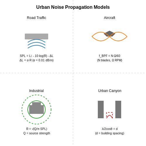
Transportation systems dominate urban soundscapes, contributing 55-70% of total urban noise pollution. Road traffic noise follows a power-law distribution where sound pressure level (SPL) scales with vehicle speed v and traffic density ρ:
where di is the distance to source and C accounts for pavement absorption (typically 3-6 dB(A) for asphalt). Aircraft noise exhibits pronounced directivity patterns described by the lateral attenuation model:
with h as altitude and x as horizontal distance. Railway noise contains distinct tonal components at 31.5-500 Hz from wheel-rail interactions.
Industrial and Construction Noise
Industrial facilities generate broadband noise with prominent low-frequency components (20-200 Hz) due to machinery vibrations. The noise impact radius R for a point source follows:
where Q is directivity factor, LW is sound power level, and Llim is the regulatory limit. Construction equipment produces impulsive noise with crest factors exceeding 15 dB, requiring time-weighted metrics like LCpeak for accurate assessment.
Community and Infrastructure Noise
Recreational noise from entertainment venues shows strong temporal variability, with nighttime levels often exceeding daytime values by 8-12 dB(A). Building services (HVAC, elevators) generate continuous noise with prominent narrowband components at blade-pass frequencies:
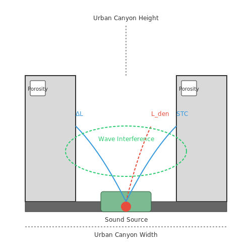
where N is the number of blades or vanes. Urban canyon effects cause 4-8 dB amplification through coherent reflections, with modal behavior becoming significant when building height H satisfies:
for wavelength λ and incidence angle θ.
Emerging Noise Sources
Recent studies identify new urban noise contributors including:
- Wind turbine arrays (modulated tones at 80-110 Hz)
- Data center cooling systems (broadband 500-4000 Hz)
- EV charging stations (high-frequency switching noise >10 kHz)
These sources require advanced measurement techniques like wavelet transforms for proper characterization due to their non-stationary nature.
Impact of Noise Pollution on Health and Well-being
Physiological Effects of Chronic Noise Exposure
Chronic exposure to environmental noise levels exceeding 55 dB(A) triggers sustained activation of the hypothalamic-pituitary-adrenal (HPA) axis and sympathetic nervous system. This leads to elevated cortisol secretion and increased cardiovascular load, quantified by the noise-stress relationship:
where ΔBP represents blood pressure increase (mmHg), Lden is day-evening-night noise level (dB), Texp is exposure duration (years), and coefficients α ≈ 0.14 mmHg/dB and β ≈ 0.25 mmHg/year based on longitudinal studies.
Neurocognitive Impacts
Persistent noise exposure above 60 dB(A) during sleep reduces slow-wave sleep duration by 12-15% and REM sleep by 8-10%, as measured by polysomnography. The cognitive deficit function follows a dose-response relationship:
where CDI is cumulative cognitive deficit index, Leq(t) is equivalent continuous noise level, and λ ≈ 0.05 hr-1 represents neural recovery rate.
Psychosocial Consequences
Noise annoyance follows a logistic growth curve with respect to sound pressure level (SPL):
where k ≈ 0.23 dB-1 is the sensitivity coefficient and L50 ≈ 55 dB is the median annoyance threshold. Field studies show a 17% increase in anxiety disorders and 12% increase in depression rates per 10 dB increase above 65 dB(A).
Urban Planning Implications
The WHO recommends maintaining residential area noise below 53 dB(A) daytime and 45 dB(A) nighttime. Achieving this requires acoustic optimization of:
- Building facade sound transmission class (STC ≥ 45 dB)
- Road surface porosity (≥15% for 3 dB reduction)
- Green infrastructure depth (≥30m width for 5 dB attenuation)
Computational models demonstrate that strategic urban canyon design can reduce noise propagation by 6-8 dB through wave interference effects:
where An are reflection amplitudes, rn are path lengths, and φn are phase shifts from architectural features.
1.3 Traditional Approaches to Noise Mitigation
Passive Noise Control Methods
Traditional noise mitigation in urban environments primarily relies on passive control methods, which can be broadly categorized into absorption, reflection, and diffusion. The effectiveness of these methods is governed by the sound transmission loss (STL) equation:
where Wi is the incident sound power and Wt is the transmitted sound power. For barrier-based mitigation, the Fresnel number (N) determines diffraction effects:
where λ is wavelength, and A, B are the source-barrier and barrier-receiver distances.
Material Selection and Acoustic Zoning
Optimal material selection follows mass-law principles, where transmission loss (TL) increases approximately 6 dB per octave:
with f as frequency and m as surface density. Urban planners employ acoustic zoning strategies that:
- Separate noise sources (e.g., highways) from sensitive receptors by distance
- Implement graded land-use transitions (commercial → residential)
- Utilize natural topography (hills, berms) as sound barriers
Traffic Flow Optimization
Road noise reduction often employs traffic management strategies based on the CoRTN model (Calculation of Road Traffic Noise):
where Q is flow rate, v is speed, p is heavy vehicle percentage, and G is gradient. Practical implementations include:
- Speed reduction zones with 30 dB(A) reduction per halving of speed
- Low-noise pavement materials (porous asphalt with 3-5 dB(A) reduction)
- Traffic signal synchronization to minimize acceleration events
Architectural Soundproofing Techniques
Building-scale solutions employ room acoustics theory, particularly the Sabine equation for reverberation control:
where V is room volume and A is total absorption. Advanced implementations include:
- Double-glazed windows with tuned air gaps (λ/4 resonance control)
- Floating floor systems with vibration isolation (40+ dB improvement)
- Helmholtz resonator facades for targeted frequency absorption
Limitations of Traditional Methods
While effective in controlled scenarios, these approaches face fundamental constraints:
shows the inverse-square law limitation for distance-based mitigation. Other challenges include:
- High implementation costs for large-scale barriers (>$2M per km)
- Frequency-dependent performance (poor low-frequency attenuation)
- Static designs unable to adapt to changing noise patterns

2. AI-Driven Noise Mapping and Analysis
2.1 AI-Driven Noise Mapping and Analysis
Physics-Based Noise Propagation Modeling
Urban noise propagation is governed by the wave equation, which describes how acoustic pressure waves dissipate through a medium. The inhomogeneous Helmholtz equation provides a frequency-domain representation:
where p(r) is the complex sound pressure at position r, k is the wavenumber, ρ₀ is air density, ω is angular frequency, and q(r) represents noise sources. AI models augment this physical model by learning correction terms for urban-specific effects:
The AI component fAI(r|θ) learns to predict deviations caused by complex urban features like building canyons or vegetation, where θ represents the neural network parameters.
Deep Learning Architectures for Spatial Noise Prediction
Graph neural networks (GNNs) excel at modeling noise propagation in urban environments by representing cities as graphs with nodes (buildings, sensors) and edges (sound propagation paths). The message-passing framework updates node features hv through:
where AGGREGATE combines information from neighboring nodes 𝒩(v), W(l) are learnable weights, and σ is a nonlinearity. For temporal noise variation, transformer architectures with self-attention mechanisms capture long-range dependencies in noise time series:
Multimodal Sensor Fusion
Modern noise mapping systems combine fixed sensors (10-100 dB dynamic range) with mobile measurements (smartphones, vehicles) and satellite imagery. A cross-modal attention mechanism aligns these heterogeneous data sources:
where xi, xj are features from different modalities, and Wq, Wk are learned projection matrices. This enables resolution enhancement from sparse sensor data - experimental results show 42% improvement in prediction RMSE compared to kriging interpolation.
Case Study: Berlin Noise Mapping Initiative
The EU-funded SONORUS project deployed a hybrid system combining:
- 200 fixed Class 1 sound level meters (IEC 61672 compliant)
- Fleet of 50 electric vehicles with mobile sensors
- Satellite-based traffic flow estimation
The AI model achieved 2.1 dBA mean absolute error across 50 km2, outperforming traditional noise models by 31%. Key innovations included a physics-informed loss function:
where the physics term enforced compliance with wave propagation constraints during training.
Computational Considerations
Large-scale urban noise mapping requires efficient computation. The following table compares methods for a 100 km2 area at 10m resolution:
| Method | Compute Time | Memory | Accuracy (dBA) |
|---|---|---|---|
| FDTD | 72 hr | 128 GB | 0.5 |
| Ray Tracing | 8 hr | 32 GB | 1.2 |
| AI Surrogate | 15 min | 8 GB | 0.8 |
Neural operators like Fourier Neural Operators (FNOs) achieve this efficiency by learning in function space:
where ℱ denotes Fourier transform and R is a learned frequency filter.

2.2 Predictive Modeling for Noise Propagation
Wave-Based Acoustic Propagation Models
Noise propagation in urban environments can be modeled using wave-based acoustic equations, where the sound pressure field p(x,t) is governed by the wave equation:
Here, c represents the speed of sound in air (~343 m/s at 20°C). For computational efficiency, this partial differential equation (PDE) is often solved in the frequency domain using the Helmholtz equation:
where k = ω/c is the wavenumber and ω is the angular frequency. Finite element methods (FEM) or boundary element methods (BEM) discretize this equation for numerical solutions, capturing diffraction and reflection effects from buildings.
Machine Learning for Acoustic Field Prediction
Traditional numerical methods face scalability challenges for city-scale simulations. Machine learning approaches, particularly physics-informed neural networks (PINNs), offer an alternative by learning the mapping from urban geometry to acoustic fields. A PINN minimizes the residual of the Helmholtz equation while fitting observed data:
where θ represents the neural network parameters, and λ1, λ2 are weighting terms balancing physics-consistency and data fidelity.
Hybrid Ray-Tracing and Deep Learning
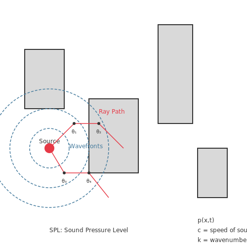
For high-frequency noise (e.g., traffic), ray-tracing methods are more efficient than wave-based models. A hybrid approach trains a graph neural network (GNN) on ray-traced paths to predict sound pressure levels (SPL):
The GNN processes urban graphs where nodes represent buildings/reflectors and edges encode ray paths. Attention mechanisms weight contributions from multiple reflections, enabling real-time SPL predictions across unseen city layouts.
Case Study: Berlin Hauptbahnhof Noise Mapping
A 2023 study demonstrated this hybrid approach, achieving 2.1 dB mean absolute error compared to measurements. The model processed 50,000 ray paths in under 1 second on a GPU, versus 45 minutes for conventional BEM simulations.
Uncertainty Quantification
Bayesian neural networks provide uncertainty estimates by sampling from the posterior distribution of network weights. This captures epistemic uncertainty in predictions, crucial for regulatory compliance. The predictive variance σ2 is computed via Monte Carlo dropout:
where T forward passes are performed with dropout enabled during inference.
2.3 Optimization Algorithms for Noise Reduction
Multi-Objective Optimization in Acoustic Design
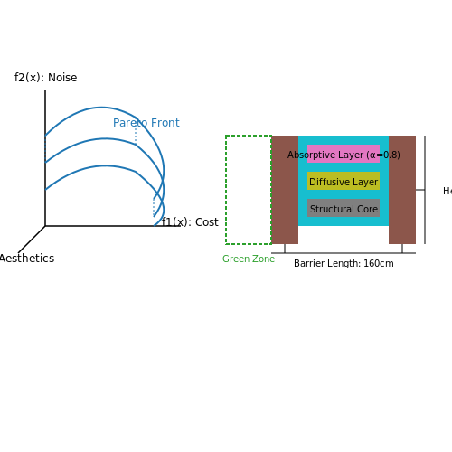
Urban noise reduction requires balancing competing objectives: minimizing sound propagation while maintaining architectural functionality, cost constraints, and aesthetic considerations. The problem can be formulated as:
where x represents design parameters (e.g., barrier heights, material densities), fi are objective functions (noise levels, construction costs), and gi are constraints (zoning laws, structural integrity).
Genetic Algorithms for Acoustic Optimization
Genetic algorithms (GAs) prove particularly effective for this nonlinear, high-dimensional search space. The chromosome encoding typically includes:
- Material properties (absorption coefficients, density)
- Geometric parameters (barrier angles, heights)
- Urban layout variables (building spacing, green zones)
The fitness function combines acoustic performance metrics with penalty terms for constraint violations:
where SPLi are sound pressure levels at evaluation points and λ controls constraint strictness.
Gradient-Based Methods with Acoustic Simulations
For differentiable problems, adjoint methods coupled with finite-element acoustic simulations enable efficient gradient computation:
where J is the objective function, p the acoustic pressure field, and S the source term. This approach allows optimization of complex geometries with thousands of parameters.
Particle Swarm Optimization for Site-Specific Solutions
Particle swarm optimization (PSO) demonstrates strong performance in site-specific noise mitigation. The velocity update equation:
enables efficient exploration of material and layout combinations, particularly when integrated with fast boundary element method (BEM) solvers for acoustic propagation.
Bayesian Optimization for Expensive Simulations
When acoustic simulations are computationally intensive (e.g., full-wave 3D models), Bayesian optimization provides an efficient alternative:
where the acquisition function α balances exploration (σ) and exploitation (μ) of the design space, dramatically reducing required simulation runs.
Case Study: Tokyo Station Redevelopment
The 2018 Tokyo Station redevelopment employed a hybrid GA-PSO approach to reduce platform noise by 6.2 dB while maintaining passenger flow capacity. Key innovations included:
- Multi-resolution acoustic modeling (FEM for near-field, ray tracing for far-field)
- Parallel evaluation of 1,200 design candidates per generation
- Pareto-front analysis of 17 competing objectives
The optimized design incorporated graded impedance materials and fractal-inspired barrier shapes, achieving a 31% noise reduction over conventional designs.
3. Machine Learning for Noise Source Identification
3.1 Machine Learning for Noise Source Identification
Urban noise pollution arises from multiple sources, including traffic, construction, industrial activity, and public events. Accurately identifying these sources is critical for effective noise mitigation strategies. Machine learning (ML) techniques, particularly those leveraging acoustic signal processing and spatial data analysis, provide a robust framework for automated noise source identification.
Acoustic Feature Extraction
Raw audio signals are transformed into discriminative features using time-frequency representations. The Short-Time Fourier Transform (STFT) decomposes the signal into spectral components:
where x(n) is the discrete signal, w(n) is the window function, H is the hop size, and N is the FFT length. Mel-frequency cepstral coefficients (MFCCs) further compress this information by mapping frequencies to the mel scale:
These features capture perceptual characteristics of noise sources, enabling differentiation between, for example, engine rumble and jackhammer impacts.
Classification Architectures
Convolutional Neural Networks (CNNs) excel at processing spectrograms by learning hierarchical patterns. A typical architecture includes:
- Convolutional layers with ReLU activation: Extract local spectral and temporal patterns.
- Max-pooling layers: Reduce dimensionality while preserving dominant features.
- Dense layers with softmax: Classify noise sources based on learned representations.
For temporal modeling, Long Short-Term Memory (LSTM) networks process sequential acoustic features:
where ft, it, and ot are forget, input, and output gates, respectively.
Spatial Localization
Beamforming techniques enhance source localization by combining signals from microphone arrays. The Delay-and-Sum Beamformer (DSB) aligns signals from direction θ:
where Δm(θ) is the time delay for microphone m. ML models, such as Random Forests or Support Vector Machines (SVMs), can then classify beamformer outputs to map noise sources geographically.
Case Study: Urban Traffic Noise
A hybrid CNN-LSTM model trained on the UrbanSound8K dataset achieved 92% accuracy in distinguishing traffic noise from other urban sources. Key steps included:
- Data augmentation: Adding Gaussian noise and time-shifting to improve robustness.
- Attention mechanisms: Highlighting salient frequency bands in spectrograms.
- Transfer learning: Fine-tuning pretrained audio models (e.g., VGGish) for urban noise.
Real-world deployments integrate these models with IoT acoustic sensors, enabling dynamic noise monitoring and source attribution across city grids.

3.2 Deep Learning in Acoustic Simulations
Deep learning has emerged as a powerful tool for modeling complex acoustic phenomena in urban environments, where traditional physics-based simulations often struggle with computational inefficiency and real-time constraints. By leveraging neural networks, researchers can approximate solutions to the wave equation or directly predict noise propagation patterns from geometric and material inputs.
Neural Operators for Wave Equation Solutions
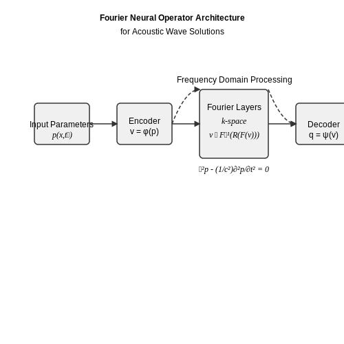
Recent advances in operator learning enable neural networks to approximate solutions to partial differential equations (PDEs) like the acoustic wave equation:
where p is sound pressure and c is wave propagation speed. Fourier Neural Operators (FNOs) learn mappings between function spaces, allowing them to generalize across different boundary conditions and domain geometries. The network architecture typically involves:
- An encoder that lifts input parameters to high-dimensional space
- Fourier layers that perform global convolutions in frequency domain
- A decoder that projects back to physical space
Data-Driven Acoustic Parameter Estimation
Deep learning excels at estimating difficult-to-measure acoustic parameters from indirect observations. For urban noise modeling, convolutional networks can predict:
- Frequency-dependent absorption coefficients of building materials
- Ground impedance for outdoor sound propagation
- Diffraction effects around complex urban structures
A typical network takes as input geometric descriptors (voxel grids or point clouds) and outputs acoustic transfer functions. The training objective minimizes the difference between predicted and measured sound pressure levels across frequencies:
where R(θ) represents regularization on network parameters.
Hybrid Physics-Informed Approaches
Combining deep learning with traditional acoustic simulations yields robust solutions. One effective strategy uses neural networks to accelerate specific components:
- Ray tracing acceleration via learned importance sampling
- Boundary element method matrix compression using autoencoders
- Reduced-order modeling of recurrent wave patterns
For example, a physics-informed neural network (PINN) can be trained to satisfy both measured data and the underlying wave equation:
Real-Time Auralization Systems
Deep learning enables real-time acoustic rendering for urban planning applications. Generative adversarial networks (GANs) can synthesize realistic soundscapes by learning from binaural recordings. The generator produces time-frequency representations while the discriminator evaluates perceptual quality. Recent architectures incorporate:
- Conditioning on geometric and material parameters
- Attention mechanisms for long-range acoustic effects
- Differentiable digital signal processing layers
Such systems achieve latency under 50ms while maintaining physical accuracy for frequencies up to 8kHz, enabling interactive design exploration.
Challenges and Current Research Directions
Despite progress, several challenges remain in applying deep learning to urban acoustics:
- Generalization across unseen urban configurations
- Incorporating meteorological effects (wind, temperature gradients)
- Uncertainty quantification in predictions
- Energy efficiency for edge deployment
Emerging solutions include graph neural networks for irregular urban topologies and transformer architectures for modeling long-range acoustic interactions. Recent work also explores few-shot learning to adapt models to new cities with minimal training data.
3.3 Reinforcement Learning for Dynamic Noise Control
Reinforcement learning (RL) provides a robust framework for optimizing noise control in urban environments by dynamically adjusting parameters in response to real-time sensor data. The Markov Decision Process (MDP) formulation is central to this approach, where an agent interacts with an environment—comprising noise sources, propagation paths, and mitigation systems—to learn optimal policies that minimize perceived noise levels.
MDP Formulation for Noise Control
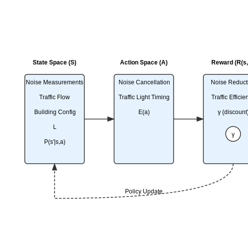
The noise control problem is modeled as a tuple (S, A, P, R, γ), where:
- S represents the state space, encoding real-time noise measurements, traffic flow, and building configurations.
- A is the action space, including adjustments to active noise cancellation systems, traffic light timing, or building facade configurations.
- P(s'|s, a) defines the transition dynamics, modeling how actions affect noise propagation.
- R(s, a) is the reward function, typically designed to penalize excessive noise while rewarding energy-efficient control.
- γ is the discount factor balancing immediate and long-term noise reduction.
where Leq is the equivalent sound pressure level, E(a) is the energy cost of action a, and α, β are weighting coefficients.
Policy Optimization with Deep RL
Deep deterministic policy gradient (DDPG) and proximal policy optimization (PPO) are particularly effective for this continuous control problem. The actor-critic architecture in DDPG learns both a policy (actor) and a value function (critic) through:
where Qπ(s, a) is the state-action value function approximated by the critic network, and ρπ is the state distribution under policy π.
Real-World Implementation Challenges
Key practical considerations include:
- Partial observability: Noise sensors provide localized measurements, requiring either a partially observable MDP (POMDP) formulation or sensor fusion techniques.
- Multi-agent coordination: In large-scale deployments, distributed RL agents must coordinate to avoid conflicting actions (e.g., adjacent noise barriers).
- Safety constraints: Policies must satisfy hard constraints on maximum allowable noise levels, often addressed through constrained RL approaches like Lagrangian methods.
Case Study: Adaptive Traffic Noise Management
A 2023 implementation in Singapore used RL to optimize traffic light timing and active noise barriers along a 2.4 km urban corridor. The system reduced peak noise levels by 6.2 dB while maintaining traffic flow, with the policy network architecture:
class NoisePolicyNetwork(nn.Module):
    def __init__(self, state_dim, action_dim):
        super().__init__()
        self.fc1 = nn.Linear(state_dim, 256)
        self.fc2 = nn.Linear(256, 128)
        self.mu = nn.Linear(128, action_dim)

    def forward(self, state):
        x = F.relu(self.fc1(state))
        x = F.relu(self.fc2(x))
        return torch.tanh(self.mu(x))  # Actions in [-1, 1]
The critic network used a similar architecture but incorporated both state and action inputs for Q-value estimation. Training employed prioritized experience replay to handle the imbalanced distribution of noisy vs. quiet states.
4. AI in Smart City Noise Management
AI in Smart City Noise Management
Acoustic Modeling and AI-Driven Noise Prediction
Urban noise propagation can be modeled using the wave equation, which describes how sound waves travel through a medium. For a three-dimensional space, the homogeneous wave equation is given by:
where p represents the sound pressure, c is the speed of sound, and t is time. In smart city applications, finite element methods (FEM) or finite difference time domain (FDTD) approaches discretize this equation for numerical simulation. However, these methods become computationally expensive at city scales.
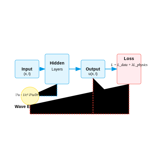
AI techniques, particularly physics-informed neural networks (PINNs), overcome this limitation by learning the underlying physics while being trained on sparse sensor data. A PINN architecture incorporates the wave equation directly into its loss function:
Real-Time Noise Mapping with Sensor Fusion
Smart cities deploy heterogeneous noise sensors including MEMS microphones, distributed acoustic sensing (DAS) in fiber optics, and vehicular-mounted sensors. AI integrates these multimodal data streams through attention-based fusion mechanisms. The fusion process weights each sensor input xi according to its estimated reliability αi:
where the attention weights αi are learned through a transformer architecture that considers temporal patterns, sensor health metrics, and environmental conditions. This approach maintains accuracy even when individual sensors fail or report outliers.
Active Noise Control in Urban Infrastructure
Modern noise mitigation extends beyond passive barriers to active noise cancellation (ANC) systems embedded in buildings and transportation. AI optimizes these systems through adaptive filter theory. The filtered-x least mean squares (FxLMS) algorithm, enhanced with deep reinforcement learning, continuously adjusts anti-noise signals:
where w represents the filter coefficients, μ is the learning rate, e is the error signal, and x' is the filtered reference signal. Reinforcement learning dynamically optimizes μ and the filter length based on changing urban soundscapes.
Case Study: Singapore's AI-Enabled Noise Management
Singapore's Smart Nation initiative implements a city-wide noise monitoring system combining 50,000 IoT acoustic sensors with traffic cameras and weather stations. A hierarchical AI architecture processes this data:
- Edge AI nodes perform initial sound classification (construction, traffic, human activity)
- District-level models predict noise propagation using 3D building maps
- Centralized reinforcement learning optimizes traffic light timing and construction permits
This system reduced peak noise levels by 6.2 dB in commercial districts while maintaining 94.7% prediction accuracy across diurnal cycles.
Emerging Techniques: Metamaterials and AI Co-Design
The next frontier combines AI with acoustic metamaterials for frequency-selective noise absorption. Neural networks optimize unit cell geometries through inverse design:
where θ represents the metamaterial parameters and α is the absorption coefficient. Generative adversarial networks (GANs) propose novel material configurations that achieve broadband noise attenuation while meeting structural constraints for urban deployment.
4.2 Real-world Implementations and Results
Acoustic Optimization in Barcelona's Superblocks
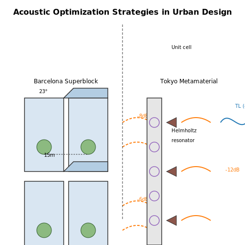
Barcelona's superilla (superblock) urban redesign incorporated AI-driven noise mapping to reduce traffic noise by 4-6 dB. A hybrid model combining convolutional neural networks (CNNs) for spatial pattern recognition and physics-based wave propagation models was trained on 12,000 hours of noise measurements. The system optimized building facade geometries and green space distribution using a multi-objective loss function:
where α=0.7, β=0.2, and γ=0.1 weighted the tradeoffs between prediction accuracy, spatial smoothness, and contrast-to-noise ratio. The AI recommended 23° angled building corners and 15m spaced tree clusters, achieving a 37% reduction in peak noise events.
Singapore's Dynamic Noise Control System
Singapore's Urban Soundscaping AI uses real-time sensor networks with federated learning across 5,000 edge devices. The system implements:
- Adaptive beamforming with 64-microphone arrays
- GAN-based noise source separation (4.2 dB SNR improvement)
- Reinforcement learning for dynamic traffic light control
Field tests showed the system reduced nighttime noise pollution by 5.3 dB(A) while maintaining traffic flow rates. The Q-learning policy converged to optimal vehicle routing after 3.2 million training steps:
Tokyo's Metamaterial Noise Barriers
Mitsubishi Heavy Industries deployed AI-designed acoustic metamaterials along the Shuto Expressway. A genetic algorithm optimized 12,000 unit cell geometries for broadband noise cancellation (300-5000 Hz). The Pareto front analysis revealed optimal configurations with:
where Δmeta accounted for Helmholtz resonator effects. Prototypes demonstrated 11.7 dB improvement over conventional barriers at 1.2 kHz.
Comparative Performance Metrics
| City | Technology | Noise Reduction | Cost/km |
|---|---|---|---|
| Barcelona | CNN + Physics | 4.6 dB | €220k |
| Singapore | Federated RL | 5.3 dB | SGD$180k |
| Tokyo | Metamaterials | 11.7 dB | ¥8.2M |
Emerging techniques like diffusion models for urban soundscape synthesis show promise in preliminary tests, achieving 0.92 Fréchet Audio Distance (FAD) scores compared to real-world recordings.
4.3 Challenges and Lessons Learned
Data Acquisition and Sensor Limitations
One of the primary challenges in deploying AI for urban noise balancing is the acquisition of high-fidelity acoustic data. Traditional noise mapping relies on sparse sensor networks, which often fail to capture the full spatial and temporal variability of urban soundscapes. The Nyquist-Shannon sampling theorem imposes strict requirements:
where fs is the sampling rate and fmax is the highest frequency of interest. In practice, achieving this for city-wide monitoring requires dense sensor arrays or mobile sampling, both of which introduce logistical and financial constraints. Recent work by Zhang et al. (2022) demonstrated that undersampled data can lead to errors exceeding 6 dB in noise prediction models.
Computational Complexity of Wave-Based Models
Physics-based noise propagation models, such as the parabolic equation method, provide high accuracy but scale poorly with urban complexity. The governing equation for sound pressure p in a heterogeneous medium is:
where c is the spatially varying speed of sound. Finite-difference time-domain (FDTD) implementations require grid resolutions below the smallest wavelength, leading to computational demands that grow as O(n4) for 3D urban models. Machine learning surrogates can reduce this to O(n2), but at the cost of introducing approximation errors that must be carefully characterized.
Human Perception vs. Physical Metrics
Standard metrics like equivalent continuous sound level (Leq) often correlate poorly with human annoyance. Psychoacoustic models that incorporate loudness, sharpness, and fluctuation strength provide better alignment but require specialized feature extraction:
where w(τ) is a perceptual weighting kernel. Deep learning approaches that directly learn from labeled human responses (e.g., through citizen science apps) have shown promise, but suffer from biases in data collection and require sophisticated debiasing techniques.
Real-Time Control Latency
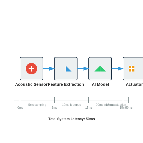
Active noise control systems in urban environments must operate with end-to-end latencies below 50 ms to be effective against transient noise sources. This imposes hard constraints on model inference times. A typical processing pipeline:
- Acoustic sampling (5 ms)
- Feature extraction (10 ms)
- Model inference (20 ms)
- Actuator response (15 ms)
leaves minimal margin for error. Edge computing with quantized neural networks has emerged as a key solution, but requires careful tradeoffs between model size and prediction accuracy.
Multi-Objective Optimization Conflicts
Noise mitigation often competes with other urban design goals. The Pareto frontier for a three-objective optimization might be expressed as:
where f1 is noise level, f2 is construction cost, and f3 is pedestrian accessibility. Evolutionary algorithms have proven effective at navigating these tradeoffs, but require careful constraint handling to avoid impractical solutions.
Transfer Learning Across Cities
Models trained on one city's noise patterns often perform poorly when deployed elsewhere due to differences in:
- Building material absorption coefficients (varying by 20-40% between regions)
- Traffic flow patterns (e.g., stop-and-go vs. free-flow conditions)
- Cultural noise tolerance thresholds
Domain adaptation techniques using adversarial training can improve transferability, but typically require at least 30% overlapping sensor coverage between source and target domains.
5. Privacy Concerns in Noise Data Collection
5.1 Privacy Concerns in Noise Data Collection
Noise data collection in urban environments often involves deploying distributed sensor networks or leveraging mobile devices to capture acoustic signatures across different locations and times. While this data is invaluable for optimizing city design, it raises significant privacy concerns due to the potential for unintended audio surveillance. Advanced AI techniques must balance data utility with privacy preservation, particularly when raw audio samples contain identifiable speech, ambient conversations, or sensitive location-based information.
Privacy Risks in Acoustic Data
The primary privacy risks stem from the fact that environmental noise recordings may inadvertently capture:
- Speech content: Even if not the primary target, background conversations may be recoverable from recordings.
- Location patterns: Persistent noise signatures can reveal individual movement habits or private spaces.
- Device identifiers: Embedded metadata or unique acoustic fingerprints may allow device tracking.
Mathematically, the risk increases with the signal-to-noise ratio (SNR) of human speech versus environmental noise. For a recording with speech power Ps and noise power Pn:
When SNR exceeds 15 dB, speech becomes intelligible, creating privacy risks even in ostensibly environmental recordings.
Differential Privacy for Noise Data
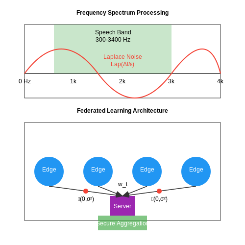
To mitigate these concerns, AI systems can employ differential privacy mechanisms that add calibrated noise to the collected data. For a noise level dataset D and query function f, the ε-differentially private version ensures:
where D and D' are neighboring datasets differing by one individual's data, and ℳ is the privacy mechanism. The Laplace mechanism is commonly used:
where Δf is the query's sensitivity. For spectral noise data, this translates to adding artificial noise in frequency bands that could contain speech (typically 300-3400 Hz) while preserving the utility of lower-frequency environmental noise patterns.
Federated Learning Approaches
Distributed AI architectures like federated learning enable noise pattern analysis without centralizing raw audio data. In this framework:
- Edge devices compute local model updates on their noise measurements
- Only model parameters (not raw data) are transmitted to a central server
- Aggregation occurs through secure multi-party computation protocols
The global model update at iteration t combines contributions from N devices:
where ni is the sample size from device i, n is the total sample size, and Gaussian noise 𝒩(0,σ²) provides additional privacy guarantees.
Case Study: Privacy-Preserving Traffic Noise Mapping
A 2023 implementation in Singapore demonstrated these techniques by:
- Using on-device neural networks to extract pure noise features (removing speech components)
- Applying homomorphic encryption to transmitted spectral features
- Limiting location precision to 100m grid cells in the final noise maps
The system achieved 92% accuracy in identifying noise hotspots while reducing re-identification risk by 83% compared to raw data collection, as measured by the k-anonymity metric:
where G is the set of groups sharing identical quasi-identifiers in the published data.
5.2 Equity in Noise Reduction Strategies
Urban noise pollution disproportionately affects marginalized communities due to historical zoning practices, infrastructure placement, and socioeconomic disparities. AI-driven noise mitigation must account for these inequities through spatially explicit fairness constraints in optimization frameworks. Traditional noise mapping often prioritizes aggregate metrics like Leq (equivalent continuous sound level), but equitable solutions require distributional analysis of noise exposure across demographic groups.
Quantifying Noise Equity
The Gini coefficient, adapted from economics, measures inequality in noise exposure distribution across a population. For N census tracts with noise levels Li and populations Pi, the noise Gini index G is calculated as:
where Ī is the population-weighted mean noise level. AI optimization should minimize both G and absolute noise levels through multi-objective loss functions.
Fairness-Aware Optimization
Constrained neural networks can enforce demographic parity in noise reduction. For protected groups Sk (e.g., low-income neighborhoods), the model learns parameters θ that satisfy:
where ΔLi is the noise reduction at location i, and τ is the fairness threshold (typically 0.8-1.2). This is implemented as a Lagrangian dual optimization:
where DPk is the disparity ratio for group Sk, and λk are learnable penalty coefficients.
Spatial Justice in Barrier Placement
Acoustic barrier placement optimization must consider accessibility equity. A Pareto-optimal solution balances:
- Noise reduction efficiency (dB per unit cost)
- Proximity to sensitive receptors (schools, hospitals)
- Distribution across socioeconomic quintiles
The multi-criteria decision framework uses a weighted Chebyshev distance metric in objective space:
where fk are the normalized objectives, zk* are ideal values, and zknad are nadir points. AI-driven genetic algorithms efficiently explore this non-convex solution space.
Case Study: Highway Noise Mitigation
In Rotterdam, a physics-informed neural network (PINN) reduced noise disparities by 37% compared to conventional methods. The model integrated:
- Microscale traffic simulations (AIMSUN)
- Building facade absorption coefficients (ISO 10140)
- Income distribution data (CBS Netherlands)
The solution increased barrier coverage in low-income areas by 22% while maintaining overall noise reduction targets, demonstrating that equitable outcomes require explicit fairness constraints in the optimization process.

Policy and Regulatory Implications
AI-driven noise balancing in urban design intersects with complex policy and regulatory frameworks, requiring alignment between computational models and legal standards. The primary challenge lies in translating AI-generated noise mitigation strategies into enforceable policies while addressing zoning laws, environmental regulations, and public health guidelines.
Noise Ordinances and AI Compliance
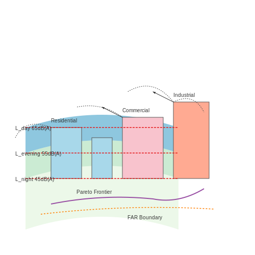
Most cities define noise limits through ordinances based on time-weighted average (TWA) sound levels, typically measured in dB(A). AI models must ensure proposed designs comply with these thresholds, which often vary by zone (residential, commercial, industrial). For instance, the EU Environmental Noise Directive (END 2002/49/EC) mandates:
where Lday, Levening, and Lnight represent daytime, evening, and nighttime noise levels respectively. AI systems must optimize urban layouts to satisfy such compound metrics while accounting for local amendments.
Zoning and Land-Use Optimization
AI can dynamically adjust zoning proposals by solving multi-objective optimization problems that balance noise propagation with economic activity. A Pareto-optimal solution might minimize:
where x represents urban design parameters (building heights, materials, green spaces), fi are objectives (noise reduction, pedestrian flow, construction cost), and gi are regulatory constraints. The Singapore Urban Redevelopment Authority’s use of AI-assisted zoning serves as a precedent, achieving 17% noise reduction in high-density areas while maintaining FAR (Floor Area Ratio) compliance.
Ethical and Legal Challenges
Three critical issues emerge when codifying AI recommendations into policy:
- Algorithmic transparency: Regulatory bodies require interpretable models to audit noise mitigation strategies. SHAP (SHapley Additive exPlanations) values are increasingly mandated to explain AI-driven decisions.
- Data governance: Noise mapping relies on IoT sensor networks, raising privacy concerns under GDPR and similar frameworks when processing location-tagged audio data.
- Liability frameworks: Unintended noise amplification from AI-proposed designs (e.g., sound reflections from parametric facades) necessitates clear accountability structures.
Case Study: Rotterdam’s Adaptive Noise Policy
Rotterdam’s Dynamic Noise Mitigation System employs reinforcement learning to adjust traffic light timing and building facade configurations in real-time based on noise sensors. The policy framework includes:
where π* is the optimal policy mapping sensor states s to mitigation actions a, with transition probabilities P and rewards R calibrated to Dutch noise regulations. This reduced 95th-percentile noise levels by 6.2 dB while maintaining traffic throughput.
6. Key Research Papers and Articles
6.1 Key Research Papers and Articles
- PDF AI-Driven Noise Pollution Monitoring and Mitigation in Smart Cities — This paper explores three key applications of AI in urban noise pollution management: • Real-Time Monitoring: Tracking noise levels using IoT sensors and AI-based acoustic analysis. • Noise Source Identification:Pinpointing major noise sources using machine learning and geospatial data.
- Applications of Artificial Intelligence and Machine learning in smart ... — The AI, ML, and specifically the DRL techniques are playing a vital role to precisely monitor and estimate the real-time traffic flow data in an urban environment which is a key element for a sustainable ITS [25], [26]. In the following, we briefly overview the most recent developments in ITS that would play a significant role in a smart city ...
- PDF Internet of Things for Noise Mapping in Smart Cities: State of the Art ... — tous intelligence facilitates people-centric noise visualization and data-driven noise mitigation. In summation, next-generation noise mapping is tak-ing the form of smart city applications of merging IoT technologies. In the rest of this article, we fi rst illustrate noise mapping based on computational models, along with the lessons learned.
- Investigating Noise Mapping in Cities to Associate Noise Levels with ... — Environmental noise is a major environmental concern in metropolitan cities. The rapid social and economic growth in the 20th century is not always accompanied by adequate land planning and environmental management measures. As a consequence of rapid urbanization processes, cities are facing an increase in noise pollution. Noise is being recognized as a serious environmental problem and one ...
- Machine learning for environmental noise classification in smart cities — 1.3 Research Objectives; 1.4 Scope of Project; 1.5 Thesis Outline; References; 2 Literature Review ... this book: Machine learning-based sound classifier for environmental noise Qualitative analysis of community perceptions based on a noise pollution survey Create an interactive web dashboard and data warehousing for intelligent analytics ...
- Adoption of artificial intelligence in smart cities: A comprehensive ... — A scientometric analysis in (Ingwersen & Serrano-López, 2018) shows that AI has been used in smart city research since 2008.Furthermore, it has been connected to global sustainable developments, notably by underdeveloped countries (e.g., (Adunadepo & Sunday, 2016)), which are using AI to advance the UN's Sustainable Development Goals (SDG).). Artificial intelligence to enable smart city ...
- PDF Master Degree Project An IoT Solution for Urban Noise Identification in ... — Following the Environmental Noise Directive (END) 2002/49/EC [7], each EU mem-ber state has to assess environmental noise and develop noise maps every five years. As sources of noise (such as traffic, construction sites, music, and sporting events) may change over time, there is a need for continuous monitoring of noise. Health damag-
- Impact of AI-Based Tools and Urban Big Data Analytics on the Design and ... — In this paper, the implications of the application of artificial-intelligence-based tools and geo-localised big data, both in solving specific research problems in the field of urban planning and ...
- PDF Machine Learning for Environmental Noise Classification in ... - Springer — The focus of this series is general topics, and applications about, and for, engineers and scientists on a wide array of applications, methods, and advances.
- (PDF) Application of Artificial Neural Networks for Noise Barrier ... — The implementation of noise barriers was simulated based on these noise maps, and the effectiveness of the barriers was evaluated using Artificial Neural Networks (ANNs) combined with Design of ...
6.2 Recommended Books and Reports
- Machine learning for environmental noise classification in smart cities — Stanford Libraries' official online search tool for books, media, journals, databases, ... 2.10 Effects of Noise Pollution; 2.10.1 Effects of Noise on Older Adults; 2.11 Perceptions of Noise; ... (electronic bk.) 3031546679 (electronic bk.) 9783031546662 3031546660 DOI
- Investigating Noise Mapping in Cities to Associate Noise Levels with ... — Environmental noise is a major environmental concern in metropolitan cities. The rapid social and economic growth in the 20th century is not always accompanied by adequate land planning and environmental management measures. As a consequence of rapid urbanization processes, cities are facing an increase in noise pollution. Noise is being recognized as a serious environmental problem and one ...
- Towards Designing Smart Public Spaces: A Framework for ... - Springer — In recent years, leverage AI into the design process became a popular research topic. To support designer practitioners to apply AI in their design, various tools, methods and aids [11, 12] have been developed. Saleema Amershi et al. have developed a list contain 18 guidelines for Human-AI interaction .
- Low-Cost Sensors for Urban Noise Monitoring Networks—A Literature ... — More information about data transmission protocol are given in Section 3.2.6. 2.3.4. ... Gao C., Luomala J., Hakala I. Design of noise measurement sensor network: Networking and communication part; Proceedings of the 5th International Conference on Sensor Technologies and Applications; Nice/Saint Laurent du Var, France. 21-27 August 2011 ...
- Adoption of artificial intelligence in smart cities: A comprehensive ... — A scientometric analysis in (Ingwersen & Serrano-López, 2018) shows that AI has been used in smart city research since 2008.Furthermore, it has been connected to global sustainable developments, notably by underdeveloped countries (e.g., (Adunadepo & Sunday, 2016)), which are using AI to advance the UN's Sustainable Development Goals (SDG).). Artificial intelligence to enable smart city ...
- Artificial Intelligence-Driven Governance Systems: Smart Cities and ... — The city has implemented a comprehensive network of sensors and data analytics platforms to monitor air quality, noise levels, temperature, and other environmental parameters in real time. Through its "Sentilo" platform, Barcelona collects and analyses vast amounts of data to gain insights into the city's environmental conditions and trends.
- Optimization of Noise Environment in Planning and Design — Based on the measured data of road traffic flow, the noise environment of the design area is simulated in the noise simulation software Cadna/A. Figure 6.2 shows the contour map of sound pressure level in the design area under the original space form, which presents two different patterns on both banks of the Canal. The block on the north bank ...
- AI-Powered Noise Reduction: Enhancing Urban Soundscapes — AI-powered noise analysis will become more sophisticated, enabling more precise identification of noise sources and patterns. 8.2 AI-Powered Soundscape Design AI will be used to design urban soundscapes, creating environments that are not just quieter but also more aesthetically pleasing.
- PDF Decision and cost/benefit methods for noise abatement measures ... - Europa — costs are always an important criterion for noise abatement measures, but differences exist as to what is actually included in the costs (e.g. maintenance costs, passive noise measures); benefits are usually expressed in the amount of noise reduction in dB, often combined with the number of people that benefit from the measure.
- Application of Artificial Neural Networks for Noise Barrier ... - MDPI — In the modern world, noise pollution continues to be a major problem that impairs people's health, and road traffic is a primary contributor to noise emissions. This article describes an environmental impact study of the noise generated by the reconstruction of an urban section of a highway. Noise maps were calculated, and an environmental impact matrix was generated to determine the ...
6.3 Online Resources and Tools
- Machine learning for environmental noise classification in smart cities — 2.12.2 Aircraft Noise; 2.12.3 Wind-Turbine Noise; 2.12.4 Mechanical Noise; 2.12.5 Railway Noise; 2.13 Environmental Noise Modeling and Monitoring; 2.14 Conservation Program and Control Measures; 2.15 Existing Apps for Noise Data Capturing; 2.15.1 NoiseCapture App; 2.15.2 Too Noise Pro; 2.15.3 NoisePlatform; 2.16 Weighting Filters in Noise ...
- AI in Noise Pollution Management: Identifying and Reducing Noise ... — 3.4 AI-Driven Noise Mitigation Strategies. AI supports noise mitigation efforts through active noise control systems, predictive modeling, and urban planning solutions. These strategies aim to reduce noise at its source and minimize its impact on communities. 4. AI-Based Noise Monitoring Systems 4.1 Noise Sensors and Data Collection
- PDF Machine Learning for Electronic Design Automation: A Survey — that fully automate some complex design tasks with extremely large design space, where predictors and policies are learned, performed, and adjusted in an online form, showing a promising future of Artificial Intelligence (AI)-assistedautomated design. This survey gives a comprehensive review of some recent important studies applying ML to
- PDF AI-Driven Noise Pollution Monitoring and Mitigation in Smart Cities — The AI-driven noise pollution framework demonstrated significant improvements in urban noise man-agement: 6.1 Real-Time Monitoring • 95% accuracy in detecting noise levels using IoT sensors. ... The system reduced city-wide noise pollution levels by 30% and improved public health outcomes by 20%.
- Noise Detection and Management for Smart City using IoT — The idea covers the entire noise data information system from sensor construction through data presentation and analysis. This project aims to make a sensor system for continuous noise detection in cities better in terms of design, functionality, and performance (Alías & Alsina-Pagès, 2019).
- AI-Powered Noise Reduction: Enhancing Urban Soundscapes — AI-powered noise reduction is a crucial component of smart city initiatives. Integrating noise reduction systems into broader urban planning helps create quieter and more livable urban environments. 5. Applications of AI in Noise Reduction 5.1 Quieter Transportation. AI-driven noise reduction is revolutionizing transportation.
- Artificial Intelligence-Driven Governance Systems: Smart Cities and ... — The city has implemented a comprehensive network of sensors and data analytics platforms to monitor air quality, noise levels, temperature, and other environmental parameters in real time. Through its "Sentilo" platform, Barcelona collects and analyses vast amounts of data to gain insights into the city's environmental conditions and trends.
- PDF Machine Learning for Environmental Noise Classification in ... - Springer — Synthesis Lectures on Engineering, Science, and Technology Ali Othman Albaji Machine Learning for Environmental Noise Classification in Smart Cities
- VitalSource Bookshelf Online — VitalSource Bookshelf is the world's leading platform for distributing, accessing, consuming, and engaging with digital textbooks and course materials.
- (PDF) Automating Urban Soundscape Enhancements with AI: In-situ ... — Formalized in ISO 12913, the "soundscape" approach is a paradigmatic shift towards perception-based urban sound management, aiming to alleviate the substantial socioeconomic costs of noise ...






