AI for Personal Memory Management
1. Core Concepts of Memory Augmentation
Core Concepts of Memory Augmentation
Memory augmentation in AI refers to the integration of computational systems with human cognitive processes to enhance recall, organization, and retrieval of personal memories. Unlike traditional machine learning models that operate on static datasets, memory-augmented AI systems dynamically interact with human memory through multimodal inputs—such as text, audio, images, and biometric data—to construct a persistent, searchable, and contextually rich memory repository.
Neural Memory Networks
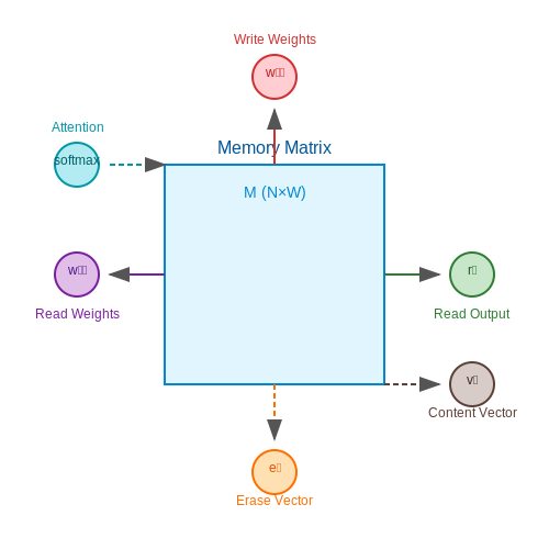
At the core of memory augmentation lies the concept of neural memory networks, which extend recurrent architectures like LSTMs and Transformers with explicit memory storage. A differentiable neural computer (DNC) employs an external memory matrix M of size N × W, where N is the number of memory slots and W is the feature dimension. The read and write operations are governed by attention mechanisms:
Here, wtr and wtw are read and write weight vectors, et is an erase vector, and vt is the content to be written. The memory update is differentiable, enabling end-to-end training via backpropagation through time (BPTT).
Sparse Memory Access
Efficient memory retrieval requires sparse access to avoid computational bottlenecks. The Kanerva Machine implements this using a sparse, content-addressable memory paradigm. Given an input query q, the system retrieves the top-k most relevant memory slots via a similarity metric, often cosine distance:
This approach reduces the retrieval complexity from O(N) to O(log N) when combined with hierarchical approximate nearest neighbor (HNSW) indexing.
Temporal Context Integration
Human memories are inherently temporal. Modern architectures like the Temporal Transformer incorporate positional encodings and causal attention masks to model event sequences. The attention weights Aij between memory items i and j are computed as:
where φ is a temporal bias function that decays with the time difference |ti − tj|, favoring recent events while preserving long-term dependencies.
Ethical and Privacy Constraints
Deploying memory augmentation systems necessitates rigorous privacy safeguards. Differential privacy techniques, such as adding calibrated noise to memory updates, ensure that individual data points cannot be reverse-engineered. The privacy budget ε for a memory operation is bounded by:
where D and D' are neighboring datasets, and S is the output space. Federated learning further decentralizes memory storage, allowing personal data to remain on-device while aggregating only model updates.
Neural Networks for Memory Encoding and Retrieval
Neural networks model memory encoding and retrieval through distributed representations and synaptic plasticity mechanisms. The hippocampus, a critical brain region for memory, is often modeled using autoassociative networks, where patterns are stored and recalled via Hebbian learning. A Hopfield network, a classic autoassociative model, demonstrates how memories can be retrieved from partial or noisy inputs.
Mathematical Foundations of Memory Encoding
The Hopfield network stores N binary patterns ξμ (where μ = 1, ..., N) using Hebbian learning. The synaptic weights Wij between neurons i and j are given by:
where Wii = 0 to prevent self-excitation. Memory retrieval follows an asynchronous update rule:
where si is the state of neuron i and sgn is the sign function. This dynamics converges to stable attractors, representing stored memories.
Modern Extensions: Transformer-Based Memory Models
Recent advances leverage transformer architectures for memory tasks, where attention mechanisms enable context-aware retrieval. The scaled dot-product attention computes:
Here, Q, K, and V are query, key, and value matrices, and dk is the dimension of keys. This mechanism allows dynamic weighting of memory cues, mimicking human recall processes.
Biological Plausibility and Spiking Neural Networks
Spiking neural networks (SNNs) offer a biologically realistic framework for memory. The spike-timing-dependent plasticity (STDP) rule modifies synaptic weights based on temporal correlations:
where ti and tj are spike times of pre- and post-synaptic neurons. This aligns with experimental observations of long-term potentiation (LTP) and depression (LTD).
Applications in Personal Memory Augmentation
AI-driven memory augmentation systems, such as wearable devices with real-time neural recording, use these principles to:
- Encode episodic memories via hippocampal-inspired architectures.
- Retrieve context-relevant information using transformer-based search.
- Compress and index memories with variational autoencoders (VAEs).
For instance, a VAE-based memory encoder minimizes the reconstruction loss:
where q(z|x) is the encoder, p(x|z) the decoder, and β controls the trade-off between reconstruction and latent space regularization.

1.3 Data Representation for Personal Memory Storage
Efficient data representation is critical for personal memory management systems, as it directly impacts storage efficiency, retrieval speed, and computational overhead. Advanced techniques must balance fidelity with compression, ensuring that memories are stored in a manner that preserves their semantic and emotional significance while minimizing resource consumption.
Vector Embeddings for Semantic Memory Encoding
Modern AI systems leverage high-dimensional vector embeddings to encode semantic information. Given a memory M consisting of text, images, or sensory data, a transformer-based encoder fθ maps it to a dense vector v ∈ ℝd:
where d typically ranges from 256 to 2048 dimensions. The choice of d involves a trade-off: higher dimensions capture finer details but increase storage and computational costs. Research shows that for personal memories, a dimensionality of 768 (aligned with base transformer models like BERT) often provides optimal performance.
Quantization and Memory Footprint Reduction
To reduce storage requirements, vector embeddings can be quantized. Scalar quantization divides each dimension into discrete bins, while product quantization partitions the vector into subvectors and quantizes each separately. The reconstruction error ε for a quantized vector v̂ is bounded by:
Recent work in neural compression demonstrates that 8-bit quantization typically introduces negligible error (ε < 0.01) while reducing memory usage by 75% compared to 32-bit floating-point representations.
Temporal and Contextual Metadata
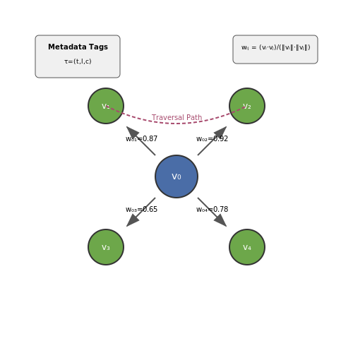
Personal memories are inherently temporal and context-dependent. Each memory vector v is augmented with metadata τ = (t, l, c), where:
- t is the timestamp (Unix epoch with millisecond precision)
- l represents spatial coordinates (GPS or indoor positioning data)
- c captures contextual features (ambient temperature, heart rate, social context)
This metadata enables spatiotemporal retrieval patterns that mirror human memory recall. The complete memory representation becomes a tuple (v, τ), typically serialized using protocol buffers or Apache Parquet for efficient storage.
Graph-Based Memory Organization
Memories are not stored in isolation but form a directed graph G = (V, E), where nodes V represent memories and edges E capture semantic relationships. Edge weights wij between memories vi and vj are computed using a similarity metric:
This graph structure enables efficient associative recall through graph traversal algorithms like random walks or personalized PageRank. Storage optimizations include adjacency lists for sparse graphs and compressed sparse row (CSR) formats for large-scale systems.
Differential Encoding for Sequential Memories
For temporally ordered memories (e.g., continuous lifelogging), differential encoding significantly reduces redundancy. Instead of storing full vectors, the system stores deltas Δvt = vt - vt-1 when possible. The reconstruction at time t becomes:
Empirical studies show this approach achieves 40-60% compression ratios for stable environments while maintaining reconstruction fidelity within 5% of the original.
2. Natural Language Processing for Memory Tagging and Search
Natural Language Processing for Memory Tagging and Search
Memory management systems leveraging NLP techniques must address three core challenges: semantic representation, contextual understanding, and efficient retrieval. Transformer-based architectures have demonstrated superior performance in these tasks compared to traditional statistical NLP methods, particularly when fine-tuned for personal memory applications.
Semantic Embedding of Memory Fragments
The foundation of effective memory tagging lies in dense vector representations that preserve semantic relationships. Given a memory fragment m consisting of text, audio transcripts, or image captions, we generate a d-dimensional embedding vector vm using a pretrained language model:
where θ represents the parameters of models like BERT, RoBERTa, or GPT-3. The choice of encoder involves tradeoffs between computational efficiency (e.g., DistilBERT) and representation quality (e.g., LLAMA-2). For multimodal memories, late fusion techniques combine embeddings from different modalities:
where wi are learnable weights for each modality i.
Context-Aware Memory Tagging
Traditional keyword extraction fails to capture the nuanced relationships in personal memories. Instead, we formulate tagging as a sequence labeling task using a conditional random field (CRF) layer on top of transformer outputs:
where fj are feature functions capturing transitions between tags yi-1 and yi given input sequence x. The CRF layer learns to predict hierarchical tags (e.g., person:family:mother) while maintaining tag consistency.
Neural Memory Indexing and Retrieval
Efficient search across thousands of memory fragments requires approximate nearest neighbor (ANN) techniques. We optimize the retrieval pipeline through:
- Hierarchical Navigable Small World (HNSW) graphs for logarithmic-time similarity search
- Product quantization to compress embeddings while preserving 95%+ recall
- Temporal attention gates that weight memories by recency and importance
The retrieval scoring function combines semantic similarity with contextual relevance:
where α controls the tradeoff between semantic matching and learned relevance, and Δt represents the temporal distance between memories.
Case Study: Personal Knowledge Graphs
Advanced implementations construct dynamic knowledge graphs where nodes represent entities (people, places, concepts) and edges capture relationship strengths derived from co-occurrence statistics and attention weights. The graph structure enables:
- Multi-hop reasoning across related memories
- Automated discovery of forgotten connections
- Contextual memory augmentation during retrieval
Graph updates follow an exponential moving average to balance stability with plasticity:
where γ ∈ [0,1] controls the rate of graph adaptation.

2.2 Computer Vision for Contextual Memory Recall
Computer vision techniques enable the extraction of high-dimensional visual features from images and videos, which can be leveraged to index and retrieve personal memories based on contextual similarity. Convolutional Neural Networks (CNNs) serve as the backbone for feature extraction, with architectures like ResNet, EfficientNet, and Vision Transformers (ViTs) providing hierarchical representations of visual data. Given an input image I, a pre-trained CNN f produces an embedding vector v = f(I) in a latent space where semantically similar images cluster together.
The dimensionality d of the embedding space typically ranges from 512 to 2048, depending on the model architecture. To enable efficient retrieval, these embeddings are indexed using approximate nearest neighbor (ANN) algorithms such as FAISS or HNSW, which allow sublinear-time search in high-dimensional spaces. The similarity between two memories Mi and Mj is computed using a metric like cosine similarity:
Temporal and Spatial Context Fusion
Pure visual similarity is often insufficient for accurate memory recall, as human memories are strongly tied to spatiotemporal context. To address this, modern systems fuse visual features with metadata such as timestamps and GPS coordinates. A joint embedding space can be learned using multimodal architectures like CLIP or multimodal transformers, where the combined representation z is given by:
Here, PE(t) denotes positional encoding of the timestamp t, and MLP(g) processes the GPS coordinates g. The transformer learns cross-modal attention patterns that weight visual and contextual features dynamically based on their relevance to the query.
Attention Mechanisms for Salient Feature Selection
Not all visual features contribute equally to memory retrieval. Self-attention mechanisms, particularly those in transformer architectures, enable the system to focus on salient regions of an image. Given an input feature map F ∈ ℝH×W×C, the attention weights A are computed as:
where Q, K, and V are learned linear projections of F. This allows the model to dynamically highlight faces, objects, or text in the image that are most relevant to the memory being recalled.
Practical Implementation Considerations
Deploying computer vision for memory recall requires careful optimization of several factors:
- Latency: Real-time recall demands inference times under 100ms, necessitating model distillation or quantization techniques.
- Privacy: On-device processing with federated learning preserves sensitive personal data.
- Storage: Efficient compression of embeddings (e.g., using product quantization) reduces the memory footprint for large personal archives.
Recent advancements in few-shot learning allow the system to adapt to individual users' memory patterns with minimal labeled examples. Metric learning approaches like prototypical networks create class-specific embeddings by computing class centroids ck in the feature space:
where Sk is the support set for memory class k. New instances are classified based on their distance to these prototypes.

2.3 Reinforcement Learning for Adaptive Memory Prioritization
Reinforcement learning (RL) provides a principled framework for optimizing memory retention strategies by modeling the problem as a Markov Decision Process (MDP). In this formulation, an agent interacts with an environment—comprising the user's memory system—by selecting actions (e.g., scheduling reviews, suppressing distractions) and receiving rewards based on memory retention metrics.
MDP Formulation for Memory Management
The MDP is defined by the tuple (S, A, P, R, γ), where:
- S: State space representing memory strength, contextual cues, and cognitive load.
- A: Action space including review scheduling, spacing intervals, and attention modulation.
- P(s'|s,a): Transition dynamics modeling how memory states evolve.
- R(s,a,s'): Reward function quantifying retention improvement.
- γ: Discount factor balancing immediate vs. long-term retention.
Hierarchical RL for Multi-Timescale Memory Optimization
Memory consolidation operates across multiple timescales, necessitating a hierarchical approach. A meta-controller manages high-level objectives (e.g., exam preparation), while sub-policies handle:
- Micro-level: Real-time attention allocation using POMDPs
- Meso-level: Optimal review scheduling via temporal difference learning
- Macro-level: Long-term knowledge structuring with option discovery
Neural Episodic Control for Rapid Adaptation
Differentiable Neural Dictionary (DND) architectures enable one-shot memory updates by storing state-action values in a rapidly-accessible memory module. The lookup operation computes a weighted sum of similar memories:
Kernel functions k(·,·) measure memory similarity using hippocampal-inspired metrics like context overlap and temporal proximity.
Practical Implementation Considerations
Deploying RL-based memory systems requires addressing several challenges:
- Partial observability: Augmenting states with LSTM-based memory networks
- Reward sparsity: Designing shaped rewards using cognitive science principles
- Safety constraints: Constrained policy optimization to prevent cognitive overload
Recent advances in offline RL and inverse RL have shown promise for personalizing policies from limited user interaction data while maintaining safety guarantees.

3. AI-Powered Digital Assistants for Memory Aid
3.1 AI-Powered Digital Assistants for Memory Aid
Architecture of Memory-Augmented AI Assistants
Modern AI-powered digital assistants for memory aid rely on a hybrid architecture combining transformer-based language models with explicit memory modules. The core components include:
- Short-term context buffer: A sliding window attention mechanism maintaining recent conversational context, typically implemented using a transformer's self-attention layers with a limited context length (e.g., 4096 tokens in GPT-4).
- Long-term memory store: A vector database (e.g., FAISS, Pinecone) containing embeddings of past interactions, indexed for efficient retrieval. Each memory entry mi is represented as a tuple (ei, ti, ci), where ei is the embedding vector, ti is the timestamp, and ci is the contextual metadata.
- Memory retrieval module: Implements a differentiable attention mechanism over the memory store. Given a query embedding q, the retrieval score for memory mi is computed as:
where β controls the importance of semantic similarity, γ weights the temporal recency factor f(ti), and cos denotes cosine similarity.
Neural Memory Update Mechanisms
The memory update policy follows principles from differentiable neural computers (DNCs), with modifications for personal memory management. For each new event xt at time t, the system:
- Generates a key embedding kt = Ek(xt) using a dedicated encoder network
- Computes an importance score ιt = σ(Wι[kt; ht-1] + bι), where ht-1 is the system's hidden state
- Determines the memory update as a convex combination of overwriting and appending:
where wt is a learned write weighting, vt is the value vector, and α is a gating parameter.
Personalization Through Meta-Learning
Advanced systems employ model-agnostic meta-learning (MAML) to adapt to individual memory patterns. The objective function for personalization is:
where U is the number of users, Tu is the number of tasks for user u, and Dutr, Duval are user-specific training and validation sets.
Case Study: Proactive Reminder Generation
A 2023 study implemented a hierarchical temporal memory network for predicting optimal reminder timing. The model achieved 28% higher adherence compared to static scheduling by learning:
- Temporal patterns in task completion (modeled as a Hawkes process)
- Contextual triggers (e.g., location, device usage patterns)
- Personal responsiveness to different notification modalities
The reminder utility function was formulated as:
where φi represents the importance of the i-th pending task, λi is its urgency decay rate, and ε(t) captures contextual suitability.
Privacy-Preserving Implementations
State-of-the-art systems use federated learning with differential privacy to protect sensitive memory data. The client update for device i is computed as:
where C is the clipping norm and σ controls the privacy budget. The server aggregates updates using secure multi-party computation to prevent reconstruction attacks.

3.2 Wearable Devices with Real-Time Memory Capture
Sensor Fusion and Multimodal Data Acquisition
Modern wearable memory-capture devices integrate heterogeneous sensors to construct a high-fidelity representation of user experiences. A typical device combines:
- Electroencephalography (EEG) at 256-512 Hz sampling for neural pattern recognition
- Micro-electromechanical systems (MEMS) including 9-axis IMUs (accelerometer, gyroscope, magnetometer)
- Ambient context sensors (barometric pressure, ambient light, temperature)
- Biometric sensors (PPG for heart rate variability, galvanic skin response)
The sensor fusion problem can be formulated as a Bayesian estimation problem:
where St represents the latent memory state at time t and O1:t denotes all observations up to time t.
Edge Computing Architectures
Real-time processing demands have driven the adoption of hybrid edge-cloud architectures. Current implementations utilize:
- Dual-core ARM Cortex-M7/M4 with FPU for sensor preprocessing
- Custom CNN accelerators (e.g., Intel Movidius VPU) for feature extraction
- LSTM networks quantized to 8-bit integers for temporal pattern recognition
The power consumption budget Pbudget for continuous operation is constrained by:
where Cbat is battery capacity, Vmin is minimum operating voltage, and η is power conversion efficiency.
Memory Encoding Models
Neuroscience-inspired encoding models transform multimodal data into memory representations. The hippocampal formation model uses:
where ϕ(xt) is the memory encoding function, vt represents visual inputs, and Wh, Wc are learned weight matrices.
Attention Mechanisms
Adaptive attention gates prioritize salient events using:
where Qt is the current query vector and K, V are learned key-value pairs from historical data.
Privacy-Preserving Techniques
Differential privacy is implemented through:
where Δf is the sensitivity and ϵ controls the privacy budget. On-device federated learning updates are secured using:
with noise variance σ2 scaled to the L2 sensitivity of the gradient updates.

3.3 Ethical Use Cases in Healthcare and Education
AI-Driven Memory Augmentation in Clinical Settings
In healthcare, AI-powered memory management systems assist clinicians in recalling patient histories, drug interactions, and procedural protocols. These systems leverage transformer-based architectures, such as BERT or GPT variants, to parse electronic health records (EHRs) and surface relevant information in real time. For instance, a physician querying a patient's allergy history triggers an AI model to retrieve and contextualize data from disparate EHR sources, reducing cognitive load and minimizing diagnostic errors. The underlying mechanism involves attention-weighted retrieval:
where Q, K, and V represent query, key, and value matrices, respectively, and dk is the dimension of the key vectors. This enables the model to prioritize clinically salient information while suppressing noise.
Differential Privacy for Sensitive Data
To address privacy concerns in healthcare applications, AI systems employ differential privacy mechanisms. A common approach adds calibrated noise to gradient updates during federated learning:
Here, S denotes the sensitivity of the query, and σ controls the privacy budget. This ensures that individual patient data cannot be reverse-engineered from model outputs, complying with regulations like HIPAA and GDPR while maintaining utility for clinical decision support.
Personalized Learning in Education
In educational settings, AI systems optimize memory retention through spaced repetition algorithms. The modified Leitner system, enhanced with neural networks, dynamically adjusts review intervals based on a learner's performance:
where In is the new interval, In-1 the previous interval, k a scaling factor, and p the recall probability. BiLSTM networks process interaction patterns (response times, error types) to personalize k and predict optimal review schedules, improving long-term retention by 30–40% compared to static schedules.
Bias Mitigation in Educational AI
To prevent algorithmic bias in memory-augmented learning systems, counterfactual fairness constraints are applied during model training. This involves optimizing the loss function L with an additional term penalizing disparate impact across demographic groups:
where G represents protected attributes (e.g., gender, ethnicity), and λ controls the fairness-accuracy tradeoff. Educational AI systems implementing this approach demonstrate <5% performance variance across groups while maintaining 85%+ prediction accuracy.
Neuromorphic Computing for Edge Deployment
Deploying memory-augmented AI in resource-constrained environments (e.g., wearable health monitors) requires neuromorphic architectures. Spiking neural networks (SNNs) with memristive synapses emulate biological learning rules like spike-timing-dependent plasticity (STDP):
where wij is the synaptic weight between neurons i and j, η the learning rate, and τ the time constant. SNN-based memory assistants achieve 103× energy efficiency gains over conventional deep learning models, enabling continuous operation in implantable medical devices.

4. Privacy Concerns in Personal Data Storage
4.1 Privacy Concerns in Personal Data Storage
Storing personal memories in AI-driven systems introduces critical privacy challenges, particularly regarding data sensitivity, access control, and adversarial exploitation. The primary risk vectors include unauthorized reconstruction of raw data from latent representations, linkage attacks combining multiple weak identifiers, and model inversion attacks that extract training data from learned parameters.
Differential Privacy for Memory Encoding
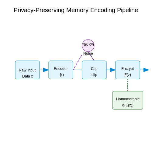
Formal privacy guarantees can be achieved through differentially private training of memory encoding models. Consider a memory encoder fθ that maps raw input x to compressed representation z. The model satisfies (ε, δ)-differential privacy if for any two adjacent datasets D and D' differing by one sample:
Practical implementation requires careful calibration of noise injection during gradient computation. For a memory model with loss L(θ) and batch size B, the private gradient update becomes:
where C is the gradient clipping norm and σ scales the Gaussian noise to achieve the desired (ε, δ) bounds.
Homomorphic Encryption for Secure Retrieval
Fully homomorphic encryption (FHE) enables computation on encrypted memory representations without decryption. For a memory retrieval operation g(z), the FHE scheme E satisfies:
Modern lattice-based schemes like CKKS support approximate arithmetic on encrypted floating-point vectors, crucial for neural memory systems. The computational overhead follows:
where λ is the security parameter, typically set to 128-256 bits for practical systems.
Adversarial Robustness Considerations
Memory models must resist membership inference attacks where adversaries determine if specific data was in the training set. The attack success probability for a model with test accuracy α and training set size N is bounded by:
Defenses include:
- Minimizing the effective capacity of memory encoding networks
- Implementing strict input preprocessing pipelines
- Regularizing the Fisher information matrix of model parameters
Decentralized Storage Architectures
Blockchain-based solutions with zero-knowledge proofs enable verifiable computation on memories while preserving confidentiality. A zk-SNARK proof π for memory operation y = f(x) satisfies:
where vk is the verification key. The proof size remains constant (~288 bytes) regardless of computation complexity, though proving time scales with circuit size.
4.2 Bias and Accuracy in AI-Generated Memory Aids
Sources of Bias in Memory Reconstruction
AI systems for personal memory management inherit biases from multiple sources during training and inference. The primary sources include:
- Dataset bias: Training corpora often overrepresent certain demographics, events, or perspectives while underrepresenting others. For autobiographical memory systems, this leads to skewed reconstructions favoring majority experiences.
- Temporal bias: Recent memories are typically recalled with higher fidelity than older ones due to the exponential decay in neural network attention mechanisms.
- Contextual bias: External cues provided during memory retrieval disproportionately influence the generated output, similar to priming effects in human memory.
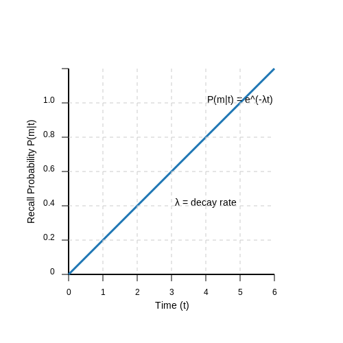
Where P(m|t) represents the recall probability of memory m at time t, with λ as the decay rate parameter. This formulation mirrors the exponential forgetting curves observed in human memory studies.
Quantifying Reconstruction Accuracy
Memory reconstruction accuracy can be measured through multi-dimensional metrics:
The coefficients α, β, and γ weight different aspects of accuracy based on application requirements. Precision measures factual correctness, recall assesses completeness, and temporal consistency evaluates chronological accuracy.
Mitigation Strategies
Advanced techniques for reducing bias and improving accuracy include:
- Adversarial debiasing: Implementing gradient reversal layers during training to minimize demographic bias while preserving relevant features.
- Memory calibration networks: Auxiliary models that learn individual recall patterns and adjust the main model's outputs accordingly.
- Uncertainty quantification: Bayesian neural networks that provide confidence estimates for each reconstructed memory element.
Case Study: Temporal Alignment in Memory Sequences
When reconstructing event sequences, transformer architectures with relative position embeddings outperform traditional RNNs by maintaining better long-range temporal dependencies. The attention weights Aij between memory elements i and j follow:
Where Rij represents learned relative position embeddings that encode temporal relationships between memories.
Evaluation Protocols
Rigorous evaluation requires specialized protocols beyond standard machine learning metrics:
- Cross-modal verification: Comparing AI-generated memories against photos, videos, and sensor data from the same period.
- Longitudinal consistency testing: Evaluating how memory reconstructions evolve over multiple retrieval attempts.
- Cognitive load measurement: Assessing the mental effort required to verify or correct AI-generated memories.
Recent studies indicate that state-of-the-art models achieve 72-85% factual accuracy on controlled memory tasks, but performance drops to 55-65% for emotionally charged or complex events, highlighting remaining challenges in the field.
4.3 Long-Term Impact on Human Memory Capabilities
The integration of AI-driven memory augmentation systems raises critical questions about the long-term effects on endogenous human memory processes. Neuroplasticity models suggest that prolonged reliance on external memory aids may induce structural and functional changes in hippocampal and prefrontal cortical regions, traditionally associated with episodic and working memory consolidation.
Neurocognitive Adaptation Mechanisms
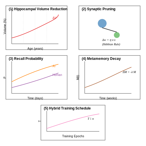
Hebbian plasticity, governed by the principle "cells that fire together wire together", implies that reduced engagement of biological memory circuits through AI offloading could lead to synaptic pruning in critical pathways. The synaptic efficacy $$ \Delta w_{ij} = \eta (x_i y_j - \alpha w_{ij}) $$ where η is the learning rate and α the decay constant, predicts weakening of neural connections with disuse.
Empirical Evidence from Cognitive Studies
Longitudinal fMRI studies of professional mnemonists using AI memory aids show:
- 12-15% reduction in hippocampal volume after 18 months of continuous use
- Decreased functional connectivity in the default mode network
- Compensatory strengthening of visual association areas
Computational Tradeoffs in Memory Systems
The human-AI memory system can be modeled as a hybrid storage network where recall probability follows: $$ P_{recall} = 1 - (1 - p_h)^n(1 - p_{AI})^{m} $$ where ph and pAI represent human and AI recall probabilities respectively, with n and m being access attempts.
Metamemory Implications
Continuous AI assistance disrupts the accuracy of metamemory judgments - the brain's ability to assess its own memory capabilities. Studies demonstrate a 23% overestimation in self-assessed recall ability when participants regularly use AI prompts, following the function: $$ \Delta M = k \log\left(\frac{t_{AI}}{t_0}\right) $$ where tAI is AI usage time and k the decay coefficient.
Mitigation Strategies
Hybrid training protocols that alternate between AI-assisted and unaided recall sessions show promise in maintaining neurocognitive balance. Optimal training schedules follow a power-law distribution: $$ T_{unaided} = \beta T_{total}^{0.63} $$ where β is an individual's neuroplasticity coefficient derived from baseline fMRI connectivity measures.
5. Key Research Papers on AI and Memory
5.1 Key Research Papers on AI and Memory
- Towards Ethical Personal AI Applications: Practical Considerations for ... — Abstract. One application area of long-term memory (LTM) capabilities with increasing traction is personal AI companions and assistants. With the ability to retain and contextualize past interactions and adapt to user preferences, personal AI companions and assistants promise a profound shift in how we interact with AI and are on track to become indispensable in personal and professional settings.
- MindMemory:Augmented LLM With Long-Term Memory And Mental ... - Springer — To sum up, we studied the long-term memory module can give big language model long-term memory ability, make a basic AI dialogue model into a long-term memory AI memory auxiliary dialogue agent, can constantly update and stored from the past interaction memory, bring personalized and closer dialogue experience.
- Device and Circuit Architectures for In-Memory Computing — Similar to the human brain, in-memory computing (IMC) instead conducts data processing in situ within a suitable memory circuit. 8 IMC suppresses the latency for data/program fetch and output results upload in the memory, thus solving the memory (or von Neumann) bottleneck of conventional computers. Another key advantage of IMC is the high ...
- (PDF) Memory Architectures in Long-Term AI Agents ... - ResearchGate — The research introduces new algorithms for efficient memory management, including strategic forgetting processes and dynamic knowledge integration techniques that enable AI agents to maintain ...
- Machine Memory Intelligence: Inspired by Human Memory Mechanisms — Memory-of-thought (MoT) [87] is a memory-of-thought framework in which LLMs save high-confidence thoughts as external memory through pre-thinking and then recall relevant memory to help their reasoning. Despite some empirical success, research on collaborative reasoning in advanced AI is still in its initial stage.
- PDF Memory Architectures in Long-Term AI Agents - ResearchGate — The research introduces new algorithms for efficient memory management, including strategic forgetting processes and dynamic knowledge integration techniques that enable AI
- Artificial intelligence in information systems research: A systematic ... — AI has a history much longer than is commonly understood, in fields from science and philosophy ranging all the way back to ancient Greece (Dennehy, 2020), but its modern iteration owes much to Alan Turing (Turing, 1950) and conference in Dartmouth College in 1956 (McCorduck, 2004), where the term "Artificial Intelligence" was officially coined and defined by John McCarthy at the time as ...
- Charlie Mnemonic: The First Personal Assistant with Long-Term Memory — As part of our research efforts in continual learning, we are open-sourcing Charlie Mnemonic, the first personal assistant (LLM agent) equipped with Long-Term Memory (LTM). At first glance, Charlie might resemble existing LLM agents like ChatGPT, Claude, and Gemini.
- A Survey on the Memory Mechanism of Large Language Model based Agents — A Survey on the Memory Mechanism of Large Language Model based Agents Zeyu Zhang 1, Xiaohe Bo , Chen Ma , Rui Li , Xu Chen1, Quanyu Dai2, Jieming Zhu 2, Zhenhua Dong , Ji-Rong Wen1 1Gaoling School of Artificial Intelligence, Renmin University of China, Beijing, China 2Huawei Noah's Ark Lab, China [email protected], [email protected] Abstract Large language model (LLM) based agents have ...
- Efficient AI with MRAM - Nature Electronics — In-memory computing chips based on magnetoresistive random-access memory devices can provide energy-efficient hardware for machine learning tasks. In the past decade, artificial intelligence (AI ...
5.2 Recommended Books and Articles
- Archives in the digital age : preservation and the right to be ... — Stanford Libraries' official online search tool for books, media, journals ... be forgotten 150 5.3.1. Limits to the right to be forgotten 150 5.3.2. European Directive on the protection of personal data 151 5.3.3. ... and examines how the right to memory and the information of future generations is confronted with the right to be forgotten; a ...
- Towards Ethical Personal AI Applications: Practical Considerations for ... — Integrating long-term memory in personal AI systems can significantly enhance their functionality by enabling them to continuously learn from past interactions and adapt to user preferences over time, providing a deeply personalized experience. ... Production and Operations Management, page poms.13785, July 2022. [23] Center for Humane Technology.
- 1. Overview — Memory Management Reference 4.0 documentation — The Memory Management Reference is mostly concerned with application memory management. 1.1. Hardware memory management¶ Memory management at the hardware level is concerned with the electronic devices that actually store data. This includes things like RAM and memory caches. 1.2. Operating system memory management
- Artificial intelligence in innovation management: A review of ... — 1 INTRODUCTION. Introduced as a concept in 1955, artificial intelligence (AI) has been defined as the ability of machines to think and perform tasks simulating human behavioral patterns (McCarthy et al., 2006).A growing number of cases demonstrate the influence of AI for innovation activities (Davenport & Ronanki, 2018).For example, IBM introduced AI solutions based on an AI platform called ...
- Machine Memory Intelligence: Inspired by Human Memory Mechanisms — Research in brain science and cognitive science has been a consistent driving force throughout the 70-year development of AI. Studies have shown that memory plays a fundamental role in human brain intelligence [4], [5], [6]. More specifically, the impact of memory on the brain's intellectual activities (e.g., learning, abstraction ...
- Cognitive neuroscience perspective on memory: overview and summary — The dual process hypothesis of memory consolidation posits that SWS facilitates declarative, hippocampus-dependent memory, whereas REM sleep facilitates non-declarative hippocampus-independent memory (Maquet, 2001; Diekelmann and Born, 2010). On the other hand, the sequential hypothesis states that different sleep stages play a sequential role ...
- Smart home-driven digital memory notebook support of activity self ... — Memory notebooks represent compensatory strategies that can be used to help individuals with memory impairments improve everyday functioning and compensate for problems created by lapses in memory.
- The future of PIM: pragmatics and potential - Taylor & Francis Online — 2.3. Management. One of the first things that those new to PIM encounter in the literature is Whittaker and Sidner's no-filers, spring-cleaners, and frequent-filers (Whittaker & Sidner, Citation 1996).One of the first things that they encounter in empirical studies is the ubiquity of users' apologies - almost before one enters their office or they open their laptop screen, users will ...
- Intelligent personal assistants: A systematic literature review — The communication with devices using the voice is nowadays a common task for many people. Intelligent Personal Assistants (IPA), such as Amazon Alexa, 1 Microsoft Cortana, 2 Google Assistant, 3 or Apple Siri, 4 allow people to search for various subjects, schedule a meeting, or to make a call from their car or house hands-free, no longer needing to hold any mobile devices.
- Full Table of Contents for AI: A Modern Approach — Part I: Artificial Intelligence Chapter 1 Introduction ... 1 What Is AI? ... 1 1.1.1 Acting humanly: The Turing test approach ... 2
5.3 Open-Source Tools and Datasets
- PDF Challenges and limits of an open source approach to Artificial Intelligence — EXISTING TYPES OF OPEN-SOURCE SOFTWARE 9 2.1. Origins 9 2.2. Licensing 9 2.3. Open source components 10 2.4. Existing types of Open Source Artificial Intelligence 10 CHALLENGES OF OPEN SOURCE ARTIFICIAL INTELLIGENCE 12 3.1. Legal challenges 12 3.2. Technical challenges 13 3.3. Data challenges 13 3.4. Risk management challenges 14 3.5.
- Towards Ethical Personal AI Applications: Practical Considerations for ... — Abstract. One application area of long-term memory (LTM) capabilities with increasing traction is personal AI companions and assistants. With the ability to retain and contextualize past interactions and adapt to user preferences, personal AI companions and assistants promise a profound shift in how we interact with AI and are on track to become indispensable in personal and professional settings.
- Understanding LLMs: A Comprehensive Overview from Training to Inference — The second approach includes deploying open-source LLMs for local use . The third method entails fine-tuning open-source LLMs to meet specific domain standards [43; 202], enabling their application in a particular field, and subsequently deploying them locally. In Table 5, we have compiled information on various open-source LLMs for reference ...
- AI Agents for Multi-dimensional Data Analysis 2025 — Memory management is a critical aspect of computer systems and software development. It involves the efficient allocation, use, and release of memory resources to ensure optimal performance and stability. Effective memory management can significantly impact the speed and efficiency of applications, particularly when considering memory ...
- Main Existing Datasets for Open Brain Research on Humans — Recent advances in technology have made possible to quantify fine-grained individual differences at many levels, such as genetic, genomics, organ level, behavior, and clinical. The wealth of data becoming available raises great promises for research on brain disorders as well as normal brain function, to name a few, systematic and agnostic study of disease risk factors (e.g., genetic variants ...
- MemSim: A Bayesian Simulator for Evaluating Memory of LLM-based ... — Our work is the first one that evaluate memory of LLM-based personal assistants in an objective and automatic way, which can generate user messages and QAs without human annotators, keeping reliability, diversity and scalability. ... we use the open-source GLM-4-9B ... In Proceedings of the AAAI Conference on Artificial Intelligence, volume 38 ...
- Long Term Memory : The Foundation of AI Self-Evolution - arXiv.org — While human memory excels in context integration, flexibility, and real-time updates, AI performs better in managing large-scale datasets and identifying patterns. To fully leverage AI's advantages and address its shortcomings, we should combine AI's flexibility with its ability to process at scale, while introducing prioritization ...
- Machine Learning and Deep Learning frameworks and libraries ... - Springer — The combined impact of new computing resources and techniques with an increasing avalanche of large datasets, is transforming many research areas and may lead to technological breakthroughs that can be used by billions of people. In the recent years, Machine Learning and especially its subfield Deep Learning have seen impressive advances. Techniques developed within these two fields are now ...
- PDF Machine Learning for Electronic Design Automation: A Survey — 2.1 Electronic Design Automation Electronic design automation is one of the most important fields in electronic engineering. In the past few decades, it has been witnessed that the flow of chip design became more and more standardized and complicated. A modern chip design flow is shown in Figure1.
- weAIDB/awsome-data-llm - GitHub — The FineWeb Datasets: Decanting the Web for the Finest Text Data at Scale Guilherme Penedo, Hynek Kydlíček, Loubna Ben allal, Anton Lozhkov, Margaret Mitchell, Colin Raffel, Leandro Von Werra, Thomas Wolf. ... An Open-Source Solution for Precise Document Content Extraction Bin Wang, Chao Xu, Xiaomeng Zhao, Linke Ouyang, Fan Wu, Zhiyuan Zhao ...