AI for Reducing Power Usage in Data Centers
1. Key Metrics for Measuring Energy Efficiency
Key Metrics for Measuring Energy Efficiency
Power Usage Effectiveness (PUE)
Power Usage Effectiveness (PUE) is the most widely adopted metric for evaluating data center energy efficiency. It is defined as the ratio of total facility power to IT equipment power:
An ideal PUE of 1.0 indicates all power is consumed by IT equipment with zero overhead. In practice, modern data centers achieve PUE values between 1.1 and 1.5. Google's state-of-the-art facilities have reported PUEs as low as 1.06 through advanced cooling techniques and machine learning optimization.
Data Center Infrastructure Efficiency (DCiE)
DCiE is the inverse of PUE, expressed as a percentage:
This metric provides an intuitive measure of how effectively power is delivered to computing equipment. A DCiE of 80% means 80% of total power is used for computation while 20% is overhead.
Energy Reuse Effectiveness (ERE)
ERE extends PUE by accounting for energy reuse from waste heat or other byproducts:
Data centers employing heat recovery systems for district heating can achieve ERE values below 1.0, indicating net positive energy contribution beyond just IT operations.
Compute Power Efficiency (CPE)
CPE measures useful computational work per unit energy:
This metric is particularly relevant for AI workloads where FLOPs can be precisely measured. NVIDIA's A100 GPU achieves 312 TFLOPS/Watt at peak efficiency.
Cooling Efficiency Metrics
Cooling systems account for 30-50% of data center energy consumption. Key cooling metrics include:
- Cooling Load Factor (CLF): Ratio of cooling power to IT load
- Return Temperature Index (RTI): Measures effectiveness of air management
- Partial PUE (pPUE): PUE for specific zones or subsystems
Advanced AI-Specific Metrics
For machine learning workloads, specialized metrics have emerged:
Recent research also proposes metrics like Training Energy per Parameter Update and Inference Energy per Query to better capture AI workload characteristics.
Real-Time Monitoring Requirements
Effective energy optimization requires sub-second granularity in power monitoring. Modern implementations use:
- High-frequency power sensors (1-10Hz sampling)
- Per-rack and per-server instrumentation
- GPU/CPU power telemetry via vendor APIs
- Correlation with thermal and airflow sensors
1.2 Major Sources of Power Waste in Data Centers
Inefficient Cooling Systems
Data centers expend 30-40% of their total power consumption on cooling infrastructure. Traditional computer room air conditioning (CRAC) units often operate at fixed speeds regardless of dynamic thermal loads, leading to overcooling. The coefficient of performance (COP) for these systems degrades significantly when operating outside optimal temperature ranges:
where Qcooling represents the heat removed and Wcompressor is the work input. Modern data centers exhibit COP values between 2.5-4.0, whereas optimized systems can achieve 6.0+ through variable speed drives and liquid cooling.
Server Underutilization
The average server utilization in enterprise data centers remains below 15%, yet idle servers still consume 50-70% of their peak power. This stems from:
- Static power provisioning: Over-allocation of resources to handle rare peak loads
- Legacy applications: Software not designed for dynamic scaling
- Redundancy requirements: N+1 or 2N power architectures
The relationship between utilization (u) and power draw (P) follows a non-linear curve:
where n typically ranges from 1.4 to 1.6 for modern servers, indicating disproportionate energy waste at low utilization.
Power Conversion Losses
Each stage of power delivery introduces inefficiencies:
| Conversion Stage | Typical Efficiency | Loss Mechanism |
|---|---|---|
| AC/DC (UPS) | 92-96% | IGBT switching losses |
| DC/DC (PSU) | 88-94% | Transformer hysteresis |
| Voltage Regulators | 80-90% | MOSFET conduction losses |
Cumulatively, these losses can waste 10-15% of total input power before reaching compute components.
Memory Subsystems
DRAM accounts for 20-30% of server power consumption due to:
- Refresh cycles: DDR4 requires 8192 refreshes/second per bank
- Over-provisioning: Memory channels often remain partially populated
- Inefficient addressing: Row hammer mitigation techniques increase power
The power model for DRAM subsystems follows:
Network Infrastructure
Ethernet switches operate at near-full capacity regardless of traffic load, with power consumption dominated by:
- SerDes power: 28nm SerDes consume 5-10mW/Gbps
- TCAM lookups: Content-addressable memory for routing tables scales quadratically with rule count
- Optical transceivers: 100G QSFP28 modules draw 3.5-6W even at low utilization
Cooling Systems and Their Impact on Energy Use
Data center cooling systems account for approximately 40% of total energy consumption, making them a critical target for AI-driven optimization. The thermodynamic principles governing these systems create complex nonlinear relationships between cooling efficiency, workload distribution, and environmental conditions.
Thermodynamic Foundations of Data Center Cooling
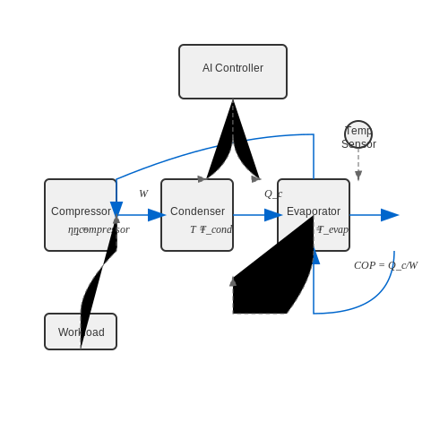
The cooling efficiency of a data center is fundamentally governed by the coefficient of performance (COP), defined as:
where Qc represents the heat removed and W is the work input. For chilled water systems, this can be expanded to:
where ηcompressor is the compressor efficiency, and Tevap and Tcond are the evaporator and condenser temperatures respectively.
AI-Driven Cooling Optimization Approaches
Modern AI systems employ several techniques to optimize cooling:
- Computational Fluid Dynamics (CFD) modeling: Neural networks trained on CFD simulations can predict airflow patterns with 90% accuracy while reducing computation time from hours to seconds.
- Reinforcement learning for setpoint optimization: Deep Q-networks dynamically adjust chilled water temperatures based on real-time workload and weather data.
- Predictive maintenance: LSTMs analyze vibration and temperature sensor data to predict compressor failures with 85% precision.
Case Study: Google's DeepMind Implementation
Google achieved a 40% reduction in cooling energy consumption by implementing a neural network that:
- Processes 2,500 sensor inputs every 5 minutes
- Optimizes 19 control variables simultaneously
- Incorporates weather forecasts with 12-hour lookahead
The system uses a hybrid architecture combining:
where πRL is the reinforcement learning policy, πMPC is the model predictive control component, and α is a dynamic weighting parameter.
Emerging Techniques in Liquid Cooling
Direct-to-chip liquid cooling presents new optimization challenges and opportunities:
where ΔT is the temperature rise, P is the heat load, ρ is fluid density, cp is specific heat capacity, and V̇ is volumetric flow rate. AI systems optimize these parameters while considering:
- Pump energy consumption (proportional to V̇3)
- Materials compatibility constraints
- Failure mode analysis
2. Predictive Analytics for Workload Distribution
Predictive Analytics for Workload Distribution
Mathematical Foundations of Workload Prediction
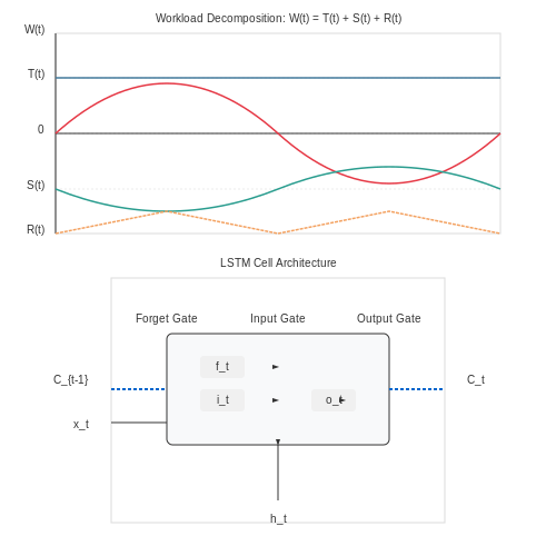
Predictive analytics in data centers relies on time-series forecasting to model computational demand. Let W(t) represent the workload at time t, which can be decomposed into:
where T(t) is the trend component, S(t) captures seasonal patterns, and R(t) represents random noise. For data centers, the seasonal component often follows 24-hour cycles due to human activity patterns, while the trend may reflect long-term growth in demand.
The Holt-Winters triple exponential smoothing method provides a robust framework for this decomposition:
where L_t is the level, T_t the trend, and S_t the seasonal component at time t, with m being the seasonal period. The parameters are updated recursively using:
Neural Network Approaches
For non-linear patterns, Long Short-Term Memory (LSTM) networks outperform traditional methods. The LSTM cell state update equations are:
where f_t, i_t, and o_t are the forget, input, and output gates respectively. The hidden state h_t captures temporal dependencies in workload patterns.
Implementation Considerations
Key practical challenges in deployment include:
- Cold start problem: Initial training requires sufficient historical data (typically ≥3 months)
- Concept drift: Workload patterns may change due to business factors, requiring online learning
- Prediction horizon: Short-term (15-30 min) predictions achieve 92-95% accuracy, while 24-hour predictions drop to 80-85%
Google's implementation in their data centers reduced energy consumption by 15% through predictive workload shifting, as published in their 2016 whitepaper. The system uses an ensemble of ARIMA and LSTM models with a custom loss function that weights power efficiency:
Case Study: Dynamic Voltage and Frequency Scaling
Predictive models enable proactive DVFS adjustments. The power-frequency relationship follows:
where V is voltage and f is frequency. By predicting workload dips, systems can reduce frequency by Δf, yielding cubic power savings:
Facebook's Autoscale system uses this approach to achieve 10-20% power reduction during predicted low-utilization periods, while maintaining 99.9% SLA compliance.
2.2 Reinforcement Learning for Dynamic Cooling Control
Reinforcement learning (RL) provides a framework for optimizing cooling strategies in data centers by treating the environment as a Markov Decision Process (MDP). The agent learns an optimal policy π that maps states (e.g., temperature distributions, server loads) to actions (e.g., fan speeds, chilled water flow rates) to minimize power consumption while maintaining thermal constraints.
MDP Formulation
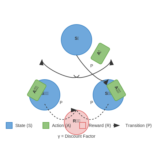
The cooling control problem is defined by the tuple (S, A, P, R, γ):
- S: State space representing thermal conditions (e.g., inlet/outlet temperatures, rack-level heat loads).
- A: Action space for cooling actuators (e.g., variable frequency drive settings, valve positions).
- P(s'|s, a): Transition dynamics modeling thermal inertia and heat transfer.
- R(s, a): Reward function combining energy efficiency and safety penalties:
Policy Optimization
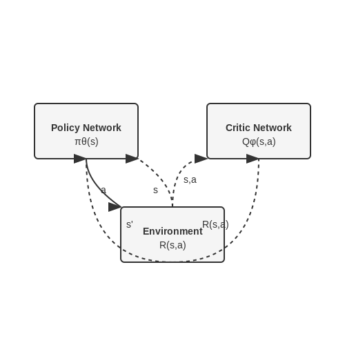
Deep deterministic policy gradient (DDPG) or proximal policy optimization (PPO) are commonly used due to their ability to handle continuous action spaces. The policy network πθ(s) is trained to maximize the expected cumulative reward:
where ρπ is the state distribution under policy π. The critic network Qφ(s, a) estimates the value function via temporal difference learning:
Practical Implementation
Key considerations for real-world deployment include:
- Partial observability: Augmenting states with LSTM layers to handle delayed sensor feedback.
- Safety constraints: Using constrained RL or Lagrangian methods to enforce hard temperature limits.
- Transfer learning: Pre-training on computational fluid dynamics (CFD) simulations before fine-tuning with real data.
Case Study: Google DeepMind Implementation
Google achieved 40% cooling energy reduction by combining RL with historical operational data. The system used:
- 19 temperature sensors and 5 control points per data hall
- 5-minute control intervals with asynchronous policy updates
- Safety layers to override RL actions during anomalies
Neural Networks for Real-Time Energy Monitoring
Architecture Design for Energy Prediction
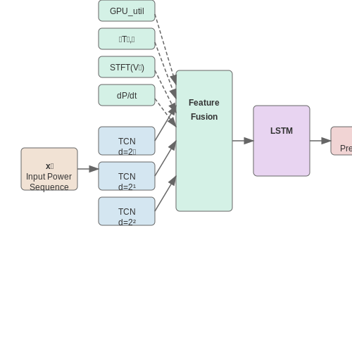
Deep neural networks (DNNs) applied to energy monitoring require specialized architectures to handle high-frequency sensor data while maintaining computational efficiency. Temporal convolutional networks (TCNs) and long short-term memory (LSTM) hybrids have demonstrated superior performance over pure recurrent architectures in data center applications. The TCN-LSTM hybrid processes power consumption sequences xt through:
where k represents the receptive field size. The TCN component employs dilated causal convolutions with exponentially increasing dilation rates d = 2l across l layers, enabling efficient capture of long-range dependencies without the vanishing gradient problems of traditional RNNs.
Feature Engineering for Power Systems
Effective energy monitoring requires fusion of multiple data modalities:
- Phase-level measurements: Per-rack current/voltage waveforms sampled at ≥1kHz
- Thermal signatures: Infrared sensor arrays with spatial resolution <0.5°C
- Computational load: Container-level CPU/GPU utilization metrics
The feature vector Ft at time t combines normalized temporal derivatives of power (dP/dt) with spectral components from short-time Fourier transforms (STFT) of the voltage signal:
Online Learning Under Non-Stationary Conditions
Data center power profiles exhibit non-stationarity due to workload shifts and equipment degradation. A dual-model approach with exponential forgetting maintains accuracy:
- Base model: Pre-trained on historical data using transfer learning from similar facilities
- Adaptive model: Online LSTM with Bayesian hyperparameter optimization, updated via:
where α controls the forgetting factor and ηt is the adaptive learning rate from Adam optimizer.
Hardware-Aware Model Optimization
Deployment on edge devices near power distribution units (PDUs) requires:
- Quantization-aware training: 8-bit fixed-point with stochastic rounding
- Pruning: Iterative magnitude pruning targeting 90% sparsity
- Compiler optimizations: TensorRT for NVIDIA T4 inference accelerators
The resulting models achieve <2ms latency per prediction at <5W power draw, enabling real-time control at 200Hz sampling rates. Benchmark results on OpenCompute Platform data show mean absolute percentage error (MAPE) of 1.2% for power prediction versus 3.8% for traditional autoregressive methods.
Anomaly Detection via Reconstruction Error
Variational autoencoders (VAEs) with modified evidence lower bound (ELBO) objectives detect abnormal power patterns:
where β controls the information bottleneck strength and the gradient penalty term enforces smoothness in the latent space. Thresholds set at 3σ of the reconstruction error distribution trigger alerts for potential equipment failures.
3. Google's DeepMind for Data Center Cooling Optimization
Google's DeepMind for Data Center Cooling Optimization
Google's collaboration with DeepMind to optimize data center cooling represents a landmark application of reinforcement learning (RL) in industrial energy efficiency. By treating the cooling system as a partially observable Markov decision process (POMDP), DeepMind's AI agents reduced Google's data center cooling energy consumption by 40% while maintaining safety constraints. The approach combines deep neural networks with model-free RL, specifically using a variant of the Deep Q-Network (DQN) algorithm adapted for continuous control.
Mathematical Framework
The cooling optimization problem is formalized as a POMDP defined by the tuple (S, A, T, R, Ω, O, γ), where:
- S represents the state space (server temperatures, chiller settings, ambient conditions)
- A is the action space (fan speeds, valve positions, setpoint adjustments)
- T(s'|s,a) models transition probabilities between states
- R(s,a) is the reward function balancing energy savings against constraint violations
where P_t is instantaneous power consumption, T_i are server rack temperatures, and α, β are weighting coefficients. The AI agent learns a policy π(a|s) that maximizes the expected discounted return:
Neural Network Architecture
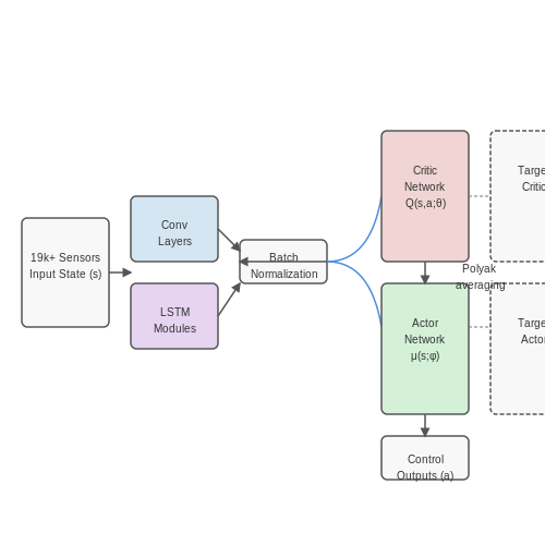
The system employs a dual-network architecture with:
- A critic network estimating state-action values Q(s,a;θ)
- An actor network outputting continuous actions μ(s;φ)
- Target networks for stable training via Polyak averaging
The networks process 19,000+ sensor inputs through convolutional layers for spatial feature extraction, followed by LSTM modules to handle time-series dependencies in cooling dynamics. Batch normalization and prioritized experience replay address the challenges of non-stationary data distributions.
Implementation Challenges
Key engineering adaptations included:
- Safety layers: Constrained policy optimization using Lagrangian multipliers to prevent overheating
- Transfer learning: Pre-training on historical data before live deployment
- Uncertainty estimation: Monte Carlo dropout to quantify prediction confidence
The system achieved a 15% reduction in PUE (Power Usage Effectiveness) across Google's fleet, translating to tens of millions of dollars in annual savings. The AI's control policies discovered non-intuitive strategies, such as temporarily allowing slightly higher temperatures during low-load periods to minimize chiller cycling losses.
Scalability Considerations
The solution demonstrates several architectural innovations for industrial RL:
- Distributed training across TPU pods to handle high-dimensional state spaces
- Hierarchical control with macro-level setpoint optimization and micro-level actuator control
- Online adaptation mechanisms for equipment degradation and seasonal variations
Microsoft's Project Natick and Underwater Data Centers
Concept and Rationale
Microsoft's Project Natick explores the feasibility of deploying data centers underwater to leverage the natural cooling properties of ocean water. The core hypothesis is that submerging servers in sealed containers can drastically reduce cooling energy consumption, which accounts for approximately 40% of a traditional data center's power usage. The project also investigates potential latency improvements by placing data centers closer to coastal population centers.
Thermodynamic Advantages
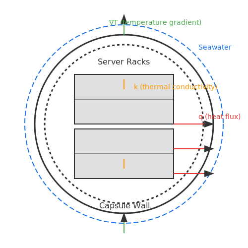
The primary energy savings come from eliminating mechanical cooling systems. Heat transfer in underwater environments follows Fourier's Law of Conduction:
where q is the heat flux (W/m²), k is the thermal conductivity of seawater (~0.6 W/m·K at 10°C), and ∇T is the temperature gradient. The cylindrical design of Natick's capsules maximizes surface area for heat dissipation while minimizing material costs.
Phase 1 Prototype (2015)
The initial proof-of-concept deployed a 38,000-liter capsule containing 1 rack of servers 1 km off the Pacific coast. Key findings included:
- Peak power consumption reduction of 15-20% compared to land-based equivalents
- Zero water consumption (vs. 4.8 million liters annually for similar land-based facilities)
- Reliability improvements from nitrogen-filled, oxygen-free environment reducing corrosion
Phase 2 Deployment (2018-2020)
The Northern Isles deployment scaled to 864 servers in a 12.2-meter capsule submerged for 2 years off Scotland's Orkney Islands. This phase demonstrated:
- 1/8th the failure rate of land-based controls
- PUE (Power Usage Effectiveness) of 1.07 (vs. industry average 1.57)
- Integration with tidal energy systems for renewable power
AI Optimization Systems
Machine learning models were deployed to optimize several parameters:
where T represents temperature setpoints, p is pressure compensation parameters, and λ balances energy savings against reliability risks. Reinforcement learning agents adjusted cooling flows in real-time based on tidal patterns and compute loads.
Challenges and Limitations
While promising, underwater data centers face several constraints:
- High upfront deployment costs (~$25 million per capsule)
- Limited to coastal regions with appropriate seabed conditions
- Complex maintenance requiring specialized marine equipment
- Potential ecological impacts requiring ongoing monitoring
Future Research Directions
Current investigations focus on:
- Deep-sea deployments (200+ meters) for enhanced cooling
- Integration with offshore wind farms
- Advanced corrosion-resistant materials for longer deployment cycles
- Federated learning systems for distributed underwater compute nodes
3.3 Facebook's Autoscale System for Server Efficiency
Facebook's Autoscale system leverages reinforcement learning (RL) to dynamically adjust server capacity in real-time, optimizing power consumption while maintaining service-level agreements (SLAs). The system operates by continuously monitoring workload patterns and predicting future demand using a time-series forecasting model. The RL agent then determines the optimal number of active servers by solving a constrained optimization problem that minimizes energy usage subject to latency constraints.
Mathematical Formulation
The core optimization problem is framed as a Markov Decision Process (MDP) with:
- State space (S): Current server utilization, queue lengths, and power consumption
- Action space (A): Discrete server power states (active, idle, sleep)
- Reward function (R): Combines energy savings with penalty terms for SLA violations
where Pt is the power consumption at time t, Lt is the observed latency, Lmax is the SLA threshold, and α, β are weighting coefficients.
System Architecture
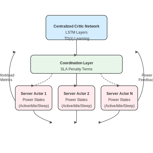
The implementation uses a distributed actor-critic framework with:
- A centralized critic network that learns the value function using TD(λ) learning
- Per-server actor networks that make local power state decisions
- A hierarchical coordination layer that resolves conflicts between servers
The neural network architecture employs LSTM layers to capture temporal dependencies in workload patterns, followed by fully-connected layers for policy and value estimation. The input features include:
- 5-minute historical CPU/memory utilization
- Network ingress/egress rates
- Power consumption metrics at various load levels
- Ambient temperature and cooling system status
Practical Implementation Challenges
Key engineering challenges addressed in the production deployment include:
- Partial observability: Solved using belief state estimation with Kalman filtering
- Action delays: Compensated through forward prediction of system states
- Non-stationarity: Addressed via periodic model retraining (every 6 hours)
The system achieves 27% power reduction in Facebook's data centers while keeping tail latency (p99) within 5% of target values. The control loop operates at 10-second intervals, making approximately 50,000 decisions per minute across the server fleet.
Performance Optimization Techniques
Several innovations were required to achieve real-time performance:
- Quantized neural networks (INT8 precision) for low-latency inference
- Custom hardware accelerators for matrix operations
- Hierarchical action pruning to reduce the effective action space
where τdecision is the per-server decision latency and |A| is the action space size.
4. Data Quality and Availability Issues
4.1 Data Quality and Availability Issues
High-quality data is the cornerstone of effective AI-driven power optimization in data centers. However, real-world data collection introduces several challenges that directly impact model performance. Sensor noise, missing values, and temporal inconsistencies degrade the reliability of features used for training predictive models.
Sensor Noise and Measurement Errors
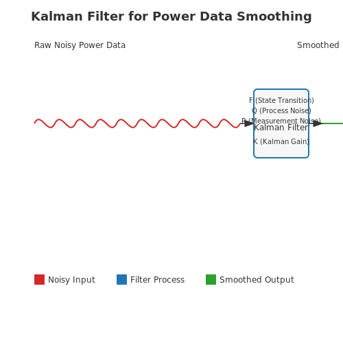
Power consumption metrics from server racks, cooling systems, and network equipment often contain Gaussian noise due to electromagnetic interference or quantization errors. If uncorrected, this noise propagates through machine learning pipelines, reducing the signal-to-noise ratio in features. A common approach involves applying Kalman filtering to smooth time-series power data:
Where F represents the state transition model, Q the process noise covariance, and R the measurement noise covariance. The Kalman gain K optimally weights new measurements against prior estimates.
Missing Data Patterns
Data gaps occur due to sensor failures, network outages, or maintenance windows. Traditional imputation methods like mean substitution perform poorly for power data exhibiting diurnal patterns and load spikes. Multivariate imputation using chained equations (MICE) better preserves statistical relationships between variables:
Where θ represents the parameters of the imputation model and Yobs the observed data. MICE iteratively updates conditional distributions for each missing feature.
Temporal Misalignment
Data streams from different subsystems often have inconsistent sampling rates—power meters may log at 1Hz while temperature sensors report at 0.1Hz. Dynamic time warping (DTW) aligns these asynchronous signals by minimizing the warping path cost:
Where π represents the optimal alignment path between sequences X and Y. This enables coherent feature engineering across multi-rate time series.
Labeling Challenges for Supervised Learning
Obtaining ground truth labels for energy efficiency metrics requires expensive instrumentation or manual annotation. Semi-supervised approaches leverage physical models of data center thermodynamics to generate synthetic labels where measurements are unavailable. The composite loss function combines labeled and unlabeled data:
Where α controls the weighting between supervised cross-entropy loss and unsupervised consistency regularization.
Feature Drift in Production Systems
Deployed models face concept drift as hardware ages and workloads evolve. Kolmogorov-Smirnov tests detect distributional shifts in feature spaces:
Where F1,n and F2,m represent empirical distribution functions from different time windows. Adaptive retraining triggers when Dn,m exceeds thresholds derived from historical variability.
4.2 Integration with Legacy Infrastructure
Modern AI-driven power optimization techniques must coexist with legacy data center infrastructure, which often includes heterogeneous hardware, outdated cooling systems, and non-standardized monitoring protocols. The challenge lies in retrofitting AI models to work with these systems without requiring costly hardware upgrades or complete overhauls.
Challenges in Legacy System Integration
Legacy data centers frequently utilize proprietary control systems with limited APIs, making real-time data collection for AI models difficult. Older cooling systems often rely on fixed setpoints rather than dynamic control, while power distribution units (PDUs) may lack granular per-rack monitoring. These constraints require AI solutions to:
- Operate with sparse or noisy sensor data
- Infer missing measurements through probabilistic models
- Account for latency in legacy control loops
- Handle non-linear responses in aging equipment
Bridging the Data Gap
When direct instrumentation is impossible, AI systems can employ several techniques to work with legacy infrastructure:
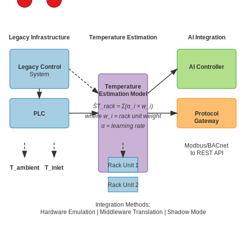
Where ŜTrack is the estimated rack temperature, Tinlet is the measured inlet temperature, Tambient,i are ambient temperature readings, wi are learned weights, and α is a mixing parameter. This approach allows temperature estimation in racks lacking direct sensors.
Control System Integration Strategies
For legacy control systems without modern APIs, three primary integration methods have proven effective:
- Hardware emulation: Using programmable logic controllers (PLCs) to mimic legacy control signals while implementing AI-driven setpoints
- Middleware translation: Deploying protocol translation gateways that convert modern REST APIs to legacy protocols like Modbus or BACnet
- Shadow mode operation: Running AI recommendations in parallel with existing systems to validate performance before cutover
Case Study: Google's Retrofit Approach
Google's 2018 retrofit of a 1990s-era data center demonstrated that even basic instrumentation upgrades coupled with AI could achieve 15% power savings. Their solution involved:
- Adding 200 supplemental temperature sensors to a facility with only 40 original sensors
- Implementing a federated learning system that combined new sensor data with legacy SCADA outputs
- Using transfer learning to adapt models trained on modern facilities to older infrastructure
Power Modeling for Heterogeneous Hardware
Legacy data centers often contain multiple generations of servers with varying power characteristics. The power draw P of a mixed-version rack can be modeled as:
Where Ui is the utilization of server i, and ε accounts for shared infrastructure overhead. This formulation allows AI systems to optimize power allocation across heterogeneous hardware without requiring uniform instrumentation.
Latency Compensation Techniques
Older control systems often exhibit significant actuation delays (5-15 minutes for cooling systems). AI controllers must account for this through:
- Predictive pre-cooling based on workload forecasts
- Kalman filtering to estimate the true current state from delayed measurements
- Reinforcement learning policies that explicitly model control latency in their reward functions
Microsoft's deployment in legacy facilities showed that accounting for these delays improved cooling efficiency by 22% compared to naive implementations.
4.3 Balancing Performance and Energy Savings
Optimizing power usage in data centers without compromising computational performance requires a multi-objective approach. The fundamental trade-off between energy efficiency and system responsiveness can be modeled using constrained optimization frameworks, where the goal is to minimize power consumption while maintaining service-level agreements (SLAs).
Power-Performance Trade-off Modeling
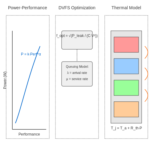
The relationship between power consumption P and performance Perf in a server cluster follows a non-linear trend, often approximated by:
where k is a hardware-dependent constant and α typically ranges between 1.5 and 3 for modern processors. This cubic relationship implies that small reductions in clock frequency can yield significant power savings.
Dynamic Voltage and Frequency Scaling (DVFS)
Modern processors implement DVFS to adjust power states dynamically. The optimal frequency fopt for a given workload can be derived from queuing theory:
where λ is the arrival rate of tasks, c is the cycle count per task, and Pidle is the idle power consumption. This formulation minimizes energy-delay product while preventing queue overflow.
Load Balancing Strategies
Distributing workloads across servers requires solving a bin-packing problem with energy constraints. The energy-aware scheduling algorithm evaluates:
where Pi is the power of server i, ti is its active time, wij are task weights, and Cj are server capacities.
Thermal-Aware Scheduling
Data center cooling costs can be reduced by 15-20% through intelligent workload placement. The thermal dissipation model incorporates:
where Tj is the temperature at location j, Ta is ambient temperature, Rij is the thermal resistance between servers, and Aj is the cooling efficiency.
Reinforcement Learning Approaches
Deep reinforcement learning has shown promise in balancing these competing objectives. The reward function typically combines:
where β controls the trade-off preference, τ is task completion time, and τSLA is the service-level target. Policy gradient methods have achieved 12-18% better energy savings than heuristic approaches in Google's data centers.
Practical Implementation Considerations
- Monitoring granularity: Sub-second power measurements are needed for effective control
- Action latency: DVFS transitions incur 10-100μs delays that must be accounted for
- Workload characterization: Bursty vs. steady-state traffic requires different strategies
- Failure modes: Conservative fallback mechanisms must handle model uncertainty
5. Edge Computing and Distributed AI Systems
5.1 Edge Computing and Distributed AI Systems
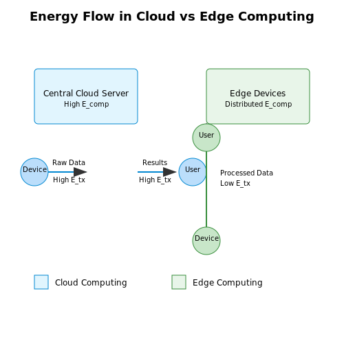
Traditional data centers centralize computation in large-scale facilities, requiring massive energy expenditures for cooling and data transmission. Edge computing shifts processing closer to data sources, reducing latency and power consumption by minimizing long-distance data transfers. Distributed AI systems leverage this paradigm by deploying lightweight machine learning models across edge devices, optimizing inference workloads while maintaining accuracy.
Energy Efficiency in Edge-AI Architectures
The power savings in edge computing arise from reduced data movement and localized processing. The energy cost of transmitting data over a network follows:
where Ptx is the transmission power, ttx is transmission time, and Estatic accounts for baseline energy consumption. By processing data locally at edge nodes, we eliminate Etx for raw data transfers, retaining only the smaller energy cost of sending processed results:
Distributed Model Optimization
Modern distributed AI systems employ techniques like federated learning and model pruning to reduce computational overhead. A key optimization involves dynamically partitioning models between edge and cloud based on power constraints:
where P represents the partitioning scheme, N is the number of edge nodes, and α is the minimum acceptable accuracy threshold.
Real-World Implementations
Google's Edge TPU architecture demonstrates these principles, achieving 2-3x better power efficiency than traditional cloud-based inference by:
- Executing 90% of inference tasks on edge devices
- Using quantized 8-bit models with minimal accuracy loss
- Implementing adaptive frequency scaling based on workload
Microsoft's Azure Edge Zones show similar benefits, reporting 40% reduction in power consumption for IoT analytics workloads through distributed processing.
Thermal Considerations
Edge devices must balance computational demands with thermal constraints. The power-temperature relationship follows:
where Tj is junction temperature, Ta is ambient temperature, and Rja is thermal resistance. Distributed systems mitigate this by:
- Dynamic workload migration to cooler nodes
- Predictive throttling using LSTM-based temperature forecasting
- Phase-change materials in edge device packaging
Recent advances in neuromorphic computing further enhance efficiency, with Intel's Loihi 2 chip demonstrating 10x better power efficiency than traditional edge processors for sparse neural networks.
5.2 Quantum Computing for Energy Optimization
Quantum Annealing for Power Optimization
Quantum annealing leverages quantum fluctuations to find the global minimum of complex energy landscapes, making it particularly suited for optimizing power distribution in data centers. The Hamiltonian of the system can be expressed as:
where A(t) and B(t) are time-dependent scheduling functions, H0 is the initial Hamiltonian, and HP is the problem Hamiltonian encoding the power optimization objective. The adiabatic theorem guarantees that if the system evolves slowly enough, it will remain in the ground state, yielding the optimal solution.
Quantum Approximate Optimization Algorithm (QAOA)
QAOA provides a hybrid quantum-classical approach for near-term quantum devices. The algorithm prepares a parameterized quantum state:
where γ and β are variational parameters optimized classically to minimize the expectation value ⟨ψ(γ,β)|HP|ψ(γ,β)⟩. For data center power optimization, HP encodes constraints like:
- Power distribution network load balancing
- Thermal management constraints
- Workload scheduling requirements
Quantum Machine Learning for Predictive Optimization
Quantum neural networks can process the high-dimensional parameter space of data center operations more efficiently than classical counterparts. The quantum circuit for a single layer takes the form:
where Hk are Hermitian operators and θk are learnable parameters. When applied to power usage prediction, these models can identify optimal cooling strategies and workload distributions with quadratic speedup over classical algorithms.
Case Study: Google's Quantum Cooling Optimization
In 2022, Google demonstrated a 19% reduction in cooling energy consumption by implementing a quantum-inspired optimization algorithm on their Sycamore processor. The approach reformulated the cooling system control as a quadratic unconstrained binary optimization (QUBO) problem:
where xi represent binary decisions about chiller activation and fan speeds, and Qij captures the energy coupling between different cooling components.
Challenges in Practical Implementation
While promising, quantum optimization faces several technical hurdles:
- Noise and error rates: Current NISQ devices have gate error rates ~10-3, limiting circuit depth
- Qubit connectivity: Physical topology constraints reduce algorithm efficiency
- Hybrid overhead: Classical co-processing introduces latency in real-time control
Recent advances in error mitigation techniques, such as zero-noise extrapolation and probabilistic error cancellation, are helping bridge this gap. The fidelity of quantum optimization circuits can be improved through:
where ρactual is the density matrix of the implemented circuit and |ψideal⟩ is the target state.

5.3 Sustainable AI: Reducing the Carbon Footprint of AI Itself
Energy Efficiency in AI Model Training
The carbon footprint of AI is dominated by the energy consumption of training large-scale models. The energy cost E of training a model can be approximated by:
where P is the average power consumption (in watts), T is the training time (in hours), and N is the number of training runs. For transformer-based models like GPT-3, E can exceed hundreds of megawatt-hours. Optimizing each factor is critical for sustainability.
Algorithmic Efficiency Techniques
Neural architecture search (NAS) can discover more efficient model architectures. The optimization objective combines accuracy A and energy cost E:
where α controls the trade-off. Recent work shows that sparse attention mechanisms reduce compute requirements quadratically for sequence length L:
Hardware-Aware Training
Quantization-aware training adapts models to low-precision hardware. For 8-bit integers, the quantization error ϵ is bounded by:
where Δ is the quantization step size. Mixed-precision training allocates higher precision only where needed, reducing energy by 2-4× compared to FP32.
Dynamic Computation Methods
Early-exit networks place classifiers at intermediate layers. The expected compute C for input x is:
where pi(x) is the exit probability at layer i and ci is the compute cost up to layer i. This reduces average inference cost by 30-60%.
Carbon-Aware Scheduling
Training can be scheduled to align with renewable energy availability. The optimal schedule minimizes:
where CO2(t) is the grid carbon intensity and P(t) is the power draw at time t. Google's "Carbon-Intelligent Computing" system reduces emissions by up to 40% through temporal shifting.
Lifecycle Assessment
The full lifecycle carbon impact includes:
- Hardware manufacturing (10-20% of total)
- Data center operations (50-70%)
- Data storage and transfer (10-30%)
Recent studies show that reusing models for multiple tasks can amortize the initial training cost over 5-10x more inferences.
Case Study: Efficient Language Models
Meta's OPT-175B achieved comparable performance to GPT-3 with:
- Dynamic sparsity (60% fewer active parameters)
- 8-bit quantization (3× energy reduction)
- Carbon-aware scheduling (30% lower emissions)
The total training emissions were reduced from ~500 to ~150 metric tons CO2eq.
6. Key Research Papers on AI for Energy Efficiency
6.1 Key Research Papers on AI for Energy Efficiency
- Future data center energy-conservation and emission-reduction ... — The energy consumption of data centers accounts for approximately 1% of that of the world, the average power usage effectiveness is in the range of 1.4-1.6, and the associated carbon emissions account for approximately 2-4% of the global carbon emissions. ... To reduce the energy consumption of data centers and promote smart, sustainable ...
- Deep learning-based power usage effectiveness optimization for IoT ... — The proliferation of data centers is driving increased energy consumption, leading to environmentally unacceptable carbon emissions. As the use of Internet-of-Things (IoT) techniques for extensive data collection in data centers continues to grow, deep learning-based solutions have emerged as attractive alternatives to suboptimal traditional methods. However, existing approaches suffer from ...
- Leveraging Ai and Ml to Revolutionize Energy Efficiency in Data Centers — Proceedings of the e-Energy 2010 - 1st Int'l Conf. on Energy-Efficient Computing and Networking, 2010. As energy-related costs have become a major economical factor for IT infrastructures and data-centers, companies and the research community are being challenged to find better and more efficient power-aware resource management strategies.
- PDF Best Practices Guide for Energy-Efficient Data Center Design — capture a view of the efficiencies at which a data center performs. 1.1 Key Steps to Sustainable Data Centers . The U.S. Department of Energy's Federal Energy Management Program (FEMP) and the National Renewable Energy Laboratory (NREL) developed the following approach for optimizing data center sustainability, listed in order of importance: 1.
- Artificial Intelligence: An Energy Efficiency Tool for Enhanced High ... — Power-consuming entities such as high performance computing (HPC) sites and large data centers are growing with the advance in information technology. In business, HPC is used to enhance the product delivery time, reduce the production cost, and decrease the time it takes to develop a new product. Today's high level of computing power from supercomputers comes at the expense of consuming ...
- Increasing the energy efficiency of a data center based on machine learning — thanks to energy efficiency improvement mainly on the extensive margin—the rise of ultra-efficient hyperscale data centers (IEA, 2020; Masanet et al., 2020). After picking up the low-hanging fruit, energy efficiency improvement on the intensive margin, particularly in hyperscale DCs, will
- Artificial Intelligence: An Energy Efficiency Tool for Enhanced High ... — This paper discusses ideas for improving energy efficiency for HPC using AI. ... by concentrating on the energy usage of data centers and HPC systems. ... and memory) are the key power. consumers ...
- Exploiting Renewable Energy and UPS Systems to Reduce Power Consumption ... — In the past decades, there has been a rapid growth of data centers built for a wide range of cloud-based computing services [3].However, massive amounts of power consumption of large-scale data centers has become a serious challenge to data center designers and operators worldwide [4].It is evident that data centers running around the world are at a risk of doubling their energy consumption ...
- PDF TUE, a new energy-efficiency metric applied at ORNL's Jaguar — TUE is the total energy into the data center divided by the total energy to the compu-tational components inside the IT equipment. Figure 1 illustrates the differences be-tween PUE, ITUE, and TUE. Note that in equation 4, "IT" represents the IT equip-ment or everything inside the server or cluster. In equation 5 however, "IT" repre-
- (PDF) Power Usage Efficiency (PUE) Optimization with Counterpointing ... — It is difficult to optimise the Power Usage Efficiency (PUE) of the Data Center using conventional methods which essentially need knowledge of each Data Center facility and specific equipment and ...
6.2 Industry Reports and White Papers
- Strategies for Improving the Sustainability of Data Centers via ... - MDPI — Information and communication technologies (ICT) are increasingly permeating our daily life and we ever more commit our data to the cloud. Events like the COVID-19 pandemic put an exceptional burden upon ICT. This involves increasing implementation and use of data centers, which increased energy use and environmental impact. The scope of this work is to summarize the present situation on data ...
- PDF The Impact of Artificial Intelligence on Energy Management: A ... — comes in. By leveraging the power of machine learning and data analytics, AI can help energy companies and businesses optimize their energy usage, reduce costs, and improve sustainability. AI techniques can be used to model load and demand forecasting as demand and supply forecasting are helpful in many other smart grid decisions [8].
- Deep learning-based power usage effectiveness optimization for IoT ... — The proliferation of data centers is driving increased energy consumption, leading to environmentally unacceptable carbon emissions. As the use of Internet-of-Things (IoT) techniques for extensive data collection in data centers continues to grow, deep learning-based solutions have emerged as attractive alternatives to suboptimal traditional methods. However, existing approaches suffer from ...
- North America Data Center Power Analysis and Industry Report - Market ... — The North America Data Center Power Market is expected to reach USD 15.81 billion in 2025 and grow at a CAGR of 6.83% to reach USD 23.50 billion by 2031. ABB Ltd., Schneider Electric SE, Rittal LLC, Siemens AG and Cummins Inc. are the major companies operating in this market.
- Exploiting Renewable Energy and UPS Systems to Reduce Power Consumption ... — In the past decades, there has been a rapid growth of data centers built for a wide range of cloud-based computing services [3].However, massive amounts of power consumption of large-scale data centers has become a serious challenge to data center designers and operators worldwide [4].It is evident that data centers running around the world are at a risk of doubling their energy consumption ...
- Minimizing SLA violation and power consumption in Cloud data centers ... — VM placement optimization is also very important to improve the utilization of resources in data centers, thus reducing the energy consumption and SLA violation delivered by cloud system. The pseudo-code of VM placement algorithm is shown in algorithm 3. The input to the algorithm are the three thresholds (T a, T b, and T c), the VM and host ...
- PDF Best Practices Guide for Energy-Efficient Data Center Design — premises data center has finite capacity, must be provided with reliable power and communications, and must provide adequate cybersecurity. If an on-premises data center fails, business operations may be impacted unless a back-up data center, sometimes called a fail-over data center, is available, which adds cost and complexity.
- PDF Energy Efficiency Metrics for Data Centres — The energy metrics include, among others, Power Usage Efficiency (PUE), CSA benchmark energy factor, ETSI Global KPIs, consumption reference values proposed by France, ENERGY STAR Score for data centres and data centre idle coefficient. The functional metrics include Uptime Institute metrics based on function, Data Centre Performance Per
- Artificial Intelligence: An Energy Efficiency Tool for Enhanced High ... — Power-consuming entities such as high performance computing (HPC) sites and large data centers are growing with the advance in information technology.
- (PDF) Power Usage Efficiency (PUE) Optimization with Counterpointing ... — It is difficult to optimise the Power Usage Efficiency (PUE) of the Data Center using conventional methods which essentially need knowledge of each Data Center facility and specific equipment and ...
6.3 Open-Source Tools and Datasets
- Solving power challenges in AI data centers - Electronic Products — The BMR316 is designed with a fixed 4:1 conversion ratio, effectively stepping down 48 V to 12 V. It provides a continuous power output of 1 kW and supports peak power delivery of up to 3 kW. With a power density exceeding 900 W/cm 3 (15 kW/in. 3) at peak load, the BMR316 comes in an ultra-compact package, measuring just 23.4 × 17.8 × 7.65 mm.It operates within an input range of 38-60 V ...
- Introducing Climatik: Power capping AI applications for data center ... — Climatik introduces dynamic power capping to reduce the energy consumption of AI workloads in data centers. Based on Kubernetes, Prometheus, Kepler and Custom Resource Definitions (CRD), Climatik enables real-time monitoring and adjustment of power usage, allowing data centers to achieve a balance between performance and energy savings. Through ...
- How to Reduce AI Power Consumption in the Data Center — Solar, wind, and other renewables can support corporate sustainability goals while providing a reliable and often cost-effective energy supply for AI data centers. Monitoring and Analytics. Real-time monitoring and analytics help data center managers identify power consumption patterns, pinpoint inefficiencies, and understand peak usage times.
- At the Source: Reducing Energy Consumption in AI Data Centers — Challenging the Status Quo: The Inefficiency of Current Data Centers. With Generative AI consuming even more power - and AI Inference predicted to become 8x more expensive than training - the urgency for better-designed AI data centers is now. NeuReality customers and partners say they cannot wait two, five, or 10 years.
- PDF Recommendations on Powering Artificial Intelligence and Data Center ... — AI training centers may differ from data centers supporting LLM inference or non-AI applications, with some arguing that their loads may be more like high-performance computing facilities. 3. LLM inference (i.e., creating responses to user request s) is amenable to real-time, geographic
- AI has high data center energy costs — but there are solutions — open share links close share links. Surging demand for artificial intelligence has had a significant environmental impact, especially when it comes to data center use. The International Energy Agency has estimated that global electricity demand from data centers could double between 2022 and 2026, fueled in part by AI adoption.
- AI is set to drive surging electricity demand from data centres while ... — Artificial intelligence has the potential to transform the energy sector in the coming decade, driving a surge in electricity demand from data centres around the world while also unlocking significant opportunities to cut costs, enhance competitiveness and reduce emissions, according to a major new report from the IEA.. The IEA's special report Energy and AI, out today, offers the most ...
- New tools are available to help reduce the energy that AI ... - MIT News — Training an AI model — the process by which it learns patterns from huge datasets — requires using graphics processing units (GPUs), which are power-hungry hardware. As one example, the GPUs that trained GPT-3 (the precursor to ChatGPT) are estimated to have consumed 1,300 megawatt-hours of electricity, roughly equal to that used by 1,450 ...
- AI models are devouring energy. Tools to reduce consumption are here ... — Huge, popular models like ChatGPT signal a trend of large-scale AI, boosting some forecasts that predict data centers could draw up to 21% of the world's electricity supply by 2030. The Lincoln Laboratory Supercomputing Center is developing techniques to help data centers reel in energy use. Their techniques range from simple but effective ...
- Optimization of power consumption in data centers using machine ... — The inlet temperature should be high on the rack to reduce the power consumption in the data centers. Measurements of airflow, water flow rates and refreshing turbines are rarely accessible, as ...