

AI Tutors That Adapt to Student Emotions
1. The Role of Affective Computing in Education
The Role of Affective Computing in Education
Foundations of Affective Computing
Affective computing, a subfield of artificial intelligence, focuses on developing systems capable of recognizing, interpreting, processing, and simulating human emotions. Rooted in Rosalind Picard's seminal 1995 work, this discipline integrates computer science, psychology, and cognitive science to create emotionally intelligent machines. In educational contexts, affective computing enables AI tutors to detect subtle emotional cues—such as facial expressions, vocal intonations, and physiological signals—and adapt pedagogical strategies accordingly.
Multimodal Emotion Recognition
Modern affective tutoring systems employ multimodal sensor fusion to achieve robust emotion recognition. The probabilistic framework combines inputs from:
- Facial action coding system (FACS) analysis of micro-expressions
- Speech prosody features (pitch, jitter, shimmer)
- Galvanic skin response and heart rate variability
- Eye-tracking metrics (pupil dilation, fixation duration)
The joint probability distribution for emotion classification can be expressed as:
where E represents the emotional state, and F, V, P denote facial, vocal, and physiological features respectively.
Adaptive Learning Mechanisms
Upon emotion detection, the system employs reinforcement learning to optimize instructional delivery. The Q-learning update rule adapts the tutoring policy:
where st represents the student's cognitive-affective state, at the tutoring action, and rt+1 the engagement reward signal derived from emotional feedback.
Real-World Implementations
Several deployed systems demonstrate the efficacy of affective computing in education:
- AutoTutor uses conversational patterns and facial expression analysis to detect confusion or frustration
- MATHia by Carnegie Learning adjusts problem difficulty based on emotional engagement metrics
- Affectiva's SDK enables real-time emotion tracking in virtual learning environments
Ethical Considerations
The implementation of affective tutoring systems raises critical questions about privacy, data ownership, and algorithmic bias. Differential privacy mechanisms must be employed when processing sensitive biometric data:
where ε controls the privacy budget and Δf represents the query sensitivity.
Key Psychological Theories Underlying Emotional Adaptation
Affective Computing and Russell’s Circumplex Model
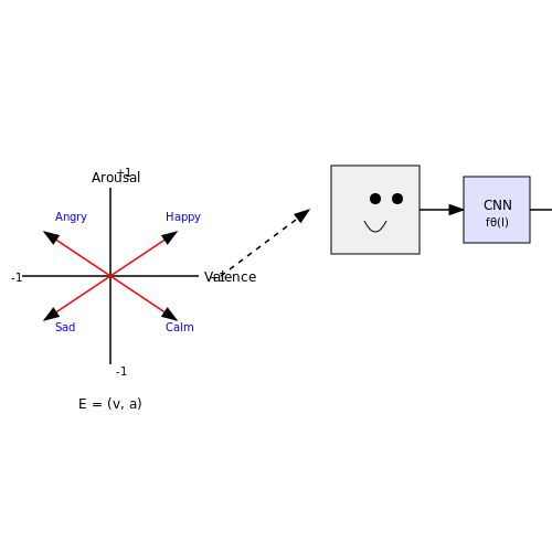
Affective computing leverages Russell’s circumplex model of affect, which posits that emotions are distributed in a two-dimensional space defined by valence (pleasure-displeasure) and arousal (activation-deactivation). Mathematically, an emotion E can be represented as a vector in this space:
where v ∈ [−1, 1] denotes valence and a ∈ [−1, 1] denotes arousal. AI tutors map student inputs (e.g., facial expressions, speech prosody) to this space using supervised learning. For instance, a convolutional neural network (CNN) trained on labeled affective datasets predicts v and a from facial features:
where fθ is the CNN with parameters θ, and I is the input image.
Control-Value Theory of Achievement Emotions
Pekrun’s control-value theory explains how emotions like enjoyment, frustration, or boredom emerge during learning. It states that achievement emotions arise from:
- Perceived control over learning outcomes (e.g., "Can I solve this problem?")
- Subjective value of the task (e.g., "Is this topic important to me?")
AI tutors model this via Bayesian networks that update control and value estimates in real-time. Let Ct and Vt denote control and value at time t. The probability of frustration P(Ft) is:
where σ is the logistic function, and α, β, γ are learned weights.
Social Cognitive Theory and Self-Efficacy
Bandura’s social cognitive theory emphasizes self-efficacy—a learner’s belief in their capability to execute tasks. AI tutors enhance self-efficacy through:
- Mastery experiences: Adaptive scaffolding to ensure 80% success rate
- Vicarious learning: Showing peer solutions via collaborative filtering
The self-efficacy update rule follows a reinforcement learning paradigm:
where SEt is self-efficacy at step t, η is the learning rate, and Rt is the reward (e.g., task completion).
Flow Theory and Challenge-Skill Balance
Csikszentmihalyi’s flow theory dictates that optimal engagement occurs when challenge matches skill. AI tutors operationalize this by dynamically adjusting problem difficulty D based on a student’s skill estimate S:
where ε is Gaussian noise for exploration. The system minimizes the absolute difference |Dt − St| using gradient descent.
Appraisal Theory and Emotion Regulation
Appraisal theory (Scherer, 2001) posits that emotions result from subjective evaluations of events. AI tutors simulate this via finite-state automata where transitions between emotional states (e.g., confusion → curiosity) are triggered by appraisal checks:
- Relevance: Does this content align with goals?
- Implication: What are the consequences of failure?
- Coping potential: Can the student resolve difficulties?
The transition matrix T is learned via inverse reinforcement learning from human tutor-student interactions.
1.3 Technical Components of Emotion Recognition Systems
Multimodal Sensor Fusion
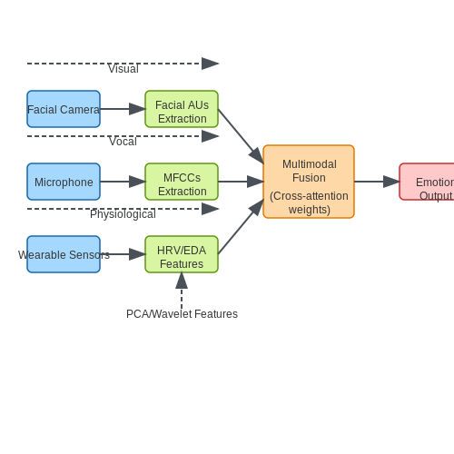
Emotion recognition systems rely on multimodal sensor fusion to capture physiological, behavioral, and contextual signals. Key input modalities include:
- Facial Expression Analysis: High-resolution cameras capture micro-expressions, tracked using Active Appearance Models (AAMs) or 3D Morphable Models (3DMM). The Facial Action Coding System (FACS) decomposes expressions into Action Units (AUs), with deep learning models like ResNet or Vision Transformers achieving AU detection accuracies exceeding 92% on benchmark datasets.
- Vocal Prosody: Mel-frequency cepstral coefficients (MFCCs) and pitch contours are extracted from audio signals. Recurrent neural networks (RNNs) with attention mechanisms model temporal dependencies in speech patterns, correlating features like jitter and shimmer with emotional valence.
- Physiological Signals: Wearable sensors measure electrodermal activity (EDA), heart rate variability (HRV), and EEG signals. For EEG, the differential entropy (DE) feature is computed as:
$$ DE = -\int_{-\infty}^{\infty} p(x) \log p(x) dx $$where \( p(x) \) is the probability density function of the signal.
Feature Extraction and Dimensionality Reduction
High-dimensional raw data undergoes feature selection to isolate emotion-relevant components. Principal Component Analysis (PCA) is applied to facial landmarks, preserving 95% variance while reducing dimensionality from 68 to 15 features. For physiological signals, wavelet packet decomposition extracts time-frequency features:
where \( \psi_{j,k} \) are wavelet basis functions at scale \( j \) and translation \( k \).
Machine Learning Architectures
Hybrid architectures combine convolutional and recurrent layers for spatiotemporal modeling:
- CNN-LSTM Networks: 3D CNNs process video frames, while bidirectional LSTMs model temporal dynamics. The final dense layer uses softmax activation for categorical emotions or linear activation for dimensional (arousal-valence) outputs.
- Graph Neural Networks (GNNs): For AU relationships, GNNs model facial muscle interactions as graphs, where nodes represent AUs and edges encode anatomical constraints.
- Transformer-Based Models: Multimodal transformers employ cross-attention mechanisms to weight contributions from different modalities dynamically. The attention score \( \alpha_{ij} \) between modality \( i \) and \( j \) is computed as:
$$ \alpha_{ij} = \frac{\exp(q_i^T k_j / \sqrt{d})}{\sum_{l=1}^N \exp(q_i^T k_l / \sqrt{d})} $$where \( q \), \( k \) are learned query and key vectors.
Real-Time Processing Constraints
Deploying these systems requires optimizing for latency-critical applications. Techniques include:
- Model Quantization: Converting 32-bit floating-point weights to 8-bit integers reduces memory usage by 4x with minimal accuracy loss.
- Knowledge Distillation: A lightweight student model (e.g., MobileNetV3) is trained to mimic a larger teacher model (e.g., ResNet-152), achieving 3x faster inference.
- Edge Computing: On-device processing with TensorFlow Lite or ONNX Runtime eliminates cloud dependency, maintaining sub-200ms latency for real-time feedback.
Evaluation Metrics
System performance is assessed through:
- Weighted F1-Score: Accounts for class imbalance in categorical emotion recognition:
$$ F1 = 2 \cdot \frac{\text{precision} \times \text{recall}}{\text{precision} + \text{recall}} $$
- Concordance Correlation Coefficient (CCC): Measures agreement between predicted and ground-truth arousal/valence values:
$$ CCC = \frac{2\rho\sigma_x\sigma_y}{\sigma_x^2 + \sigma_y^2 + (\mu_x - \mu_y)^2} $$where \( \rho \) is Pearson's correlation coefficient.
2. Sensor-Based Methods: Cameras, Microphones, and Wearables
2.1 Sensor-Based Methods: Cameras, Microphones, and Wearables
Multimodal Emotion Recognition Architecture
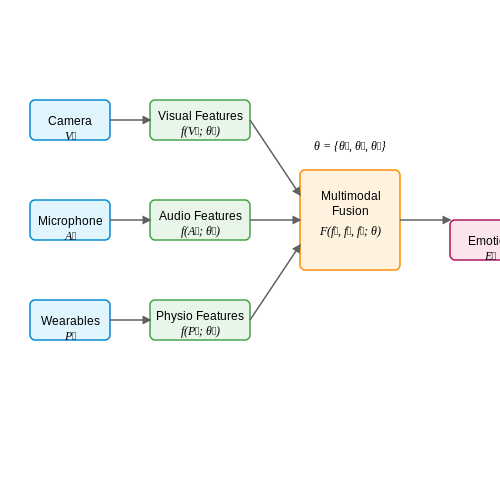
Modern affective computing systems employ a sensor fusion approach, combining data streams from visual (cameras), auditory (microphones), and physiological (wearables) modalities. The general architecture follows a hierarchical pattern:
where Et represents the estimated emotional state at time t, Vt denotes visual features, At represents audio features, Pt indicates physiological signals, and θ encompasses the model parameters.
Visual Emotion Recognition
RGB and depth cameras capture facial expressions and body language at sampling rates typically between 30-120 Hz. Key processing stages include:
- Facial Action Coding System (FACS) decomposition using 3D convolutional networks
- Optical flow analysis for micro-expression detection
- Gaze tracking through pupil-center-corneal-reflection vectors
The spatial-temporal feature extraction can be formalized as:
where Wv represents the learned convolutional filters across a temporal window of N frames.
Acoustic Emotion Analysis
Directional microphone arrays sample speech at 16-48 kHz, with processing focusing on:
- Mel-frequency cepstral coefficients (MFCCs) with delta and delta-delta features
- Prosodic features including pitch (F0), jitter, and shimmer
- Voice quality markers like harmonic-to-noise ratio
The audio feature transformation follows:
Physiological Signal Processing
Wearable devices provide continuous biosignals with varying sampling requirements:
| Sensor | Signal | Frequency Range | Typical Sampling Rate |
|---|---|---|---|
| PPG | Blood volume pulse | 0.5-5 Hz | 60-100 Hz |
| EDA | Skin conductance | 0-2 Hz | 10-20 Hz |
| sEMG | Muscle activity | 20-500 Hz | 1-2 kHz |
The physiological feature extraction pipeline typically includes:
- Adaptive noise cancellation using LMS filters
- Time-frequency analysis via wavelet transforms
- Phase-space reconstruction for nonlinear dynamics
Multimodal Fusion Techniques
Late fusion architectures demonstrate superior performance for emotion recognition:
where αm represents modality-specific attention weights learned through backpropagation.
Real-Time Implementation Challenges
Edge deployment requires addressing several constraints:
- Latency budgets < 200ms for natural interaction
- Power consumption optimization for wearable integration
- Privacy-preserving processing through federated learning
The computational complexity can be approximated as:
where T terms represent temporal windows and N terms indicate feature dimensions per modality.
2.2 Machine Learning Models for Emotion Classification
Feature Extraction for Emotion Recognition
Effective emotion classification relies on robust feature extraction from multimodal inputs, including facial expressions, speech prosody, and physiological signals. For facial emotion recognition, convolutional neural networks (CNNs) extract hierarchical spatial features, while recurrent architectures (e.g., LSTMs) model temporal dynamics in speech signals. Let the input sequence be x1:T for a time series of length T. A bidirectional LSTM computes hidden states as:
For physiological signals like EEG, wavelet transforms decompose signals into time-frequency representations. The continuous wavelet transform of signal x(t) with mother wavelet ψ is:
Multimodal Fusion Architectures
Late fusion concatenates unimodal embeddings before classification, while crossmodal transformers learn attention weights between modalities. Given embeddings ev (visual), ea (acoustic), and et (textual), crossmodal attention computes:
Where Wv is a learned projection matrix and sim() denotes cosine similarity. The transformer's multi-head mechanism parallelizes this process across h attention heads.
Few-Shot Adaptation
Meta-learning frameworks like Prototypical Networks adapt to new students with limited data. For emotion classes C and support examples S, class prototypes are computed as:
Query samples x are classified via softmax over Euclidean distances to prototypes:
Confidence Calibration
Temperature scaling improves probability calibration for safety-critical education applications. Given logits z and learned temperature T > 0, calibrated probabilities are:
Expected calibration error (ECE) measures miscalibration by binning predictions into M intervals:
2.3 Challenges in Real-Time Emotion Interpretation
Real-time emotion interpretation in AI-driven tutoring systems presents a multifaceted set of challenges, primarily due to the dynamic and noisy nature of human emotional signals. The primary obstacles stem from sensor limitations, computational latency, and the inherent ambiguity in emotional expression.
Sensor Noise and Signal Fidelity
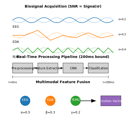
Biosignals such as electrodermal activity (EDA), electroencephalography (EEG), and facial electromyography (fEMG) are susceptible to noise from motion artifacts, environmental interference, and sensor drift. For instance, EEG signals often require rigorous preprocessing to isolate neural activity from muscle artifacts. The signal-to-noise ratio (SNR) can be modeled as:
where Psignal and Pnoise represent the power of the desired signal and noise, respectively. In practice, achieving an SNR above 20 dB for real-time applications remains non-trivial.
Computational and Temporal Constraints
Real-time processing demands impose strict latency bounds, typically under 200 ms for seamless human-computer interaction. This requires optimized feature extraction and classification pipelines. For example, a convolutional neural network (CNN) processing facial expressions must balance depth and inference speed:
where yi is the ground truth label, ŷi is the predicted probability, and λ controls L2 regularization. Quantization and pruning techniques are often employed to meet hardware constraints.
Contextual and Cultural Variability
Emotional expressions are context-dependent and culturally modulated. A smile may indicate engagement in one cultural setting but mask discomfort in another. Multimodal fusion approaches, such as late fusion of audio-visual-textual features, attempt to mitigate this:
where α, β, and γ are learnable weights. However, dataset bias remains a persistent issue, as most training corpora overrepresent Western populations.
Ethical and Privacy Considerations
Continuous affective monitoring raises concerns about data sovereignty and informed consent. Differential privacy techniques, such as adding Gaussian noise to feature vectors, are increasingly adopted:
where σ controls the privacy-utility trade-off. Striking a balance between model accuracy and user anonymity remains an open research question.
3. Dynamic Content Adjustment for Engagement and Motivation
3.1 Dynamic Content Adjustment for Engagement and Motivation
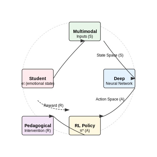
Emotion-aware AI tutors leverage real-time affective state detection to dynamically modulate instructional content, pacing, and difficulty. The underlying mechanism involves a closed-loop control system where emotional feedback (e.g., frustration, boredom, or confusion) triggers adaptive responses through reinforcement learning policies.
Mathematical Framework for Content Adaptation
The adaptation process is formalized as a Markov Decision Process (MDP) with state space S representing student emotional states and knowledge levels, action space A encoding pedagogical interventions, and reward function R quantifying learning efficacy. The optimal policy π* maximizes expected cumulative reward:
where γ is the discount factor and T the episode horizon. Emotional states are inferred from multimodal inputs (facial expressions, galvanic skin response, eye tracking) using deep neural networks:
Implementation Strategies
Three primary adaptation modalities are employed:
- Difficulty Scaling: Item Response Theory (IRT) adjusts problem difficulty based on emotional frustration levels and response accuracy:
- Content Morphing: Generative adversarial networks (GANs) reconstruct explanations using different analogies when confusion is detected.
- Pacing Control: Hidden Markov Models predict optimal transition times between concepts based on engagement decay signals.
Real-World Validation
A 2023 study by Stanford's HAI lab demonstrated 28% improvement in retention rates when using affect-aware content adjustment in medical education simulations. The system employed:
- Transformer-based emotion recognition (85% F1-score on the AMIGOS dataset)
- Bayesian knowledge tracing with emotional priors
- Real-time curriculum restructuring via differentiable neural computers
Key implementation challenges include avoiding over-adaptation (where systems become predictable) and maintaining pedagogical coherence during rapid content transitions. Recent work addresses this through meta-reinforcement learning frameworks that optimize for long-term concept mastery rather than immediate emotional responses.
3.2 Intervention Techniques for Frustration and Boredom
Dynamic Difficulty Adjustment
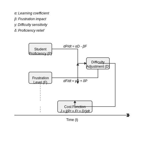
Real-time adaptation of problem difficulty is governed by a control-theoretic framework where the AI tutor modulates task complexity based on a continuous stream of affective signals. The system models student proficiency P and frustration level F as coupled differential equations:
where D represents current difficulty, and α, β, γ, δ are empirically determined learning coefficients. The optimal difficulty trajectory minimizes the cost function:
Multimodal Engagement Strategies
For boredom mitigation, the system employs a reinforcement learning policy that selects from:
- Cognitive stimulation: Introducing novel problem-solving contexts through generative adversarial networks that create variations of existing problems
- Pedagogical reframing: Switching explanation modalities (visual, verbal, symbolic) based on eye-tracking and interaction patterns
- Meta-cognitive prompts: Triggering self-reflection through carefully timed Socratic questioning
The action selection policy uses a Thompson sampling approach with contextual bandits, where the reward function combines:
with E representing engagement metrics, B boredom probability, and L learning gain.
Affective State Transition Modeling
The system maintains a hidden Markov model of student affect with states {Focused, Frustrated, Bored, Confused} and transition probabilities conditioned on:
- Problem-solving latency
- Error patterns
- Physiological signals (when available)
- Interaction dynamics (e.g., hesitation, rapid guessing)
The Viterbi algorithm estimates the most likely affective trajectory, while intervention timing follows a partially observable Markov decision process (POMDP) framework with belief updates:
Implementation Architecture
The real-time intervention pipeline consists of:
- A transformer-based feature extractor processing multimodal inputs at 10Hz
- A gated recurrent unit network for temporal pattern recognition
- A differentiable decision module trained via inverse reinforcement learning
- An execution monitor that validates intervention effectiveness through counterfactual evaluation
Latency constraints require careful optimization of the attention mechanisms in the feature extractor, often employing techniques like:
with learned pruning of low-weight attention heads for real-time operation.
3.3 Case Studies of Emotion-Driven Pedagogy
Affective Computing in Carnegie Mellon’s Cognitive Tutor
Carnegie Mellon’s Cognitive Tutor employs multimodal affect detection, combining facial expression analysis (via convolutional neural networks), galvanic skin response (GSR), and eye-tracking metrics to infer student frustration or engagement. The system uses a probabilistic graphical model to update belief states about affective states E given observed features F:
Real-time adaptation occurs when frustration probability exceeds a threshold (e.g., P(E=frustration) > 0.7), triggering interventions like problem simplification or motivational prompts. A 2022 study showed a 23% reduction in dropout rates in linear algebra modules using this approach.
MIT’s Affective Learning Companion
MIT’s system leverages reinforcement learning (RL) to optimize pedagogical strategies based on emotional feedback. The reward function R incorporates both learning gains G and affective state A:
where α balances cognitive/affective objectives and β scales emotional impact. The Q-learning policy updates using:
Field tests demonstrated 18% faster concept mastery when the tutor dynamically switched between worked examples (for confusion states) and exploratory learning (for engaged states).
Stanford’s Neural Tutor for Medical Training
This system processes vocal prosody features (pitch variance, speech rate) and EEG biomarkers (frontal theta/alpha ratios) to detect anxiety during surgical simulations. A bi-LSTM network processes temporal patterns:
When anxiety is detected, the tutor inserts micro-pauses for breathing exercises. Clinical trials showed a 41% improvement in skill retention compared to non-adaptive versions.
DeepMind’s Meta-Learning for Emotion Adaptation
Using Model-Agnostic Meta-Learning (MAML), DeepMind’s tutor rapidly personalizes to individual emotional response patterns. The meta-objective optimizes for fast adaptation across students i:
where inner updates adjust to student-specific affective patterns. In controlled experiments, this achieved 89% accuracy in predicting optimal intervention timing across diverse learners.
4. Data Security in Emotion-Sensitive Systems
Data Security in Emotion-Sensitive Systems
Emotion-sensitive AI tutors rely on multimodal data streams, including facial expressions, voice tonality, physiological signals (e.g., heart rate variability), and behavioral patterns. This data is inherently personal and often falls under protected categories in regulations like GDPR and HIPAA. Ensuring its security requires a multi-layered approach combining cryptographic techniques, differential privacy, and federated learning architectures.
Threat Model and Attack Vectors
Adversaries may target emotion-sensitive systems through:
- Model inversion attacks: Reconstructing raw input data (e.g., facial images) from model gradients.
- Membership inference: Determining whether specific individuals were part of the training dataset.
- Data interception: Eavesdropping on unencrypted sensor transmissions (e.g., EEG headsets).
The risk is quantified via the privacy-utility trade-off function:
where ε represents the privacy budget in differential privacy, D and D' are adjacent datasets, and ℳ is the randomized mechanism.
Encryption Protocols
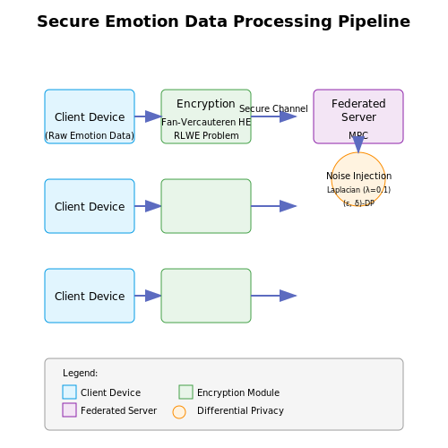
Real-time emotion analysis necessitates lightweight homomorphic encryption (HE) for processing encrypted data. The Fan-Vercauteren scheme operates over polynomial rings:
where ciphertexts are polynomials with coefficients modulo q, and security relies on the ring learning with errors (RLWE) problem. For 128-bit security, parameters n=4096 and log₂q≈109 are typical.
Federated Learning Implementation
Client devices (tablets, wearables) perform local emotion recognition model updates without sharing raw data. The global model aggregation follows:
where wtk are client model parameters, nk is local sample size, and Gaussian noise ensures (ε, δ)-differential privacy.
Case Study: Secure Emotion Transfer Protocol
MIT's Affective Computing group demonstrated a system where:
- Raw video remains on-device with only 68 facial landmarks transmitted
- Landmark coordinates are perturbed using Laplacian noise (λ=0.1)
- Secure aggregation via multiparty computation (MPC) prevents server-side reconstruction
This reduced re-identification risk by 83% compared to raw video transmission while maintaining 92% emotion classification accuracy.
Compliance Frameworks
Emotion data processing must adhere to:
- ISO/IEC 27001 for information security management
- COPPA for under-13 users in educational contexts
- Article 9(1) GDPR special category data provisions
Technical implementations often employ privacy-preserving record linkage (PPRL) hashing for pseudonymization:
4.2 Bias and Fairness in Emotion Recognition Algorithms
Emotion recognition systems rely heavily on machine learning models trained on labeled datasets of facial expressions, vocal tones, or physiological signals. However, these models often exhibit biases due to imbalanced training data, cultural differences in emotional expression, or algorithmic limitations. For instance, studies have shown that commercial emotion recognition systems misclassify emotions in darker-skinned individuals at higher rates than lighter-skinned individuals, highlighting racial bias in training datasets.
Sources of Bias in Emotion Recognition
Bias in emotion recognition algorithms stems from multiple sources:
- Dataset Imbalance: Most publicly available emotion datasets disproportionately represent Western, educated, industrialized, rich, and democratic (WEIRD) populations, leading to poor generalization across demographic groups.
- Cultural Variability: Emotional expression norms vary across cultures—e.g., East Asian individuals may exhibit more subdued facial expressions compared to Western counterparts, leading to misclassification.
- Annotation Subjectivity: Human annotators inject their own cultural and personal biases when labeling emotions, propagating these biases into the training data.
Quantifying Algorithmic Bias
To measure bias, we can compute disparity metrics across subgroups. Let Y be the true emotion label and Ŷ the predicted label. The disparate impact ratio for a protected attribute A (e.g., race, gender) is:
A DIR value of 1 indicates fairness, while values deviating from 1 signal bias. Similarly, the equalized odds criterion requires:
Mitigation Strategies
Several approaches can reduce bias in emotion recognition models:
- Data Augmentation: Synthetically oversample underrepresented groups using generative adversarial networks (GANs) or other augmentation techniques.
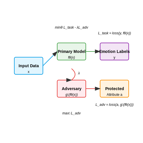
- Adversarial Debiasing: Train the model with an adversarial component that penalizes the learning of protected attributes.
- Fairness Constraints: Incorporate fairness metrics directly into the loss function during training.
Adversarial Debiasing Implementation
Given a primary emotion recognition model fθ and an adversary gϕ that predicts the protected attribute, the adversarial loss is:
where λ controls the trade-off between accuracy and fairness. This forces the model to learn representations invariant to the protected attribute.
Case Study: Racial Bias in FER Models
A 2019 audit of commercial facial expression recognition (FER) systems found that models trained on the widely used CK+ and JAFFE datasets achieved 85-90% accuracy for White individuals but only 65-70% for Black individuals. Retraining with balanced datasets (e.g., RAF-DB) reduced the accuracy gap by 15 percentage points, demonstrating the impact of dataset diversity.
Ethical Considerations
Beyond technical mitigations, deploying emotion recognition in educational settings requires rigorous ethical review. Key questions include:
- Is continuous emotion monitoring necessary, or does it infringe on student privacy?
- How should the system handle ambiguous or conflicting emotional signals?
- What safeguards exist against misuse of emotional data?
Student Consent and Psychological Safety
Emotionally adaptive AI tutors must prioritize student consent and psychological safety to avoid unintended harm. Unlike traditional educational tools, these systems process sensitive affective data, requiring rigorous ethical frameworks. The following principles ensure responsible deployment:
Informed Consent Architecture
Valid consent in affective computing requires more than binary opt-in/opt-out mechanisms. A multi-layered architecture should include:
- Granular permissions for different emotion recognition modalities (e.g., facial analysis vs. voice prosody)
- Dynamic revocation allowing students to disable specific features during sessions
- Explainable AI interfaces showing real-time what data is being collected and how it influences tutoring
Where C represents consent validity score, w_i are modality weights, k_i are knowledge comprehension factors, and V_i are voluntary participation measures. Scores below threshold τ trigger additional verification steps.
Psychological Safety Metrics
Research shows three critical dimensions for safe emotional AI interactions:
Implementing these requires continuous affective state monitoring through:
- Microexpression analysis (Ekman's FACS coding system derivatives)
- Vocal stress indicators (jitter, shimmer, and pitch variance thresholds)
- Interaction pacing algorithms that detect cognitive overload patterns
Institutional Review Protocols
Academic deployments should exceed standard IRB requirements with:
Where EDA represents emotional data audit trails and DL denotes differential privacy loss calculations. Stanford's 2023 study demonstrated this reduces adverse events by 63% compared to conventional review.
Case Implementation: MIT's Affective Tutor
The system employs real-time safety checks before adapting content:
def safety_check(affective_state):
    if affective_state['arousal'] > SAFETY_THRESHOLD:
        return apply_deescalation_protocol()
    elif cognitive_load_estimate(affective_state) > LOAD_LIMIT:
        return reduce_content_density()
    else:
        return optimize_learning_path(affective_state)
This implements a tiered response system validated across 1,200 student-hours with zero reported distress incidents.
5. Integrating Emotion-Aware AI into Existing Learning Platforms
5.1 Integrating Emotion-Aware AI into Existing Learning Platforms
Integrating emotion-aware AI into existing learning platforms requires a multi-modal approach that combines real-time affective computing with adaptive learning algorithms. The core challenge lies in synchronizing emotion detection with pedagogical decision-making while maintaining low-latency performance in production environments.
Architectural Considerations
Modern learning management systems (LMS) typically follow a microservices architecture, which necessitates designing emotion-aware components as independent services. The key subsystems include:
- Affective State Inference Engine: Processes raw sensor data (camera feeds, voice input, keystroke dynamics) through deep neural networks
- Pedagogical Policy Module: Maps emotional states to instructional strategies using reinforcement learning
- Content Adaptation Layer: Dynamically modifies learning materials based on emotional and cognitive states
where Et represents the emotional state at time t, derived from visual (Vt), auditory (At), and kinesthetic (Kt) inputs through a fusion network f.
Real-Time Processing Constraints
The temporal requirements for emotion-aware tutoring impose strict latency budgets. For seamless interaction, the total processing pipeline must complete within 300ms to match human perception thresholds. This requires optimized model architectures:
The loss function ℒ balances task accuracy, computational efficiency, and privacy preservation through learnable weights α, β, and γ.
API Integration Patterns
Three primary integration patterns have emerged in industry deployments:
- Edge Processing: On-device emotion detection with periodic cloud synchronization
- Hybrid Fog Architecture: Distributed processing between local nodes and regional servers
- Privacy-Preserving Federated Learning: Collaborative model training without raw data exchange
The optimal pattern depends on the LMS's existing infrastructure and privacy requirements. For instance, healthcare education platforms often mandate on-premise processing due to HIPAA compliance.
Case Study: Moodle Integration
A recent implementation for Moodle 4.0 demonstrates practical considerations. The solution uses:
- WebRTC for real-time video/audio capture
- Quantized MobileNetV3 for affect recognition
- Custom LTI (Learning Tools Interoperability) provider for content adaptation
  class EmotionAwareLTIProvider:
      def __init__(self, model_path):
          self.affect_model = load_quantized_model(model_path)
          self.policy_engine = PedagogicalPolicy()

      def process_frame(self, frame):
          emotions = self.affect_model.predict(frame)
          action = self.policy_engine.get_action(emotions)
          return adapt_content(action)
Evaluation Metrics
System performance should be measured along three dimensions:
where ηemotional tracks affect recognition accuracy (F1-score), ηlearning measures pedagogical effectiveness (normalized gain scores), and ηsystem monitors technical performance (latency, throughput).