Feedback-Driven Prompt Iteration Systems
1. Core Principles of Prompt Engineering
Core Principles of Prompt Engineering
Prompt engineering is the systematic design and optimization of input queries to guide large language models (LLMs) toward desired outputs. At its core, it involves understanding the model's internal representations, tokenization mechanics, and response generation dynamics. Advanced practitioners leverage techniques such as chain-of-thought prompting, few-shot learning, and controlled generation constraints to achieve precise, reproducible results.
Tokenization and Context Windows
LLMs process text as sequences of tokens, where subword tokenization (e.g., Byte Pair Encoding) splits inputs into discrete units. The model's context window, typically 2048 to 128k tokens, imposes hard limits on input length. Token efficiency becomes critical when iterating prompts, as redundant phrasing consumes valuable context space. For a prompt P with n tokens, the remaining context for the response R is constrained by:
where k accounts for system tokens and overhead. Exceeding Ctotal triggers truncation or rejection.
Semantic Density and Precision
High-performance prompts maximize semantic density—the information-to-token ratio—while minimizing ambiguity. This requires:
- Lexical specificity: Using domain-specific terminology (e.g., "transformer attention weights" vs. "AI components")
- Structural constraints: Explicit output formatting (JSON, YAML) or step-by-step reasoning directives
- Negative examples: Defining undesired outputs through contrastive statements
For example, a physics-focused prompt might specify:
"Derive the time dilation equation from Lorentz transformations. Show all steps symbolically before substituting numerical values."
Feedback-Driven Optimization
Effective prompt iteration relies on measurable evaluation metrics. For classification tasks, precision and recall can guide refinements:
In generative tasks, semantic similarity scores (e.g., BERTScore) between outputs and gold-standard references provide quantitative feedback. Automated testing frameworks execute prompt variants against validation sets, identifying failure modes through confusion matrices or embedding space clustering.
Temperature and Sampling Dynamics
The temperature parameter T controls output stochasticity in autoregressive models. Lower values (0.1-0.5) produce deterministic, peak-probability responses, while higher values (0.7-1.2) encourage creativity at the risk of incoherence. For technical domains, optimal sampling often combines low temperature with top-k or nucleus sampling (top-p):
where V is the vocabulary space. This balances precision with controlled exploration of the solution space.
Role of Feedback in Iterative Prompt Refinement
Feedback mechanisms serve as the optimization engine in prompt refinement cycles, transforming subjective human evaluations into quantifiable gradients for prompt improvement. Unlike traditional supervised learning where loss functions provide direct error signals, prompt optimization relies on implicit feedback loops that balance semantic coherence with task-specific performance metrics.
Mathematical Formulation of Feedback-Driven Optimization
The prompt refinement process can be modeled as a Markov decision process where each iteration t generates a new prompt variant pt based on feedback from the previous iteration. The quality function Q(pt) maps prompt features to performance scores:
where α, β, γ are tunable weights reflecting domain priorities. The gradient for prompt update derives from partial derivatives of Q with respect to prompt components:
Feedback Taxonomy in Prompt Engineering
Advanced refinement systems utilize multi-modal feedback channels:
- Explicit human ratings: Direct scoring of output quality on Likert scales
- Implicit behavioral signals: User edit distance from model outputs
- Model confidence metrics: Log probability distributions over generated tokens
- Adversarial discriminators: Secondary models evaluating output coherence
Case Study: Reinforcement Learning from Human Feedback (RLHF)
Modern LLMs employ preference modeling where human feedback trains a reward model Rφ that predicts scalar rewards for prompt-output pairs. The policy gradient update becomes:
where πθ represents the LLM's policy. Practical implementations use proximal policy optimization (PPO) to constrain updates within trust regions.
Feedback Latency Considerations
Real-world systems must balance feedback quality with iteration speed. The optimal sampling period Δt between refinements follows:
where λ controls the exploration-exploitation tradeoff. Systems handling safety-critical applications typically implement shorter feedback cycles with human-in-the-loop verification.
Error Propagation in Iterative Refinement
Feedback noise introduces compounding errors across iterations. For a system with feedback variance σ2, the n-th iteration error grows as:
where γ is the contraction factor of the refinement operator. This necessitates robust filtering of outlier feedback points through statistical validation gates.

Key Metrics for Evaluating Prompt Effectiveness
Quantitative Metrics
To rigorously assess prompt performance, several quantitative metrics are essential. Task accuracy measures the correctness of the model's output relative to a ground truth, computed as:
Precision and recall are critical for classification tasks, where:
For generative tasks, BLEU score and ROUGE-L evaluate text similarity to reference outputs. BLEU computes n-gram overlap, while ROUGE-L measures the longest common subsequence.
Latency and Computational Efficiency
Prompt response time directly impacts user experience. Inference latency is measured from prompt submission to completion, while throughput quantifies requests processed per second. For resource-constrained deployments, FLOPs per token and memory footprint are key constraints.
Human Evaluation Metrics
Quantitative metrics alone are insufficient. Human-rated quality scores on scales (1-5) assess coherence, relevance, and fluency. Adversarial testing probes for robustness against edge cases, measuring failure modes under distribution shifts.
Adaptive Metrics for Iterative Refinement
Feedback loops require dynamic metrics. Delta accuracy tracks improvement between prompt versions:
User engagement signals (e.g., dwell time, follow-up queries) provide implicit feedback. Gradient-based sensitivity analysis identifies critical prompt components by computing:
where \( p_i \) represents the i-th prompt token and \( \mathcal{L} \) is the loss function.
Cross-Modal Consistency
For multimodal systems, cross-modal alignment scores measure semantic consistency between generated text and associated images/audio. This is computed using CLIP-like embeddings for vision-language tasks.
2. Types of Feedback: Explicit vs. Implicit
Types of Feedback: Explicit vs. Implicit
Feedback mechanisms in prompt iteration systems are broadly categorized into explicit and implicit feedback, each serving distinct roles in refining model outputs. Understanding their differences, advantages, and limitations is critical for designing robust feedback-driven systems.
Explicit Feedback
Explicit feedback consists of direct, user-provided evaluations of model outputs, such as ratings, rankings, or textual corrections. This feedback is intentionally solicited and structured, making it highly interpretable for model refinement. For instance, a user might rate a generated response on a Likert scale (e.g., 1–5) or provide a binary label (e.g., "relevant/irrelevant").
Mathematically, explicit feedback can be modeled as a supervised learning problem. Given a prompt x and model output y, the feedback f is a discrete or continuous signal:
Key properties of explicit feedback include:
- High signal-to-noise ratio: Directly reflects user intent.
- Sparse: Requires active user participation, leading to lower data volume.
- Bias risks: May suffer from subjectivity or anchoring effects.
Implicit Feedback
Implicit feedback is inferred from user behavior rather than explicitly provided. Examples include dwell time on generated content, click-through rates, or edit distance in user-modified outputs. This feedback is passive and unstructured, offering a richer but noisier signal.
Implicit feedback often follows an inverse reinforcement learning paradigm, where the goal is to infer a reward function R from observed behavior B:
Challenges with implicit feedback include:
- Noise: Behavior may not align with true preferences (e.g., accidental clicks).
- Ambiguity: Requires careful interpretation (e.g., long dwell time could indicate interest or confusion).
- Scalability: Easier to collect at volume compared to explicit feedback.
Practical Trade-offs
Hybrid systems often combine both feedback types. For example, explicit feedback can calibrate implicit signals via a weighting parameter α:
Case studies show that implicit feedback dominates in production systems (e.g., search engines) due to scalability, while explicit feedback is reserved for high-stakes scenarios (e.g., medical diagnostics) where precision is paramount.
Automated Feedback Systems: Metrics and Tools
Automated feedback systems in prompt engineering rely on quantifiable metrics to evaluate and iteratively improve prompts. These systems typically employ a combination of statistical, semantic, and task-specific evaluation criteria to assess prompt effectiveness.
Core Evaluation Metrics
The most critical metrics for automated feedback systems fall into three categories:
- Task Performance Metrics: Measure how well the generated output satisfies the intended task requirements
- Consistency Metrics: Evaluate the stability of outputs across multiple generations
- Semantic Metrics: Assess the linguistic and conceptual quality of outputs
Task Performance Metrics
For classification tasks, standard evaluation metrics include:
For generation tasks, metrics like BLEU, ROUGE, and METEOR score are commonly used. The BLEU score calculation for n-gram precision is:
where BP is the brevity penalty and pₙ is the modified n-gram precision.
Consistency Metrics
Output consistency is measured through:
where K is the number of generations and d(yᵢ, yⱼ) is a distance metric between outputs.
Automated Feedback Tools
Modern prompt engineering pipelines incorporate several types of automated feedback tools:
- Static Analysis Tools: Analyze prompt structure and syntax before execution
- Dynamic Evaluation Tools: Assess model outputs during runtime
- Meta-Evaluation Tools: Combine multiple metrics into composite scores
Dynamic Evaluation Architecture
A typical dynamic evaluation system implements the following components:
- Prompt execution engine
- Output capture module
- Metric computation layer
- Feedback aggregation system
The feedback aggregation often uses weighted scoring:
where wᵢ are learned weights and mᵢ are normalized metric scores.
Implementation Considerations
When implementing automated feedback systems, key considerations include:
- Metric selection based on task requirements
- Computational efficiency of evaluation
- Feedback latency constraints
- Correlation between automated metrics and human judgment
Recent research shows that combining 3-5 complementary metrics typically provides the most robust feedback, with the optimal combination varying by application domain.

Human-in-the-Loop Feedback Strategies
Active Learning for Prompt Refinement
Active learning frameworks integrate human feedback to iteratively improve prompt quality. The system selects prompts where model uncertainty is highest, presenting them to human annotators for refinement. The uncertainty measure U(p) for a prompt p can be quantified using entropy over model predictions:
where Y is the set of possible outputs and P(y|p) is the model's predicted probability distribution. Human feedback is then incorporated through Bayesian updating:
The mixing parameter α controls the relative weight of human vs. model judgments, typically set empirically through cross-validation.
Preference-Based Reward Modeling
Human feedback can be captured through pairwise comparisons between model outputs. For prompt p generating outputs o₁ and o₂, the Bradley-Terry model estimates the probability that humans prefer o₁ over o₂:
where R(o,p) is a learned reward function. The reward model is trained using maximum likelihood estimation on human preference data, with regularization to prevent overfitting to sparse annotations.
Error-Driven Feedback Loops
Systems can detect potential errors by monitoring:
- Contradictions between model outputs for semantically similar prompts
- Low-confidence predictions (softmax probability < 0.3)
- Violations of predefined constraints (e.g., factual inaccuracies)
When errors are detected, the system triggers human review. The feedback is incorporated through gradient-based prompt tuning:
where L is the original loss and Lhuman is the loss derived from human corrections.
Multi-Armed Bandit Optimization
For real-time prompt improvement, Thompson sampling balances exploration of new prompt variants with exploitation of known high-performing prompts. Each prompt variant pi is modeled as a Bernoulli distribution with success probability θi:
Parameters α and β are updated based on human feedback:
- α ← α + 1 for positive feedback
- β ← β + 1 for negative feedback
The system samples from these distributions to select prompts that maximize expected reward while maintaining exploration of potentially better alternatives.
Feedback Aggregation Techniques
When multiple human annotators provide feedback, their inputs must be aggregated while accounting for individual biases. The Dawid-Skene model estimates true labels z and annotator confusion matrices π(j) through expectation-maximization:
where y(j) is the annotation from annotator j. This approach weights feedback from more reliable annotators more heavily in the final prompt refinement.

3. Data Collection and Preprocessing for Feedback Analysis
Data Collection and Preprocessing for Feedback Analysis
Feedback Data Sources
Effective feedback-driven prompt iteration systems rely on diverse data sources to capture user interactions comprehensively. Primary sources include:
- Explicit feedback: Direct user ratings, binary (thumbs up/down), or Likert-scale responses to generated outputs.
- Implicit feedback: Behavioral signals like dwell time, edit distance between user input and model output, or API call patterns.
- Conversational trajectories: Multi-turn dialogue sequences where later turns implicitly critique earlier responses.
- Human-in-the-loop annotations: Expert-labeled data for quality, safety, or alignment metrics.
In production systems, feedback signals often follow a power-law distribution where most users provide minimal explicit feedback. This necessitates careful handling of sparse, noisy signals through statistical imputation and confidence weighting.
Temporal Alignment of Feedback Signals
Feedback latency poses unique challenges - users may provide delayed ratings or revise initial impressions. For a prompt p generating response r at time t₀, we model feedback arrival as a stochastic process:
where λ₀ is the initial feedback intensity and β controls decay rate. The cumulative feedback weight for a prompt-response pair becomes:
where s(t) represents the feedback score at time t. This formulation downweights stale feedback while preserving recent signals.
Feature Engineering for Feedback Analysis
Raw feedback requires transformation into model-usable features. Key preprocessing steps include:
- Prompt-response embedding: Using contrastive learning to map (p,r) pairs into a joint embedding space where similar quality pairs cluster.
- Feedback disentanglement: Separating stylistic preferences (e.g., verbosity) from substantive quality metrics using factor analysis.
- Bias correction: Applying propensity weighting to address systematic under-reporting from certain user segments.
For textual feedback, transformer-based encoders with attention mechanisms extract nuanced signals. Given feedback text f, we compute:
where W_q and W_k are learned projections aligning feedback to prompt embeddings h_p.
Handling Noisy and Adversarial Feedback
Malicious or low-quality feedback requires robust filtering. A three-stage pipeline proves effective:
- Statistical filtering: Remove outliers beyond 3 median absolute deviations from user-specific baselines.
- Graph-based detection: Construct a bipartite graph of users and prompts, identifying suspicious clusters via random walk divergence.
- Generative verification: Use a secondary model to predict expected feedback distribution, flagging improbable ratings.
The final preprocessed dataset D' from raw data D undergoes:
where g(·) normalizes feedback scores and w_i represents confidence weights.

3.2 Algorithmic Approaches to Prompt Refinement
Feedback-driven prompt iteration relies on algorithmic methods to systematically refine prompts based on performance metrics. These approaches can be broadly categorized into gradient-based optimization, reinforcement learning, and evolutionary strategies, each with distinct mathematical formulations and practical trade-offs.
Gradient-Based Prompt Optimization
Modern language models with differentiable prompt embeddings enable gradient-based optimization. Given a prompt p and a loss function L(p) measuring task performance, we compute:
The prompt is then updated iteratively using:
where η is the learning rate. This approach works particularly well for soft prompts where the embedding space is continuous.
Reinforcement Learning for Discrete Prompt Refinement
For hard (discrete) prompts, policy gradient methods are more appropriate. The REINFORCE algorithm maximizes the expected reward R:
where θ represents the parameters of a prompt generation policy. Practical implementations often use advantage estimation and baseline subtraction to reduce variance.
Evolutionary Strategies
Evolutionary algorithms operate by maintaining a population of prompt variants. The fitness of each prompt pi is evaluated, and new generations are created through:
- Mutation: Random perturbations to prompt tokens or embeddings
- Crossover: Combining segments from high-performing prompts
- Selection: Keeping only the top-performing variants
The evolutionary process can be formalized as:
where Pt represents the population at generation t.
Hybrid Approaches
State-of-the-art systems often combine these methods. For example:
- Using gradient information to guide evolutionary mutations
- Applying RL to optimize the mutation parameters in an evolutionary algorithm
- Using gradient descent for continuous prompt components while applying RL for discrete parts
The choice of algorithm depends on the prompt representation (discrete vs. continuous), available feedback signals (exact gradients vs. reward signals), and computational constraints.

Case Studies: Successful Prompt Iteration Workflows
Large Language Model Optimization at OpenAI
OpenAI's iterative prompt refinement for GPT-4 demonstrates how systematic feedback loops can enhance model performance. Their workflow involves:
- Human-in-the-loop evaluation: Annotators score outputs across dimensions like accuracy, coherence, and safety.
- Quantitative metrics: Tracking precision (P), recall (R), and F1 scores across prompt variants.
- A/B testing: Comparing prompt versions on held-out validation sets.
Where P₀, R₀ represent baseline prompt performance and P₁, R₁ reflect the refined version. OpenAI achieved 18-22% F1 improvements through 5-7 iteration cycles.
Google's PaLM Instruction Tuning
Google Research optimized PaLM's prompts through:
- Automated feedback: Using smaller proxy models to predict human ratings.
- Gradient-based prompt search: Treating prompt tokens as continuous embeddings.
- Multi-objective optimization: Balancing accuracy, verbosity, and safety.
The gradient update rule for prompt embeddings θ:
Where η is the learning rate and ℒ combines cross-entropy and regularization terms. This approach reduced human evaluation rounds by 40% while maintaining quality.
Anthropic's Constitutional AI
Anthropic developed a novel feedback system for aligning Claude's outputs:
- Principle-based scoring: Evaluating responses against 50+ constitutional principles.
- Contrastive evaluation: Comparing outputs from competing prompts side-by-side.
- Adversarial probing: Stress-testing prompts with edge cases.
Their scoring function S for prompt p:
Where wᵢ are principle weights and λ controls risk aversion. This reduced harmful outputs by 63% across 12 safety categories.
Microsoft's Azure AI Prompt Engineering
Microsoft's production system combines:
- Real-time user feedback: Capturing thumbs up/down signals at scale.
- Automatic prompt versioning: Tracking performance drift over time.
- Ensemble prompting: Dynamically selecting optimal prompts per query type.
The ensemble selector uses a gating network G:
Where enc(q) encodes the query and W_g learns prompt combination weights. This increased customer satisfaction scores by 29%.
Meta's Crowdsourced Prompt Refinement
Meta's unique approach leverages:
- Distributed human computation: Thousands of contributors suggesting prompt variants.
- Evolutionary algorithms: Mutating and recombining successful prompts.
- Diversity sampling: Ensuring coverage across demographic groups.
Their fitness function for evolutionary selection:
This generated 14,000+ high-quality prompts covering 200+ languages and dialects.
4. Scalability and Computational Costs
4.2 Scalability and Computational Costs
Feedback-driven prompt iteration systems face significant computational challenges as they scale, particularly when deployed in production environments with high query volumes. The primary bottlenecks arise from three sources: the cost of inference, the overhead of feedback collection, and the iterative optimization process itself.
Inference Cost Scaling
Large language models (LLMs) exhibit near-linear increases in computational requirements with respect to sequence length and batch size. For a model with N parameters processing B batches of prompts with average length L, the floating-point operations (FLOPs) per forward pass scale as:
where dff represents feed-forward layer dimensions and dattn accounts for attention mechanisms. This quadratic dependence on sequence length becomes prohibitive when processing thousands of concurrent user queries with lengthy context windows.
Feedback Loop Overhead
Real-world systems must balance latency constraints against feedback quality. The tradeoff manifests in the sampling rate α for user feedback collection:
where Rmax and Rmin define maximum and minimum sampling rates, k controls the steepness of the logistic curve, and ttarget represents the target latency threshold. Systems typically implement adaptive sampling to maintain sub-second response times while still gathering sufficient feedback data.
Distributed Optimization Strategies
Efficient parallelization requires careful partitioning of the prompt optimization process. Modern approaches employ:
- Parameter-server architectures for centralized gradient aggregation
- Federated learning techniques for privacy-preserving updates
- Asynchronous stochastic gradient descent with delayed updates
The convergence properties of such distributed systems follow modified versions of the classical optimization bounds. For a system with M workers and staleness bound τ, the convergence rate becomes:
where L is the Lipschitz constant, μ the strong convexity parameter, and σ the gradient noise variance.
Hardware Considerations
Deploying at scale requires specialized hardware configurations. Key metrics include:
| Component | Baseline | Scaled (10x) |
|---|---|---|
| GPU Memory | 80GB | 800GB (distributed) |
| Interconnect | 100Gbps | 3.2Tbps (NVLink) |
| Batch Throughput | 1k req/s | 10k req/s |
The energy efficiency of such systems follows a modified form of Koomey's Law, with performance per watt improving at approximately 1.57x per year for specialized AI accelerators.

User Privacy and Data Security
Data Minimization in Prompt Feedback Systems
Feedback-driven prompt iteration systems must adhere to the principle of data minimization, ensuring only necessary user data is collected and processed. Given that prompts may contain sensitive information, systems should implement:
- Selective logging: Only store anonymized metadata (e.g., prompt hashes, response latency) rather than raw input.
- Differential privacy: Inject calibrated noise into aggregated feedback metrics to prevent re-identification.
- Ephemeral storage: Automatically purge raw prompts after a fixed retention period.
Secure Multi-Party Computation for Collaborative Tuning
When multiple stakeholders contribute feedback (e.g., in federated prompt optimization), secure computation protocols prevent exposure of individual inputs. For n participants, the system can compute aggregate metrics using:
where f(xi) represents locally computed feedback metrics and 𝒩(0,σ²) is Gaussian noise satisfying (ε,δ)-differential privacy. Homomorphic encryption enables computation on ciphertexts:
Access Control via Zero-Knowledge Proofs
To authenticate users without exposing identities, systems can implement:
- ZK-SNARKs: Prove knowledge of valid credentials without revealing them.
- Attribute-based encryption: Decrypt feedback analytics only if the requester has specific permissions.
The verification process for a ZK proof involves checking:
where x is public input and w is the private witness.
Anonymization Techniques for Feedback Data
Raw prompt-answer pairs must undergo:
- k-anonymization: Ensure each record is indistinguishable from at least k-1 others.
- l-diversity: Guarantee diversity in sensitive attributes within equivalence classes.
For text data, this involves:
where T and T' are neighboring datasets, and Q is any query.
Compliance with Regulatory Frameworks
Systems must align with:
- GDPR: Implement right-to-erasure workflows for prompt data.
- CCPA: Provide opt-out mechanisms for data collection.
- HIPAA: Apply strict access controls for healthcare-related prompts.
This requires:
5. Key Research Papers and Articles
5.1 Key Research Papers and Articles
- PDF AI and Prompt Architecture - A Literature Review - ijcaonline.org — Prompt Architecture represents a novel and systematic approach to the design and optimization of prompts within Conversational AI systems. This literature review synthesizes key developments, methodologies, and insights in the field, drawing from historical influences, recent advances, and current challenges.
- PDF SwarmPrompt: Swarm Intelligence-Driven Prompt Optimization Using Large ... — prompts. Discrete prompt optimization, however, is challenging because the prompts are generated through enumeration-then-selection heuristics, which may not cover the entire search space. Recently, various methods for discrete prompt op-timization have emerged, including Reinforcement Learning (Pang and Lee, 2005) and Evolutionary Al-
- PDF Exploring prompting techniques — This has led research to the field of prompt engineering, which shows a huge difference in accuracy depending on how the user writes their prompt. This paper investigates three techniques from the field of prompt engineering; zero-shot, few-shot and chain-of-thought ... AI systems [12]. Six years later, in 1956, American scientist JohnMcCarthy ...
- Frontiers | Evaluating the effectiveness of prompt engineering for ... — The optimization prompt shown in Example 4, informs the model about the task it will be performing, i.e. writing new prompts that should have higher scores than the old prompts. The model was set to output 10 optimized prompts, for brevity we have included the de-duplicated list of eight generated prompts in Example 5 .
- The Prompt Report: A Systematic Survey of Prompting Techniques - arXiv.org — Knowing how to effectively structure, evaluate, and perform other tasks with prompts is essential to using these models. Empirically, better prompts lead to improved results across a wide range of tasks Wei et al. (); Liu et al. (); Schulhoff ().A large body of literature has grown around the use of prompting to improve results and the number of prompting techniques is rapidly increasing.
- PROMPTWIZARD T -A P OPTIMIZATION FRAMEWORK - arXiv.org — ual prompt engineering is both labor-intensive and domain-specific, necessitating the need for automated solutions. We introduce PromptWizard, a novel, fully automated framework for discrete prompt optimization, utilizing a self-evolving, self-adapting mechanism. Through a feedback-driven critique and synthesis pro-
- The Impact of Prompt Engineering and a Generative AI-Driven Tool on ... — This study evaluates "I Learn with Prompt Engineering", a self-paced, self-regulated elective course designed to equip university students with skills in prompt engineering to effectively utilize large language models (LLMs), foster self-directed learning, and enhance academic English proficiency through generative AI applications. By integrating prompt engineering concepts with generative ...
- (PDF) The Prompt Canvas: A Literature-Based Practitioner Guide for ... — Using a design-based research approach, we present the Prompt Canvas (Figure 1), a structured framework resulting from an extensiv e literature review on prompt engineering that captures current ...
- PDF OptimizingPromptEngineeringfor ImprovedGenerativeAIContent - COMILLAS — La ingeniería de prompts es el proceso de diseño y optimización de prompts para mod-elos de inteligencia artificial generativa. El caso de uso típico que quiero explorar es el de la gente corriente que busca información sobre IA generativa. En esta tesis de máster, exploro técnicas para desarrollar nuevos enfoques utilizando prompts de rol y
- (PDF) Prompt Engineering for Generative AI: Practical ... - ResearchGate — This paper provides an analysis of various prompt engineering techniques, ranging from basic methods to advanced strategies, aimed at enhancing the performance and reliability of generative AI ...
5.2 Recommended Books and Tutorials
- PDF Mastering Generative AI and Prompt Engineering - Data Science Horizons — Chapter 2: Introduction to Prompt Engineering 2.1. What is prompt engineering and why it matters 2.2. Prompt types: explicit, implicit, and creative prompts 2.3. The role of prompts in guiding AI models Chapter 3: Designing Eective Prompts 3.1. Understanding your AI model: capabilities and limitations 3.2. Crafting clear and concise prompts 3.3.
- 3. Feedback Loops and Reverse Prompt Engineering — Content Adjustment: Based on user feedback, adjust the prompt: Please create an engaging social media post for our product, highlighting its innovative features and user experience. Continuous Iteration: Use the adjusted prompt to generate new content and repeat the above steps to continuously optimize the output. 2.
- PDF Prompt Engineering For ChatGPT: A Quick Guide To Techniques ... - Authorea — 2.Techniques for Effective Prompt Engineering 3.Best Practices for Prompt Engineering 4.Advanced Prompt Engineering Strategies 5.Case Studies: Real-World Applications of Prompt Engineering 6.Conclusion By the end of this article, readers will have a comprehensive understanding of prompt engineering and will be better equipped to
- PromptHive: Bringing Subject Matter Experts Back to the Forefront with ... — Figure 1: The PromptHive Interface and Workflow: (1) Load: Import textbook lessons and problems by pasting a link to a structured data source. (2) Author: Create hint prompts and view the output generated for a variety of problems from different lessons using sampling buttons. (3) Iterate: Refine your own prompts or those shared by others by cloning them into the scratchpad, experimenting with ...
- PDF Electronic Feedback Systems: Lecture 8 - MIT OpenCourseWare — M for several systems with 450 of phase margin. In this lecture we define phase margin and show that it is a valu-able indicator of the relative stability of a feedback system. Because of the ease with which they are obtained and the accuracy of estimates based on them, frequency-domain measures are gen-
- Mastering Prompt Engineering: Techniques and Best Practices ... - Medium — 5.4 Prompt Iteration Iterative refinement of prompts helps address ambiguities and improve outcomes. This involves tweaking wording or adding clarifying details based on the model's previous ...
- Mastering Prompt Engineering: A Guide to Effective AI Interaction — System prompts are a powerful tool in prompt engineering that allows users to dictate the behavior and context of AI responses more effectively. 7.1.1 Understanding System Prompts
- Mastering Prompt Engineering - 1st Edition | Elsevier Shop — Mastering Prompt Engineering: Deep Insights for Optimizing Large Language Models (LLMs) is a comprehensive guide that takes readers on a journey through the world of Large Language Models (LLMs) and prompt engineering.Covering foundational concepts, advanced techniques, ethical considerations, and real-world case studies, this book equips both novices and experts to navigate the complex LLM ...
- (PDF) Prompt Engineering For ChatGPT: A Quick Guide To ... - ResearchGate — Prompt (System 2): "Imagine a scenario where two companies, Company A and Company B, are considering a merger. Company A specializes in renewable energy , while Company B focuses on fossil fuels.
- (PDF) Prompt Engineering for Generative AI: Practical ... - ResearchGate — This paper provides an analysis of various prompt engineering techniques, ranging from basic methods to advanced strategies, aimed at enhancing the performance and reliability of generative AI ...
5.3 Open-Source Tools and Frameworks
- Build Your Personalized Prompt Library for Generative AI — Audit Tools and Processes: Assess existing tools and systems to identify areas where prompts can enhance efficiency. 4.2. Create and Test Prompts for Each Use Case. Crafting effective prompts requires precision and an iterative approach. Each prompt should be designed to address specific tasks while ensuring the outputs meet your quality standards.
- Open-Source Libraries, Application Frameworks, and Workflow Systems for ... — The chapter is organized as follows: corpus datasets are discussed in Section 2.In Section 3, we list datasets that are essential for developing statistical and machine learning models for performing various NLP tasks.Treebanks are listed in Section 4 and software libraries and frameworks for machine learning are presented in Section 5.Task-specific NLP tools are discussed in Section 7.
- Prompting in the Dark: Assessing Human Performance in Prompt ... — Figure 1. PromptingSheet is a Google Sheets add-on that allows users to compose prompts (Step 1), use those prompts to instruct LLMs to label data (Steps 2 and 3), review the resulting labels and optional explanations, and iteratively revise and relabel data (Step 4)—all within the same Google Sheets document. The process does not begin with users manually labeling data; instead, users ...
- Prompting in the Dark: Assessing Human Performance in Prompt ... — Figure 1: PromptingSheet is a Google Sheets add-on that allows users to compose prompts (Step 1), use those prompts to instruct LLMs to label data (Steps 2 and 3), review the resulting labels and optional explanations, and iteratively revise and relabel data (Step 4)—all within the same Google Sheets document. The process does not begin with users manually labeling data; instead, users ...
- GitHub - stanfordnlp/dspy: DSPy: The framework for programming—not ... — DSPy is the framework for programming—rather than prompting—language models.It allows you to iterate fast on building modular AI systems and offers algorithms for optimizing their prompts and weights, whether you're building simple classifiers, sophisticated RAG pipelines, or Agent loops.. DSPy stands for Declarative Self-improving Python. Instead of brittle prompts, you write ...
- EvalLM: Interactive Evaluation of Large Language Model Prompts on User ... — Figure 1: EvalLM aims to support prompt designers in refining their prompts via comparative evaluation of alternatives on user-defined criteria to verify performance and identify areas of improvement. In EvalLM, designers compose an overall task instruction (A) and a pair of alternative prompts (B), which they use to generate outputs (D) with inputs sampled from a dataset (C).
- Conversation Routines: A Prompt Engineering Framework for Task-Oriented ... — Using chat-completion models, dialogue applications operate through a dynamic feedback loop where user inputs and system responses are appended to a shared conversation history. This history, encompassing the system prompt and prior message exchanges, serves as the model's short-term memory, enabling in-context learning for coherent and ...
- Mastering Prompt Engineering: Techniques and Best Practices ... - Medium — Prompt engineering focuses on designing prompts in ways that align the model's responses with the user's goals, enhancing the practical utility of these advanced AI tools (Liu et al., 2021).
- (PDF) Prompt Engineering For ChatGPT: A Quick Guide To ... - ResearchGate — Prompt (System 2): "Imagine a scenario where two companies, Company A and Company B, are considering a merger. Company A specializes in renewable energy , while Company B focuses on fossil fuels.
- (PDF) Prompt Engineering for Generative AI: Practical ... - ResearchGate — Large language models (LLMs) have revolutionized the field of natural language processing, demonstrating remarkable capabilities in tasks such as text generation, summarization, and question ...