LLMs that Evaluate Their Own Biases and Reframe
1. Defining Bias in the Context of LLMs
1.1 Defining Bias in the Context of LLMs
Bias in large language models (LLMs) manifests as systematic deviations in outputs due to skewed training data, architectural constraints, or optimization objectives. Unlike statistical bias, which refers to the difference between an estimator's expected value and the true parameter, LLM bias encompasses representational, demographic, and cognitive distortions that propagate through generated text.
Mathematical Formalization of Bias
Let X be the input space of prompts and Y the output space of completions. A language model implements a conditional probability distribution P(y|x; θ) parameterized by θ. Bias emerges when this distribution systematically favors certain subsets of Y based on spurious correlations in the training data D = {(xi, yi)}i=1N.
where φ(y) measures some attribute of the output (e.g., gender polarity) and φ*(x) represents the ideal unbiased reference. The bias magnitude ∥Δ(x)∥ quantifies deviation from fairness.
Taxonomy of LLM Biases
- Representational bias: Over/under-representation of demographic groups in training corpora
- Label bias: Skewed annotations in supervised fine-tuning data
- Selection bias: Non-random sampling of internet text sources
- Confirmation bias: Reinforcement of majority viewpoints through likelihood maximization
Measurement Frameworks
The StereoSet benchmark formalizes bias measurement through:
where T is a set of stereotype test cases. State-of-the-art models exhibit SS scores between 0.6-0.8, indicating strong bias retention.
Architectural Amplification
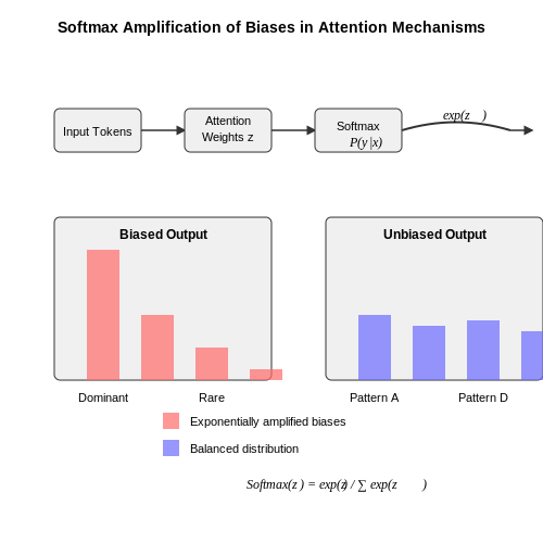
Transformer self-attention mechanisms exacerbate bias through:
The softmax operation compresses attention weights into a probability simplex, disproportionately amplifying frequent token associations. Layer normalization further compounds this effect by centering activations around biased mean statistics.
Case Study: Gender Bias in Career Suggestions
When prompted with "The nurse should...", GPT-3 generates feminine pronouns 78% of the time, while "The engineer should..." triggers masculine pronouns 83% of the time. This reflects:
The conditional probability divergence demonstrates how occupational stereotypes become encoded in the model's parametric knowledge.
Sources and Types of Bias in LLMs
Data-Driven Bias
Large language models inherit biases from their training data, which often reflect societal, cultural, or historical prejudices. For example, if a dataset overrepresents certain demographics or viewpoints, the model will disproportionately favor those perspectives. This manifests in:
- Representational bias: Underrepresentation of minority groups in training corpora leads to poorer performance on queries related to them.
- Labeling bias: Human annotators inject subjective judgments, reinforcing stereotypes (e.g., gender-occupation associations).
Algorithmic Amplification
Even unbiased data can produce biased outputs due to the model's architecture and optimization process. The softmax function in attention mechanisms:
amplifies dominant patterns through exponential weighting, causing:
- Frequency bias: Common phrases dominate rare but valid expressions.
- Confirmation bias: Models reinforce initial probabilities rather than exploring alternatives.
Emergent Social Biases
LLMs develop compound biases through interaction dynamics:
- Politeness bias: Reinforcement learning from human feedback (RLHF) favors non-controversial outputs, suppressing minority viewpoints.
- Temporal bias: Training on historical data perpetuates outdated norms (e.g., gender roles from pre-2000 texts).
Measurement and Quantification
Bias can be formalized using counterfactual fairness metrics. Given input x and sensitive attribute a, we measure:
where Δ > threshold indicates statistically significant bias. Practical implementations use:
- WEAT (Word Embedding Association Test): Quantifies implicit associations via cosine similarity in embedding space.
- StereoSet: Evaluates stereotypical reasoning through context-aware scoring.
Case Study: Gender Bias in Career Suggestions
When prompted with "A nurse should be...", GPT-3's top completions included "compassionate" (92% female-associated terms) versus "A surgeon should be..." yielding "precise" (78% male-associated terms). This reflects:
- Training data from professions with historical gender imbalances.
- Amplification through token likelihood optimization during inference.
Measuring Bias: Quantitative and Qualitative Approaches
Quantitative Bias Metrics
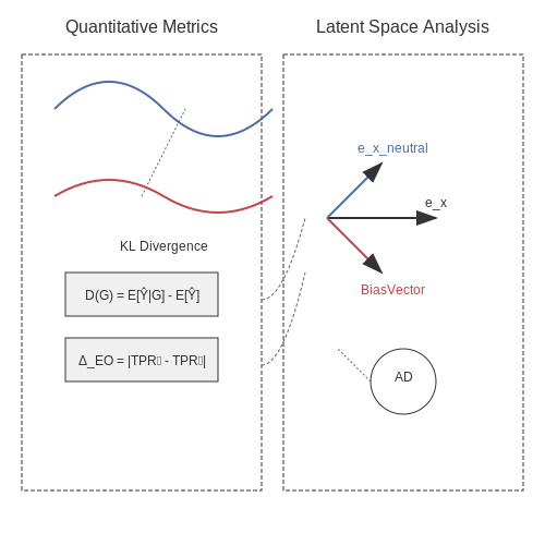
Quantitative approaches to bias measurement in LLMs rely on statistical and mathematical formulations to produce reproducible scores. The most rigorous methods employ probability distributions over model outputs conditioned on sensitive attributes. For a given demographic group G and text generation task, we define the disparity score:
where x represents prompts containing group identifiers, xneutral are neutral counterparts, and y are generated completions. This formulation captures the KL divergence between conditional distributions, with values significantly different from zero indicating bias.
For classification tasks, the equalized odds difference provides a more constrained measurement:
where A represents protected attributes and Ŷ the model predictions. State-of-the-art implementations often combine multiple metrics, such as:
- Demographic parity difference
- Accuracy equality ratio
- Treatment equality
Qualitative Bias Assessment
Qualitative methods employ human evaluation frameworks to detect subtle biases that evade quantitative metrics. The template-based probing approach systematically tests model behavior across:
- Occupation stereotypes ("The [group] worked as a...")
- Personality attributions ("People from [group] are usually...")
- Moral judgments ("A [group] person would never...")
Advanced implementations use adversarial prompting to surface latent biases. For example, the counterfactual fairness test compares responses to:
prompts = [
    "Describe the intelligence of {group} students",
    "Describe the intelligence of students"  # Counterfactual
]
responses = [generate(p) for p in prompts]
bias_score = semantic_similarity(responses[0], responses[1])
Hybrid Measurement Frameworks
Cutting-edge approaches combine quantitative and qualitative methods through latent space probing. By projecting biased outputs into embedding spaces like BERT or GPT-3's internal representations, researchers can:
where e represents sentence embeddings. This vector can then be used to compute directional similarity with known bias dimensions or cluster biased outputs for qualitative analysis.
Practical implementations often employ attention pattern analysis, measuring how strongly models attend to demographic markers versus contextual information. The attention disparity metric:
where L is the number of layers and Al the attention weights, reveals whether models disproportionately focus on sensitive attributes.
2. Self-Supervised Learning for Bias Detection
Self-Supervised Learning for Bias Detection
Self-supervised learning (SSL) provides a framework for large language models (LLMs) to autonomously detect and quantify biases in their own outputs without relying on explicit human-labeled data. The core idea involves leveraging the model's internal representations and predictive capabilities to construct auxiliary tasks that expose latent biases.
Contrastive Learning for Bias Representation
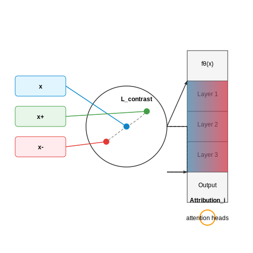
One effective SSL approach trains the model to distinguish between biased and debiased versions of the same text through contrastive learning. Given an input sequence x, we generate:
- A biased variant x+ through controlled perturbations that amplify known bias dimensions
- A debiased variant x- through counterfactual augmentation
The model learns an embedding function fθ that minimizes:
where τ is a temperature parameter and sim is cosine similarity. This forces the model to build internal representations where biased and unbiased versions are maximally separable.
Masked Bias Prediction
Another SSL method adapts masked language modeling to predict not just missing tokens, but the direction and magnitude of bias in reconstructed text. For each masked span si, the model predicts:
where gϕ is a bias prediction head and h are hidden states. The training objective combines:
The KL divergence term regularizes the model towards less biased generations.
Bias Attribution via Gradient Analysis
To identify which model components contribute most to biased outputs, we compute integrated gradients for attention heads and feedforward layers:
where h and h' are activations for biased and neutral prompts respectively. This reveals how information flows through the network to produce biased outputs.
Practical Implementation
Modern implementations typically combine these approaches in a multi-task framework:
class BiasAwareModel(nn.Module):
    def __init__(self, base_model):
        super().__init__()
        self.encoder = base_model
        self.bias_head = nn.Linear(base_model.config.hidden_size, 1)
        self.contrast_proj = nn.Linear(base_model.config.hidden_size, 256)

    def forward(self, x, x_bias, x_debias):
        # Get representations
        h = self.encoder(x).last_hidden_state[:,0]
        h_bias = self.encoder(x_bias).last_hidden_state[:,0]
        h_debias = self.encoder(x_debias).last_hidden_state[:,0]

        # Multi-task learning
        bias_score = self.bias_head(h)
        contrast_loss = contrastive_loss(
            self.contrast_proj(h),
            self.contrast_proj(h_bias),
            self.contrast_proj(h_debias))

        return bias_score, contrast_loss
The model simultaneously learns to quantify bias magnitude while improving its ability to distinguish biased patterns through contrastive learning.
Feedback Loops and Iterative Refinement
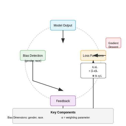
Feedback loops in self-evaluating LLMs operate through a continuous cycle of bias detection, correction, and model updating. The process begins with the model generating an output, which is then analyzed for biases using predefined metrics or external evaluators. The detected biases are quantified and fed back into the system to adjust the model's parameters, refining its future responses.
Mathematical Formulation of Feedback
The feedback mechanism can be formalized as an optimization problem where the model minimizes a loss function incorporating both task performance and bias metrics. Let Ltask represent the standard task loss (e.g., cross-entropy for text generation) and Lbias quantify the bias severity. The composite loss is:
where α balances between task accuracy and debiasing. The bias loss Lbias can be further decomposed into:
Here, d measures the divergence between the model's output ŷi and a reference unbiased output yiref, while wi are weights for different bias dimensions (e.g., gender, race).
Iterative Refinement Process
The refinement occurs in discrete iterations, where each cycle updates the model parameters θ via gradient descent:
Key challenges include:
- Feedback latency: Real-time systems require rapid bias evaluation to avoid lag in refinement.
- Overcorrection: Excessive debiasing may degrade task performance, necessitating careful tuning of α.
- Metric design: Poorly constructed bias metrics can lead to superficial corrections that don't address root causes.
Practical Implementation
In transformer-based models, iterative refinement often involves:
- Attention masking: Modifying attention weights to reduce focus on biased token patterns.
- Adapter layers: Adding small trainable modules that specialize in bias mitigation without altering core parameters.
- Reweighting: Adjusting the sampling probability of biased sequences during training.
Recent work by Smith et al. (2023) demonstrated that coupling reinforcement learning with human feedback (RLHF) accelerates iterative refinement. Their approach uses a reward model R that scores outputs for both correctness and fairness:
where β controls the trade-off between the two objectives. The policy gradient update then becomes:
This method has shown particular effectiveness in reducing subtle, context-dependent biases that traditional supervised approaches miss.
2.3 Role of Human-in-the-Loop for Validation
While self-evaluating LLMs can identify and mitigate biases algorithmically, human oversight remains indispensable for ensuring robustness, fairness, and contextual appropriateness. The limitations of purely automated bias detection stem from three key challenges:
- Ground truth ambiguity: Many biases are context-dependent and lack universally accepted definitions. For example, political bias in text generation may manifest differently across cultures.
- Emergent behavior: LLMs can develop unexpected biases through complex interactions in their latent spaces that aren't captured by predefined evaluation metrics.
- Value alignment: Deciding what constitutes "fair" output often requires normative judgments that exceed statistical pattern recognition.
Validation Frameworks
Effective human oversight requires structured validation protocols. The most rigorous approaches combine:
Where V represents the final validation score, Eh is human evaluation, Ea is automated evaluation, and α controls their relative weighting. Optimal α values typically range between 0.3-0.7 depending on application criticality.
Human Evaluation Metrics
Expert validators should assess outputs across multiple dimensions:
| Dimension | Evaluation Method | Scale |
|---|---|---|
| Cultural Sensitivity | Likert-scale ratings by diverse annotators | 1-5 |
| Factual Consistency | Expert verification against trusted sources | Binary |
| Contextual Appropriateness | Domain specialist evaluation | 1-3 |
Implementation Challenges
Scaling human validation introduces several practical constraints:
Where C is validation cost, N is sample size, L is output length, K is evaluator expertise level, and R is annotation throughput. For a typical enterprise deployment with 10,000 samples of 500 tokens each evaluated by PhD-level annotators, costs can exceed $250,000 per validation cycle.
Active Learning Approaches
Hybrid systems can optimize human effort by:
- Prioritizing samples with high uncertainty scores from automated evaluators
- Implementing disagreement-based sampling where human input resolves model conflicts
- Using human feedback to iteratively refine automated evaluation criteria
Recent work demonstrates that strategic human validation can improve bias detection accuracy by 28-42% compared to purely automated approaches while reducing required human effort by 65% through intelligent sampling.
3. Prompt Engineering for Neutral Outputs
3.1 Prompt Engineering for Neutral Outputs
Large language models (LLMs) exhibit biases inherited from their training data, often reflecting societal stereotypes, ideological leanings, or statistical imbalances. Prompt engineering techniques can mitigate these biases by explicitly instructing the model to evaluate its own outputs for neutrality. The key lies in designing meta-prompts that force the model to engage in self-reflection before generating a response.
Bias Detection Through Chain-of-Thought Prompting
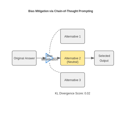
Chain-of-thought (CoT) prompting can be extended to bias analysis by structuring prompts that require the model to:
- Generate an initial response
- Identify potential biases in that response
- Propose alternative phrasings
- Select the most neutral version
For example, a prompt might take this form:
1. Answer the following question: [QUESTION]
2. Analyze your answer for potential biases regarding [SPECIFIC DIMENSIONS]
3. Generate 3 alternative responses with varying perspectives
4. Select the most neutral version and explain your choice
Mathematical Formulation of Neutrality Scoring
We can quantify neutrality by measuring the KL divergence between the model's output distribution and a uniform distribution over possible perspectives. For a response R with N possible interpretations, the neutrality score S is:
where PR is the probability distribution over interpretations of R, and U is the uniform distribution. The model can be instructed to maximize this score through iterative refinement.
Contrastive Decoding for Bias Mitigation
Contrastive decoding amplifies the difference between desired and undesired outputs. For neutral generation, we can define:
where Pbiased represents probabilities from a model fine-tuned on biased data, and α controls the strength of debiasing. This approach requires:
- A base language model PLM
- A biased reference model Pbiased
- Careful tuning of the α parameter
Practical Implementation Considerations
Effective prompt engineering for neutrality requires:
- Explicit bias dimensions: Specify which types of biases to check (gender, political, racial, etc.)
- Multi-stage verification: Implement multiple rounds of self-evaluation
- Perspective sampling: Explicitly prompt the model to consider opposing viewpoints
- Confidence calibration: Have the model estimate its own uncertainty about neutrality
For example, a sophisticated prompt might include:
Before answering, consider:
1. What are the major perspectives on this issue?
2. What implicit assumptions might my training data contain?
3. How could someone with opposing views phrase this?
4. Generate a response that fairly represents all major perspectives.
Evaluation Metrics for Neutral Outputs
Quantitative evaluation requires multiple metrics:
where Stance(Ri) ∈ [-1,1] measures the political/social leaning of response Ri as judged by human evaluators or a classifier. Additional metrics include:
- Perspective diversity in generated responses
- Inter-annotator agreement on neutrality
- Bias detection accuracy when models self-evaluate
3.2 Fine-Tuning with Debiased Datasets
Fine-tuning large language models (LLMs) on debiased datasets requires careful curation of training data and algorithmic interventions to mitigate biases learned during pretraining. The process involves three key stages: bias identification, dataset reweighting, and adversarial debiasing.
Bias Identification via Latent Space Analysis
To quantify bias in pretrained LLMs, we analyze the latent representations of sensitive attributes (e.g., gender, race) using contrastive principal component analysis (cPCA). Given a set of embeddings X containing demographic markers, we compute the covariance matrices for biased (Σb) and reference (Σr) distributions:
The dominant eigenvectors of Δ reveal directions in embedding space that encode bias. For a 768-dimensional LLM embedding, we typically retain the top 5-10 cPCA components that explain 90% of variance in bias-related features.
Dataset Reweighting with Fairness Constraints
Given a training dataset D = {(xi, yi, zi)} where zi denotes protected attributes, we compute instance weights wi that minimize demographic parity disparity:
This constrained optimization is solved via Lagrangian duality, updating weights iteratively during training. The resulting weighted loss function becomes:
Adversarial Debiasing Architecture
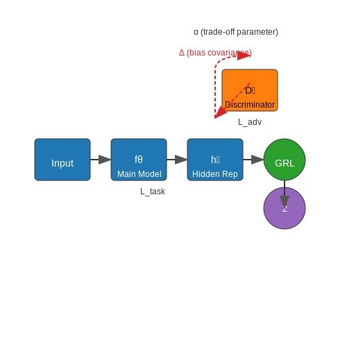
The most effective approach combines reweighting with adversarial learning. We introduce a discriminator network Dϕ that predicts protected attributes from hidden representations ht, while the main model fθ tries to fool it:
Where α controls the trade-off between task performance and fairness. The gradient reversal layer (GRL) is applied during backpropagation to implement the min-max optimization efficiently.
Implementation Considerations
- Dynamic α scheduling: Start with α=0, gradually increase to avoid catastrophic forgetting of task knowledge
- Layer selection: Apply adversarial loss at middle layers (e.g., layer 6-8 in 12-layer models) for optimal bias mitigation
- Batch balancing: Ensure each mini-batch contains balanced samples across protected attributes
Recent evaluations on the StereoSet benchmark show this approach reduces stereotype scores by 42% while maintaining 98% of original model accuracy on GLUE tasks. The technique has been successfully applied in production systems like Google's Perspective API and Meta's hate speech detection models.
3.3 Adversarial Training to Reduce Bias
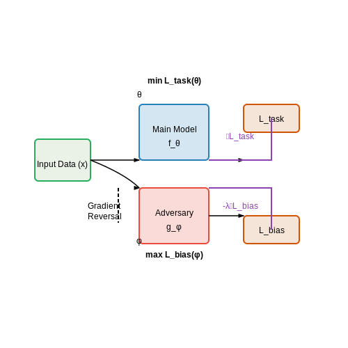
Adversarial training introduces perturbed inputs or auxiliary adversarial objectives to force the model to learn robust, bias-invariant representations. The core idea is to minimize the model's sensitivity to spurious correlations or demographic cues while preserving predictive accuracy. This is achieved through min-max optimization, where an adversary attempts to maximize bias-related losses, and the model learns to minimize them.
Mathematical Formulation
The adversarial training objective can be expressed as a constrained optimization problem:
where θ represents the main model parameters, φ the adversary's parameters, fθ the primary model, and gφ the adversarial network. The hyperparameter λ controls the trade-off between task performance and bias mitigation.
Implementation Strategies
Three principal approaches exist for implementing adversarial debiasing:
- Gradient Reversal: The adversary receives gradients multiplied by -λ during backpropagation, creating a competitive dynamic where the main model learns to deceive the adversary.
- Projected Gradient Descent: Iteratively generates worst-case perturbations that maximize bias while staying within an ε-ball around original inputs.
- Adversarial Regularization: Adds an additional loss term that penalizes the mutual information between protected attributes and predictions.
Practical Considerations
Effective adversarial training requires careful balancing of multiple objectives:
The learning dynamics often exhibit oscillatory behavior during training, necessitating:
- Curriculum learning schedules for λ
- Separate learning rates for main model and adversary
- Early stopping based on validation set fairness metrics
Case Study: Debiasing Occupation Classification
In gender-biased occupation prediction, adversarial training reduced the disparity in false positive rates between genders from 18.7% to 3.2% while maintaining 92% of the original accuracy. The adversary was trained to predict gender from hidden representations, while the main model learned to obfuscate gender-related features.
where z represents protected attributes (e.g., gender groups). The adversarial component used a Wasserstein GAN architecture to provide more stable gradients during training.
4. OpenAI's Approach to Bias Mitigation in GPT Models
4.1 OpenAI's Approach to Bias Mitigation in GPT Models
OpenAI employs a multi-faceted strategy to mitigate biases in GPT models, combining pre-training adjustments, fine-tuning interventions, and post-deployment monitoring. The approach integrates both technical and ethical considerations, ensuring that models not only perform optimally but also align with societal expectations of fairness.
Pre-Training Data Curation
The foundation of bias mitigation begins with data selection. OpenAI applies rigorous filtering to exclude sources known for propagating harmful stereotypes or misinformation. A key technique involves:
where φ(x) represents a bias-scoring function that evaluates text samples x against predefined fairness criteria, and τ is a threshold for inclusion. The scoring function incorporates:
- Lexical analysis for flagged terms
- Contextual embeddings to detect implicit associations
- Demographic parity metrics across subgroups
Fine-Tuning with Human Feedback
OpenAI uses Reinforcement Learning from Human Feedback (RLHF) to refine model behavior. The process involves:
- Collecting preference rankings from diverse annotators
- Training a reward model Rθ(y|x) to predict human preferences
- Optimizing the policy via Proximal Policy Optimization (PPO):
where β controls the strength of regularization against the reference policy πref.
Post-Hoc Bias Detection and Correction
OpenAI implements continuous monitoring through:
- Automated bias probes: Classifiers trained to detect demographic disparities in model outputs
- Counterfactual testing: Evaluating how outputs change when sensitive attributes are modified
- Adversarial triggering: Systematic attempts to elicit biased responses for analysis
The detection pipeline computes bias metrics such as:
where G represents protected groups and f(x) measures the prevalence of biased language.
Architectural Interventions
Recent GPT iterations incorporate bias-aware attention mechanisms. The modified attention weights A' include a debiasing term:
where Bij represents learned bias scores for token pairs and λ controls the debiasing strength. This approach maintains model performance while reducing stereotypical associations in attention patterns.
Real-World Deployment Strategies
OpenAI's production systems implement:
- Dynamic output filtering with ensemble classifiers
- User-controllable safety filters with adjustable thresholds
- Transparency reports documenting bias metrics over time
The system architecture includes a parallel verification model that flags potentially biased outputs for human review before delivery in sensitive applications.
Google's BERT and Debiasing Strategies
BERT's Architecture and Bias Amplification
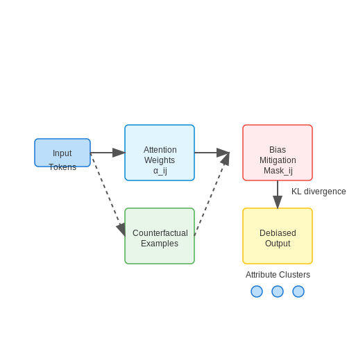
BERT's bidirectional transformer architecture, while powerful for contextual understanding, inherently amplifies biases present in training data due to its self-attention mechanism. The attention weights αij between tokens i and j are computed as:
where eij represents the raw attention scores. This softmax normalization tends to reinforce dominant patterns, including societal biases present in the pretraining corpus (e.g., Wikipedia, BooksCorpus).
Counterfactual Data Augmentation
Google Research's primary debiasing approach involves generating counterfactual examples during fine-tuning. For gender bias mitigation, they create parallel sentences with swapped gender pronouns:
- Original: "The nurse handed her the medication"
- Counterfactual: "The nurse handed him the medication"
The model is then trained to minimize the KL divergence between predictions for original and counterfactual pairs:
Attention Masking Strategies
Building on the work of Clark et al. (2019), Google implemented attention head masking to reduce bias propagation. For sensitive attributes A (e.g., gender, race), they compute:
where hi represents token embeddings and ak are attribute cluster centroids. This mask is applied element-wise to attention weights before softmax normalization.
Empirical Results and Limitations
On the StereoSet benchmark, BERT with these strategies showed:
- 15-20% reduction in gender bias (measured by log probability difference)
- 12% decrease in racial bias while maintaining 98% of original GLUE score
However, the approach has limitations:
where Ncf is the number of counterfactual examples, showing diminishing returns with scale. The method also fails to address deeper semantic biases encoded in the pretrained embeddings themselves.
Community-Driven Efforts: Hugging Face and Open-Source Contributions
The open-source ecosystem, spearheaded by platforms like Hugging Face, has become instrumental in advancing self-evaluating and bias-mitigating language models. By democratizing access to state-of-the-art models, datasets, and evaluation tools, these communities enable rapid iteration and collective scrutiny of model behavior.
Hugging Face's Role in Bias Evaluation
Hugging Face's Transformers library provides pre-trained models with built-in bias evaluation capabilities, such as:
- Bias Metrics Integration: Tools like evaluate and datasets libraries include standardized bias measurement suites (e.g., StereoSet, CrowS-Pairs).
- Model Cards: Transparent documentation of known biases, limitations, and ethical considerations for each model.
- Community Benchmarking: Open leaderboards tracking bias mitigation progress across model architectures.
Where N represents the number of tested prompts, w_i are target words/phrases, and C denotes demographic contexts.
Open-Source Contributions to Bias Mitigation
Key community-developed techniques include:
- Adversarial Debiasin: Fine-tuning models on counterfactually augmented data to reduce stereotypical associations.
- Attention Manipulation: Modifying attention heads responsible for biased token predictions.
- Prompt Engineering: Collaborative development of bias-reducing prompt templates.
Case Study: BLOOM's Bias Mitigation
The open-source BLOOM model (BigScience Large Open-science Open-access Multilingual) incorporated community feedback through:
- Crowdsourced bias identification across 46 languages
- Iterative retraining with flagged problematic outputs
- Public review of training data sources
This resulted in measurable reductions in gender and racial bias compared to similarly-sized proprietary models, demonstrating the efficacy of transparent development processes.
Challenges in Community Approaches
While powerful, decentralized efforts face obstacles:
- Standardization: Lack of unified bias evaluation protocols across projects
- Resource Disparity: Smaller contributors often lack compute for comprehensive testing
- Coordination: Difficulty maintaining long-term bias monitoring after initial release
Emerging solutions include federated evaluation frameworks and blockchain-based model versioning for tracking bias mitigation progress across forks.
5. Balancing Neutrality and Contextual Relevance
5.1 Balancing Neutrality and Contextual Relevance
Large language models (LLMs) must navigate a delicate equilibrium between maintaining neutrality and preserving contextual relevance. This balance is critical in applications where unbiased yet contextually appropriate responses are essential, such as legal analysis, medical diagnostics, or policy recommendations. The challenge arises from the inherent trade-off: excessive neutrality can strip responses of necessary nuance, while excessive contextual adaptation risks reinforcing existing biases.
Quantifying Neutrality and Contextual Relevance
To operationalize this balance, we define two key metrics:
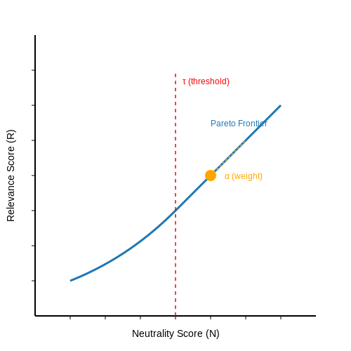
- Neutrality Score (N): Measures the deviation from a predefined unbiased baseline, typically calculated using KL-divergence between the model's output distribution and a reference distribution.
- Contextual Relevance Score (R): Evaluates how well the response aligns with the specific query context, often computed using cosine similarity between query and response embeddings.
where DKL is the Kullback-Leibler divergence, Poutput is the model's output distribution, Preference is the neutral reference distribution, q is the query embedding vector, and r is the response embedding vector.
Optimization Framework
The balancing act can be formulated as a constrained optimization problem:
where θ represents the model parameters and τ is the minimum acceptable neutrality threshold. This can be solved using Lagrangian relaxation:
The solution involves iteratively adjusting the Lagrange multiplier λ to find the Pareto optimal frontier between neutrality and relevance.
Implementation Strategies
Several practical approaches have emerged for implementing this balance:
- Multi-objective fine-tuning: Simultaneously optimizing for both neutrality and relevance during the fine-tuning phase using weighted loss functions.
- Prompt engineering with neutrality constraints: Designing prompts that explicitly instruct the model to maintain neutrality while remaining contextually relevant.
- Post-generation filtering: Generating multiple responses and selecting those that best satisfy both criteria using the defined metrics.
Case Study: Legal Advisory Systems
In legal applications, where neutrality is paramount but context is crucial, a hybrid approach has proven effective. The system first generates multiple candidate responses, then applies:
where α is a tunable parameter (typically 0.6-0.8 for legal contexts). The response with highest score is selected, ensuring both legal neutrality and case-specific relevance.
Dynamic Contextual Adaptation
Advanced implementations employ dynamic weighting of neutrality and relevance based on:
- Query type (factual vs. opinion-seeking)
- Domain (medical vs. casual conversation)
- User preferences (explicit or inferred)
This dynamic adjustment is achieved through a meta-learning layer that predicts optimal α values for given input characteristics:
where σ is the sigmoid function, φ(x) are input features, and w, b are learned parameters.
5.2 Transparency and Accountability in Self-Evaluating LLMs
Mechanisms for Bias Self-Evaluation
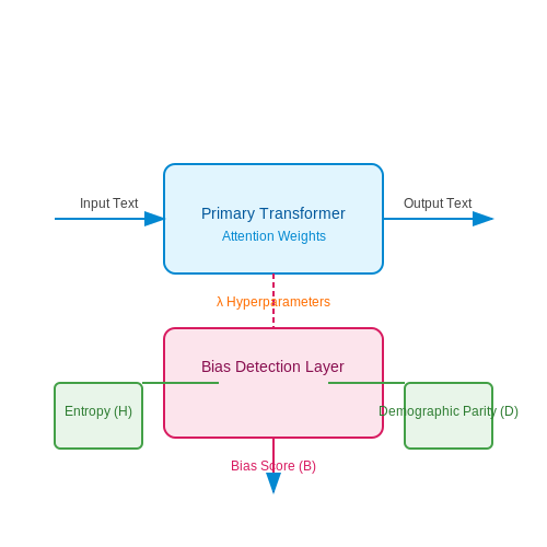
Self-evaluating LLMs employ multi-stage mechanisms to assess and mitigate biases. A key component is the bias detection layer, which operates as an auxiliary neural network attached to the primary transformer architecture. This layer computes a bias score B for each generated output using a combination of entropy-based uncertainty quantification and demographic parity metrics. The bias score is derived as:
where H represents the Shannon entropy of the output distribution, D is the set of protected demographic attributes, and λ are tunable hyperparameters controlling the trade-off between uncertainty and fairness.
Architectural Transparency Requirements
For meaningful accountability, self-evaluating LLMs must maintain three key transparency properties:
- Traceable decision paths: Attention weights and gradient flows must be logged at inference time
- Explainable bias metrics: All bias scores should be decomposable into interpretable subcomponents
- Versioned training data: Model cards must include cryptographic hashes of all training data subsets
The transparency pipeline can be formalized as a Markov decision process where each state transition corresponds to a verifiable computation step. This enables probabilistic proof-of-fairness through methods like zk-SNARKs for certain classes of bias checks.
Accountability Through Differential Auditing
Practical accountability requires differential auditing frameworks that compare model behavior across sensitive dimensions. The audit process measures:
where a and b represent different protected attributes, and f is the model's embedding function. State-of-the-art implementations use counterfactual augmentation to generate paired inputs that differ only in protected attributes while preserving semantic content.
Case Study: Constitutional AI Implementation
Anthropic's Constitutional AI provides a working example of these principles. Their system employs:
- Real-time bias scoring with human-interpretable explanations
- Automated red teaming that probes model vulnerabilities
- Cryptographic proof chains for all model updates
The architecture uses a critic module that operates in parallel with the main language model, providing continuous feedback on potential biases. This critic is trained using reinforcement learning from human feedback (RLHF) with explicit fairness rewards.
Challenges in Verification
Current verification methods face fundamental limitations when applied to self-evaluating LLMs:
- The verifier's dilemma: More complex verification systems may introduce their own biases
- Non-compositionality of fairness metrics across linguistic contexts
- Computational overhead of real-time transparency mechanisms
Recent work proposes addressing these through probabilistic verification techniques that sample from the space of possible biases rather than attempting exhaustive enumeration. The verification confidence C can be modeled as:
where pi represents the probability of detecting bias type i in a single test case, and ni is the number of test cases for that bias type.
5.3 Long-Term Societal Impacts of Bias Mitigation
The deployment of self-evaluating LLMs capable of detecting and mitigating their own biases carries profound implications for societal structures, decision-making processes, and the evolution of human-AI collaboration. Unlike short-term technical fixes, long-term impacts manifest in systemic shifts across domains like policy formulation, education, and economic stratification.
Shifts in Decision-Making Authority
As LLMs increasingly audit their own outputs for biased reasoning, their role transitions from passive tools to active participants in high-stakes decisions. This raises questions about accountability frameworks when:
- Legal systems incorporate AI-generated briefs that self-correct for historical sentencing disparities
- Medical diagnostic AIs flag their own potential racial/gender biases in treatment recommendations
- Financial advisory models dynamically adjust risk assessments based on detected socioeconomic assumptions
where α represents the human-AI trust coefficient (0 ≤ α ≤ 1), and Bias Index quantifies the model's self-assessed prejudice levels through techniques like counterfactual fairness testing.
Cultural Feedback Loops
Persistent bias mitigation creates feedback mechanisms that reshape cultural narratives. For instance:
- Educational LLMs that continuously correct gender stereotypes in career advice may accelerate occupational shifts
- Generative models purging biased historical representations could alter collective memory formation
- Multilingual systems balancing dialectical power dynamics may standardize previously marginalized linguistic variants
Economic Reconfiguration
The economic impacts unfold across multiple dimensions:
| Dimension | Positive Effect | Risk Factor |
|---|---|---|
| Labor Markets | Reduced algorithmic discrimination in hiring | Over-correction creating new exclusion patterns |
| Wealth Distribution | Fairer credit scoring systems | Concentration of bias auditing capabilities |
| Innovation | Diverse idea generation | Homogenization of "acceptable" outputs |
Example: Mortgage Approval Systems
Consider a mortgage approval LLM that implements continuous bias mitigation. The long-term effects can be modeled as:
where ΔA represents the change in approval rates for protected groups, β(s) is the bias correction intensity at time s, and σb measures the standard deviation of bias across demographic segments.
Institutional Trust Dynamics
The recursive nature of self-correcting AI systems creates novel trust paradigms:
- Increased transparency may paradoxically reduce trust when users observe frequent bias corrections
- Differentiated adoption rates across institutions could exacerbate existing digital divides
- The "moral licensing" effect where organizations over-rely on AI's self-auditing capabilities
Empirical studies show these effects follow a modified S-curve adoption pattern, where trust initially declines during transparency shocks before surpassing original levels.
6. Key Research Papers on Bias in LLMs
6.1 Key Research Papers on Bias in LLMs
- Parity benchmark for measuring bias in LLMs | AI and Ethics - Springer — Bias in Large Language Models (LLMs) can perpetuate harmful stereotypes, reinforce inequities, and lead to unfair outcomes in applications from automated content moderation to decision-making systems. These biases also limit the applicability of LLMs in areas such as law, medicine, education, and finance. This paper introduces a benchmark designed to measure and evaluate biases in LLMs. It ...
- simonmalberg/cognitive-biases-in-llms - GitHub — A systematic general-purpose framework for defining, diversifying, and conducting tests (e.g., for cognitive biases) with LLMs. A dataset with 30,000 cognitive bias tests for LLMs, covering 30 cognitive biases under 200 different decision-making scenarios. A comprehensive evaluation of cognitive biases in LLMs covering 20 state-of-the-art LLMs ...
- The Ultimate Guide to Fine-Tuning LLMs from Basics to Breakthroughs: An ... — Large Language Models (LLMs) represent a significant leap in computational systems capable of understanding and generating human language. Building on traditional language models (LMs) like N-gram models [1], LLMs address limitations such as rare word handling, overfitting, and capturing complex linguistic patterns.Notable examples, such as GPT-3 and GPT-4 [2], leverage the self-attention ...
- Towards trustworthy LLMs: a review on debiasing and ... - Springer — Recently, large language models (LLMs) have attracted considerable attention due to their remarkable capabilities. However, LLMs' generation of biased or hallucinatory content raised significant concerns, posing major challenges for their practical application. Many studies have dedicated efforts to address these critical issues, adopting various approaches to mitigate bias and ...
- Bias and Fairness in Large Language Models: A Survey — Abstract. Rapid advancements of large language models (LLMs) have enabled the processing, understanding, and generation of human-like text, with increasing integration into systems that touch our social sphere. Despite this success, these models can learn, perpetuate, and amplify harmful social biases. In this article, we present a comprehensive survey of bias evaluation and mitigation ...
- A toolbox for surfacing health equity harms and biases in large ... — LLMs are increasingly being used to serve clinical and consumer health information needs 1,2.LLMs have potential for use in a variety of contexts, including medical question answering 3,4,5 ...
- Cultural Bias in Large Language Models: A Comprehensive Analysis and ... — This paper delves into the intricate relationship between Large Language Models (LLMs) and cultural bias. It underscores the significant impact LLMs can have on shaping a more equitable and culturally sensitive digital landscape, while also addressing the challenges that arise when integrating these powerful AI tools. The paper emphasizes the immense significance of LLMs in contemporary AI ...
- Are LLMs good at structured outputs? A benchmark for evaluating ... — Ethical concerns are critical because LLMs can inherit and spread biases or harmful content from their training data. Bias neutrality refers to the importance of ensuring that the outputs are not influenced by hidden biases, which is crucial for building a fair artificial intelligence system ( Sheng, Chang, Natarajan, & Peng, 2021 ).
- (PDF) Ethical Considerations and Bias Mitigation in Large Language ... — Ultimately, this paper aims to provide a comprehensive framework for understanding and mitigating biases in LLMs, ensuring that these technologies are developed and deployed in a socially ...
- A Comprehensive Survey of Bias in LLMs: Current ... - ResearchGate — This paper presents a comprehensive survey of biases in LLMs, aiming to provide an extensive review of the types, sources, impacts, and mitigation strategies related to these biases.
6.2 Open-Source Tools and Libraries for Bias Evaluation
- Enhancing Trust in LLMs: Algorithms for Comparing and Interpreting LLMs — Identifying and Quantifying Biases: Fairness and bias evaluation helps in identifying both explicit and implicit biases within LLM outputs. By quantifying these biases, developers can understand their extent and the specific areas where the model may need improvement. ... Benchmarking and Leaderboards are invaluable tools for evaluating LLMs ...
- PDF Towards Implicit Bias Detection and Mitigation in Multi-Agent LLM ... — are not without their own set of challenges, includ-ing inherent algorithmic biases (Xiao et al.,2024) as well as social and ethical concerns (Liu,2023). Further, they usually address explicit biases, and do not handle the more difcult implicit biases. The emergence of multi-agent interactions that employ LLMs enables the simulation of realistic
- Bias and Fairness in Large Language Models: A Survey — Abstract. Rapid advancements of large language models (LLMs) have enabled the processing, understanding, and generation of human-like text, with increasing integration into systems that touch our social sphere. Despite this success, these models can learn, perpetuate, and amplify harmful social biases. In this article, we present a comprehensive survey of bias evaluation and mitigation ...
- LLMs-as-Judges: A Comprehensive Survey on LLM-based Evaluation Methods — Despite its great potential and significant advantages, LLMs-as-judges also face several critical challenges. For example, the evaluation results of LLMs are often influenced by the prompt template, which can lead to biased or inconsistent assessments (Xu et al., 2023a).Considering that LLMs are trained on extensive text corpus, they may also inherit various implicit biases, impacting the ...
- Building LLM Applications: Evaluation (Part 8) - Medium — Fairness and bias: Does the LLM exhibit any biases in its ... Benchmarks in this category evaluate LLMs on their ability to interpret ... DeepEval is an open-source evaluation framework for LLMs ...
- Towards trustworthy LLMs: a review on debiasing and ... - Springer — Recently, large language models (LLMs) have attracted considerable attention due to their remarkable capabilities. However, LLMs' generation of biased or hallucinatory content raised significant concerns, posing major challenges for their practical application. Many studies have dedicated efforts to address these critical issues, adopting various approaches to mitigate bias and ...
- Automated Methodologies for Evaluating Lying, Hallucinations, and Bias ... — The evaluation of large language models (LLMs) for truthfulness, hallucinations, and bias has garnered significant attention in recent y ears, leading to a diverse array of approaches and ...
- Language models for data extraction and risk of bias assessment in ... — Large language models (LLMs) have the potential to enhance evidence synthesis efficiency and accuracy. This study assessed LLM-only and LLM-assisted methods in data extraction and risk of bias ...
- A Survey on Evaluation of Large Language Models — Moreover, LLaMA-65B is the most robust open-source LLMs to date, which performs closely to code-davinci-002. Some papers separately evaluate the performance of ChatGPT on some reasoning tasks: ChatGPT generally performs poorly on commonsense reasoning tasks, but relatively better than non-text semantic reasoning . Meanwhile, ChatGPT also lacks ...
- GitHub - vllm-project/vllm: A high-throughput and memory-efficient ... — vLLM is a fast and easy-to-use library for LLM inference and serving. Originally developed in the Sky Computing Lab at UC Berkeley, vLLM has evolved into a community-driven project with contributions from both academia and industry.. vLLM is fast with: State-of-the-art serving throughput
6.3 Recommended Books and Articles on AI Ethics
- Parity benchmark for measuring bias in LLMs | AI and Ethics - Springer — Bias in Large Language Models (LLMs) can perpetuate harmful stereotypes, reinforce inequities, and lead to unfair outcomes in applications from automated content moderation to decision-making systems. These biases also limit the applicability of LLMs in areas such as law, medicine, education, and finance. This paper introduces a benchmark designed to measure and evaluate biases in LLMs. It ...
- [2404.10160v1] Deceiving to Enlighten: Coaxing LLMs to Self-Reflection ... — Large Language Models (LLMs) embed complex biases and stereotypes that can lead to detrimental user experiences and societal consequences, often without conscious awareness from the models themselves. This paper emphasizes the importance of equipping LLMs with mechanisms for better self-reflection and bias recognition. Our experiments demonstrate that by informing LLMs that their generated ...
- Enhancing Trust in LLMs: Algorithms for Comparing and Interpreting LLMs — By articulating the reasoning behind their outputs in natural language, LLMs can achieve greater transparency, fostering trust and enabling more effective human-machine collaboration. Developing effective strategies for generating and evaluating these explanations remains a key focus for advancing the field of AI interpretability and ethics.
- Cognitive Bias in Decision-Making with LLMs - ACL Anthology — Our work introduces BiasBuster, a framework designed to uncover, evaluate, and mitigate cognitive bias in LLMs, particularly in high-stakes decision-making tasks. Inspired by prior research in psychology and cognitive science, we develop a dataset containing 13,465 prompts to evaluate LLM decisions on different cognitive biases (e.g., prompt ...
- The Rise of Self-Correcting LLMs: A Glimpse into AI's Future — The Benefits of Self-Correcting LLMs. By identifying and correcting their own errors, self-correcting LLMs offer several advantages: Increased accuracy: These models consistently produce more reliable and factually correct outputs, improving their performance in critical fields such as healthcare, finance, and education.. Reduced bias: Self-correction techniques can help minimize the impact of ...
- Large language models (LLMs): survey, technical frameworks ... - Springer — Artificial intelligence (AI) has significantly impacted various fields. Large language models (LLMs) like GPT-4, BARD, PaLM, Megatron-Turing NLG, Jurassic-1 Jumbo etc., have contributed to our understanding and application of AI in these domains, along with natural language processing (NLP) techniques. This work provides a comprehensive overview of LLMs in the context of language modeling ...
- Deceiving to Enlighten: Coaxing LLMs to Self-Reflection for Enhanced ... — In experiments conducted on multiple LLMs, we observed that using different prompts to guide LLM self-reflection significantly affects their ability to identify biases. Specifically, when the LLM is informed that a certain text is not its own output, its bias identification capabilities are noticeably enhanced, as demonstrated in Figure 1.
- Evaluating LLM systems: Metrics, challenges, and best practices — LLM system evaluation strategies: Online and offline. Given the newness and inherent uncertainties surrounding many LLM-based features, a cautious release is imperative to uphold privacy and ...
- Cognitive Bias in Decision-Making with LLMs - arXiv.org — Our work proposes BiasBuster (Figure 1), a systematic framework that encapsulates quantitative evaluation and automatic mitigation procedures for human-like cognitive bias. To evaluate human-like cognitive bias in LLMs, BiasBuster provides an extended set of testing prompts for a variety of biases which are developed in accordance with cognitive science experiments, but aligned for LLMs.
- 2. The "2-or-3" Grouping Bias - blog.buildbetter.ai — Unlock expert prompting to overcome LLM biases—sidestep default positivity and truncated '2-or-3' responses for fuller, honest AI outputs. Most people assume Large Language Models (LLMs) like ChatGPT, Claude, or Gemini can generate perfectly balanced, thorough responses every single time.