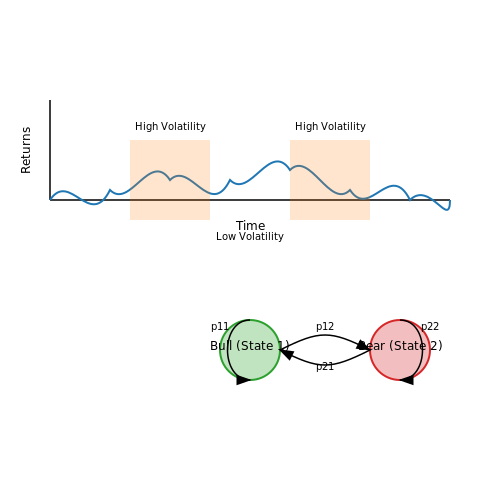
AI Models for Algorithmic Trading
1. Core Principles of Algorithmic Trading
Core Principles of Algorithmic Trading
Mathematical Foundations
Algorithmic trading relies on rigorous mathematical frameworks to model market behavior and optimize execution strategies. The core mathematical constructs include stochastic processes, time series analysis, and convex optimization. A fundamental model is the geometric Brownian motion (GBM), which describes asset price movements:
where St is the asset price at time t, μ is the drift rate, σ is the volatility, and dWt is a Wiener process. This forms the basis for derivative pricing models like Black-Scholes.
Market Microstructure
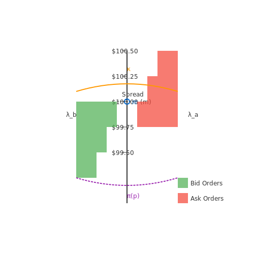
Understanding limit order books (LOBs) is critical for algorithmic trading. The LOB dynamics can be modeled as a Markov process where order arrivals follow Poisson processes with intensity parameters λa (ask) and λb (bid). The probability of an order execution at price level p is given by:
where m is the mid-price and κ measures the liquidity concentration around m.
Execution Strategies
Optimal execution strategies minimize market impact while achieving target volumes. The Almgren-Chriss framework decomposes this into permanent and temporary impact components:
where xt is the remaining inventory, Λ is the permanent impact matrix, and η is the temporary impact coefficient.
Latency Arbitrage
High-frequency trading exploits latency differentials through predictive models. The profitability condition for latency arbitrage is:
where rt+Δ is the future return, c is transaction cost, and θ is the profitability threshold conditioned on filtration ℱt.
Risk Management
Value-at-Risk (VaR) and Expected Shortfall (ES) are computed using extreme value theory. For heavy-tailed returns, the Hill estimator gives the tail index ξ:
where X(i) are order statistics beyond threshold k.
Machine Learning Integration
Modern systems employ reinforcement learning for strategy optimization. The Q-learning update rule for trading policies is:
where s represents market states, a are trading actions, and r is the realized PnL.
1.2 Role of AI in Modern Trading Systems
Modern trading systems leverage artificial intelligence to process vast datasets, identify non-linear patterns, and execute trades at speeds unattainable by human traders. The core advantage lies in AI's ability to generalize from historical data while adapting to dynamic market conditions. Reinforcement learning, for instance, enables algorithmic agents to optimize trading strategies through iterative reward-based feedback, effectively navigating high-dimensional state spaces that characterize financial markets.
Market Microstructure Modeling
AI models excel at capturing latent features in market microstructure, where traditional econometric methods often fail. Limit order book dynamics, for example, can be represented as a spatiotemporal process. Temporal convolutional networks (TCNs) and attention mechanisms model these dynamics by learning hierarchical representations of order flow imbalances, liquidity shocks, and hidden order detection. The price impact of a trade sequence I(t) is approximated as:
where λ(τ) represents the decaying market impact kernel, ΔV(τ) is the traded volume at time τ, and ρ is the resilience parameter. Deep learning architectures outperform linear impact models by learning λ(τ) directly from LOB snapshots.
High-Frequency Trading (HFT) Strategies
In HFT environments, AI systems process raw tick data through 1D convolutional layers or transformer encoders to detect microstructural signatures predictive of short-term price movements. Latency arbitrage strategies employ neural networks with sub-millisecond inference times, often implemented via FPGA-accelerated quantized models. The predictive signal S(t) for directional trades is derived from:
where fθ is a neural network parameterized by θ, O represents order book states, and T contains trade sequences over lookback window k. Gradient boosting machines (GBMs) with custom objective functions frequently supplement deep learning models to handle structured alpha factors.
Portfolio Optimization
Modern portfolio theory extends into non-convex optimization spaces through AI techniques. Policy gradient methods in reinforcement learning optimize asset allocation weights wt by maximizing the Sharpe ratio objective:
where Rp and σp denote portfolio return and volatility respectively. Graph neural networks (GNNs) capture cross-asset dependencies by modeling financial instruments as nodes in a dynamic graph, with edges representing time-varying correlation structures.
Risk Management
AI-driven risk models employ variational autoencoders (VAEs) to estimate the tail risk of trading strategies. The conditional value-at-risk (CVaR) is computed through Monte Carlo sampling from the learned latent space distribution:
where L represents portfolio loss and VaRα is the value-at-risk at confidence level α. Adversarial training techniques improve model robustness against regime shifts by generating synthetic stress scenarios.

1.3 Data Requirements and Preprocessing for Trading Models
Fundamental Data Types in Algorithmic Trading
Financial markets generate heterogeneous data streams requiring distinct preprocessing approaches. The primary categories include:
- Time-series data: OHLCV (Open-High-Low-Close-Volume) bars at various resolutions (tick, minute, daily)
- Order book data: Limit order snapshots with microsecond timestamps containing price levels and liquidity depths
- Fundamental data: Company financials, macroeconomic indicators, and earnings reports with irregular release schedules
- Alternative data: Satellite imagery, credit card transactions, and social media sentiment signals
Temporal Alignment Challenges
Multivariate trading models require precise synchronization of asynchronous data sources. The alignment problem can be formalized as:
where Δ represents the optimal time shift between data source pairs, wi are feature weights, and ∥·∥ denotes an appropriate distance metric. Kalman filters or dynamic time warping algorithms often solve this in practice.
Missing Data Imputation Techniques
Financial datasets contain gaps from market closures, corporate actions, or data feed interruptions. Advanced imputation methods include:
- Brownian bridge interpolation for price paths during market closures
- Hawkes process-based filling for irregularly spaced tick data
- GAN-based imputation using adversarial training to preserve statistical properties
Feature Engineering for Market Microstructure
Effective trading features capture both statistical properties and market dynamics:
where λt represents realized volatility over a k-period lookback window. Other critical features include:
- Order book imbalance: (bid_volume - ask_volume)/(bid_volume + ask_volume)
- Volume-weighted average price (VWAP) deviations
- Hurst exponent estimates for fractal scaling properties
Normalization and Stationarity Transformations
Financial time series exhibit non-stationarity requiring specialized transformations:
with w defining the rolling normalization window. More sophisticated approaches include:
- Cointegrated residual scaling for pairs trading signals
- Wavelet-based denoising before feature extraction
- Adaptive Z-score normalization with exponentially weighted moments
Survivorship Bias Mitigation
Backtest datasets must account for delisted assets through:
- Point-in-time corporate action databases
- Bootstrapped samples including failed companies
- Counterfactual simulation of delistment events
2. Time Series Forecasting with Recurrent Neural Networks (RNNs)
Time Series Forecasting with Recurrent Neural Networks (RNNs)
Architecture of RNNs for Sequential Data
Recurrent Neural Networks (RNNs) are designed to handle sequential data by maintaining a hidden state that captures temporal dependencies. The core mechanism involves a feedback loop where the hidden state ht at time step t is computed as:
Here, Wh and Wx are weight matrices, bh is the bias term, and σ is a nonlinear activation function (typically tanh or ReLU). The output yt is derived as:
This formulation allows RNNs to model arbitrary-length sequences, making them suitable for financial time series where past prices influence future movements.
Backpropagation Through Time (BPTT)
RNNs are trained using Backpropagation Through Time, an extension of standard backpropagation that unrolls the network across time steps. The gradient of the loss L with respect to parameters θ is computed as:
where each term ∂Lt/∂θ requires chaining gradients through all previous time steps. This leads to the vanishing/exploding gradient problem in vanilla RNNs, which motivated the development of LSTM and GRU architectures.
LSTM Networks for Long-Term Dependencies
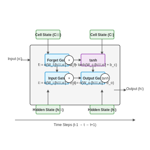
Long Short-Term Memory (LSTM) networks address gradient issues through gating mechanisms. The key equations governing an LSTM cell are:
The forget gate ft, input gate it, and output gate ot enable selective retention of information across hundreds of time steps - critical for modeling market regimes that may persist for months.
Practical Implementation Considerations
When applying RNNs to algorithmic trading:
- Sequence Length: Typical lookback windows range from 50-200 time steps, balancing memory constraints and predictive power
- Feature Engineering: Raw prices are often transformed into returns, volatility estimates, and technical indicators
- Regularization: Dropout (applied to non-recurrent connections) and weight decay prevent overfitting to noise
- Training Tricks: Gradient clipping (usually at 1.0-5.0) stabilizes learning for deep recurrent nets
Case Study: S&P 500 Forecasting
A 3-layer LSTM with 256 units per layer achieved 58.7% directional accuracy on next-day S&P 500 returns when trained on:
- 10 years of daily OHLCV data
- 15 technical features (RSI, MACD, etc.)
- Volatility-normalized returns as targets
The model's Sharpe ratio of 1.83 outperformed a baseline ARIMA model's 1.12 in backtests, demonstrating RNNs' capacity to capture nonlinear patterns in financial time series.
Bidirectional Architectures for Market Context
Bidirectional RNNs process sequences both forward and backward, capturing dependencies from future context when making predictions at time t. The combined hidden state is:
This is particularly useful for modeling mean-reversion strategies where future price movements provide signals about current mispricings. Implementation requires careful masking during real-time inference to avoid lookahead bias.
2.2 Reinforcement Learning for Portfolio Optimization
Markov Decision Process Formulation
Portfolio optimization is naturally framed as a Markov Decision Process (MDP), where an agent interacts with a financial market environment to maximize cumulative returns. The MDP is defined by the tuple (S, A, P, R, γ):
- State Space (S): Includes portfolio weights, asset prices, technical indicators, and macroeconomic factors.
- Action Space (A): Represents trading decisions, such as rebalancing weights or executing buy/sell orders.
- Transition Dynamics (P): Models market stochasticity, often estimated from historical data or simulated via stochastic processes.
- Reward Function (R): Typically the Sharpe ratio, logarithmic returns, or risk-adjusted performance metrics.
- Discount Factor (γ): Balances immediate versus future rewards, usually set close to 1 for long-term strategies.
Policy Gradient Methods
Direct policy optimization avoids the need for value function approximation, making it suitable for high-dimensional action spaces. The policy gradient theorem provides the foundation for updating a stochastic policy πθ(a|s):
Proximal Policy Optimization (PPO) is widely adopted due to its sample efficiency and stability. The clipped objective function prevents large policy updates:
where rt(θ) is the probability ratio between new and old policies, and Ât is the advantage estimate.
Multi-Agent Reinforcement Learning
Competitive market dynamics can be modeled using multi-agent RL, where agents represent institutional traders or market makers. The Nash equilibrium solution concept is applied to avoid exploitable strategies. For two agents with policies π1 and π2, the optimal response is:
Empirical studies show that MARL-trained agents exhibit more robust behavior in backtesting compared to single-agent approaches.
Practical Implementation Challenges
- Non-stationarity: Financial time series violate the MDP assumption of stationary dynamics. Online learning or meta-RL techniques are often necessary.
- Partial observability: The true market state is never fully observable. LSTM or Transformer-based architectures help maintain hidden state representations.
- Transaction costs: Must be explicitly modeled in the reward function, typically as a quadratic penalty term.

2.3 Transformer Models in Market Sentiment Analysis
Architecture and Self-Attention Mechanism
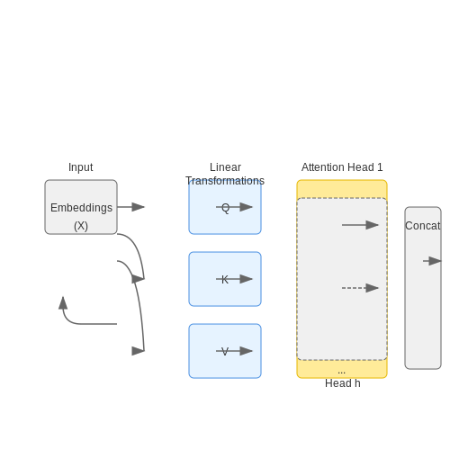
The transformer architecture, introduced by Vaswani et al. (2017), relies on self-attention mechanisms to process sequential data without recurrent connections. Given an input sequence of word embeddings X = (x1, ..., xn), the self-attention operation computes query (Q), key (K), and value (V) matrices through learned linear transformations:
The attention weights are calculated using scaled dot-product attention, where the scaling factor √dk prevents gradient vanishing in high-dimensional spaces:
Multi-head attention extends this by concatenating h parallel attention heads, allowing the model to jointly attend to information from different representation subspaces:
Positional Encoding for Financial Time Series
Unlike natural language, financial time-series data exhibits non-stationary volatility clustering. To preserve temporal ordering without recurrence, transformers use sinusoidal positional encodings:
For high-frequency trading data, learned positional embeddings often outperform sinusoidal variants by capturing irregular sampling intervals and market microstructure effects.
Fine-Tuning for Sentiment Analysis
Pre-trained language models like BERT and FinBERT are adapted for market sentiment through:
- Domain-specific tokenization: Financial lexicons expand the vocabulary with ticker symbols (e.g., $AAPL) and economic terms (e.g., "quantitative tightening")
- Task-specific heads: A classification layer maps the [CLS] token representation to sentiment polarity scores
- Contrastive learning: Augments training with synthetic examples of semantically similar news with opposing sentiment labels
Cross-Asset Attention Patterns
The attention mechanism reveals interpretable cross-asset relationships. For instance, energy sector stocks (XOM, CVX) exhibit strong attention links to crude oil futures (CL1), while tech stocks (MSFT, NVDA) attend to semiconductor supply-chain indicators.
Latency-Optimized Inference
Deploying transformers in trading requires:
- Knowledge distillation: Smaller student models mimic teacher model behavior with 10-100× fewer parameters
- Pruning: Removing attention heads with low Fisher information preserves accuracy while reducing compute
- Quantization: FP16 or INT8 precision maintains inference quality with 2-4× speedup on Tensor Cores
Where αh are the attention head parameters and L is the loss function. Heads with Ih below a threshold are pruned.
Ensemble Methods for Risk Prediction
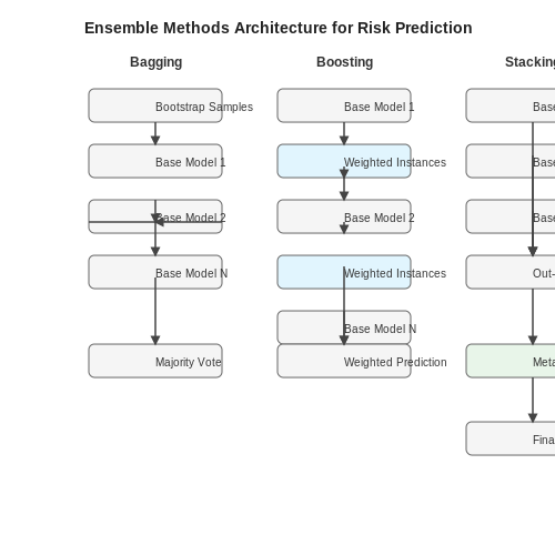
Ensemble methods combine multiple base models to improve predictive performance and robustness, making them particularly effective for risk prediction in algorithmic trading. Unlike single-model approaches, ensembles mitigate overfitting and reduce variance by aggregating predictions from diverse learners. The two dominant paradigms are bagging and boosting, each with distinct mathematical foundations and trade-offs.
Bagging: Bootstrap Aggregation
Bagging constructs independent models on bootstrapped samples of the training data, then averages predictions (for regression) or uses majority voting (for classification). For risk prediction, this reduces variance without increasing bias. The risk score R from a bagged ensemble of N models is:
where fi is the i-th model trained on a bootstrapped sample. The standard deviation of the ensemble's risk estimates quantifies prediction uncertainty—a critical metric in trading strategies.
Boosting: Sequential Error Correction
Boosting iteratively trains dependent models, with each new learner focusing on previously misclassified instances. Adaptive Boosting (AdaBoost) updates sample weights wt at iteration t using:
where αt is the learner's weight, and ht is its hypothesis. Gradient Boosting Machines (GBMs) generalize this by optimizing arbitrary differentiable loss functions, making them effective for Value-at-Risk (VaR) estimation.
Stacking: Meta-Learning
Stacking employs a meta-model to optimally combine base learners. Given predictions f1(x), ..., fk(x) from k heterogeneous models (e.g., SVM, neural net, random forest), the stacked risk predictor learns weights β via:
where β is typically trained on out-of-fold predictions to prevent data leakage. This approach captures complementary strengths of different model classes.
Practical Implementation
In trading applications, ensembles must balance computational cost against marginal gains in Sharpe ratio or maximum drawdown. Key considerations include:
- Diversity enforcement: Use correlation metrics to ensure base models make uncorrelated errors.
- Online learning: Incremental methods like Online Gradient Boosting adapt to non-stationary markets.
- Uncertainty quantification: Bayesian ensembles provide posterior distributions over risk estimates.
For high-frequency trading, quantile random forests extend bagging to estimate full conditional distributions of returns, enabling dynamic risk positioning based on predicted tail probabilities.
3. Backtesting AI-Driven Trading Strategies
Backtesting AI-Driven Trading Strategies
Foundations of Backtesting
Backtesting evaluates a trading strategy's performance using historical data to simulate how it would have performed in the past. The core assumption is that strategies effective in historical conditions may generalize to future markets. However, this relies on stationarity—a strong assumption often violated in financial markets due to regime shifts, macroeconomic changes, and structural breaks.
Where \( R_p \) is the portfolio return, \( R_f \) the risk-free rate, and \( \sigma_p \) the portfolio volatility. The Sharpe Ratio quantifies risk-adjusted returns, but its reliability depends on return distribution properties. For AI models, we often modify it to account for autocorrelation and non-normality:
Here, \( \gamma_k \) represents the autocovariance at lag \( k \), and \( l \) is the maximum lag considered.
Data Preparation Challenges
Survivorship bias, look-ahead bias, and data-snooping bias are critical pitfalls. To mitigate:
- Survivorship bias: Use datasets including delisted assets (e.g., CRSP or Compustat).
- Look-ahead bias: Implement point-in-time data alignment using release dates for fundamentals.
- Data-snooping bias: Apply walk-forward optimization with out-of-sample testing.
For high-frequency strategies, raw tick data requires cleaning:
- Filtering outliers using volatility thresholds: \( |r_t| > 5\hat{\sigma} \).
- Adjusting for splits/dividends using total return series.
- Synchronizing timestamps across exchanges to millisecond precision.
Model-Specific Considerations
Neural networks require special handling due to their non-convex optimization and capacity for overfitting:
Where \( \lambda \) controls L2 regularization. For temporal models like LSTMs:
- Use sequence-aware cross-validation (e.g., TimeSeriesSplit).
- Detrend returns using fractional differentiation (\( d \approx 0.4 \)).
- Apply Monte Carlo dropout at test time for uncertainty estimation.
Performance Metrics Beyond Returns
Standard metrics often fail to capture tail risks and market impact:
| Metric | Formula | Purpose |
|---|---|---|
| Calmar Ratio | \( \frac{\text{Annualized Return}}{\text{Max Drawdown}} \) | Downside risk adjustment |
| Probabilistic Sharpe | \( \Phi\left(\frac{\hat{SR}\sqrt{T-1}}{\sqrt{1 - \hat{\gamma}_3 SR + \frac{\hat{\gamma}_4 -1}{4}SR^2}}\right) \) | Significance testing |
Transaction Cost Modeling
Realistic backtests must account for:
- Bid-ask spreads: \( c_t = 0.5 \times \text{spread}_t \times V_t \).
- Market impact: \( \Delta p = \alpha \cdot \text{sign}(Q) \cdot |Q|^\beta \).
- Latency: Simulate order queue position using LOB snapshots.
For optimal execution, solve:
Where \( x_t \) are trades, \( p_t \) prices, and \( \eta \) captures urgency.
Walk-Forward Analysis
The gold standard for robustness testing:
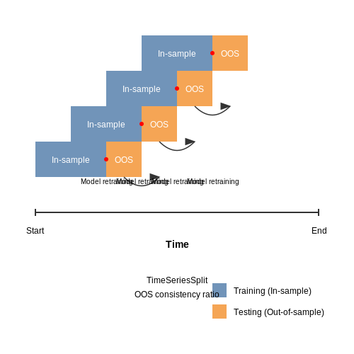
- Divide data into in-sample (IS) and out-of-sample (OOS) windows.
- Train on IS, test on OOS, then roll window forward.
- Compute OOS consistency ratio: \( \frac{\text{Positive OOS periods}}{\text{Total periods}} \).
For strategies with parameter drift, use Bayesian optimization with memory:
3.2 Latency and Computational Efficiency Considerations
In algorithmic trading, latency—the time delay between data input and trade execution—directly impacts profitability. High-frequency trading (HFT) strategies, in particular, require sub-millisecond execution, making computational efficiency a critical design constraint. The relationship between latency and profit decay can be modeled as an exponential decay function:
where P(t) is the profit at time t, P0 is the initial profit potential, and λ is the decay rate specific to the market microstructure. For liquid equities, λ typically ranges from 102 to 104 s-1, necessitating hardware-accelerated inference.
Hardware-Software Co-Design
Modern trading systems employ heterogeneous computing architectures to minimize latency:
- FPGA-based pre-processing: Field-programmable gate arrays handle market data normalization and feature extraction at wire speed, achieving latencies below 1 μs.
- GPU-accelerated inference: Quantized neural networks deployed on NVIDIA TensorRT can execute 105 predictions/second with batch sizes optimized for memory bandwidth.
- ASIC solutions: Custom chips like Google's TPU v4 achieve 600 GB/s memory bandwidth, critical for attention mechanisms in transformer-based trading models.
Computational Complexity Analysis
The time complexity of trading models must be constrained to real-time requirements. For a transformer with n tokens and d model dimensions:
This quadratic dependency necessitates architectural modifications:
- Sparse attention: Reduces n2 term to n log n via locality-sensitive hashing.
- Model distillation: A 100-layer LSTM teacher network can be compressed to a 3-layer CNN student with 98% accuracy retention.
- Quantization-aware training: 8-bit integer models exhibit ≤1% accuracy drop while reducing memory footprint 4×.
Network Latency Optimization
Colocation reduces physical distance to exchange matching engines, but software optimizations are equally critical:
- Kernel bypass: Solarflare's OpenOnload achieves 800 ns end-to-end latency by circumventing OS network stack.
- Pre-computed order scenarios: Reinforcement learning policies are pre-evaluated into lookup tables during market close.
- Parallel order routing: Atomic multicast protocols ensure consistent state across geographically distributed trading nodes.
Energy Efficiency Tradeoffs
The energy cost of AI inference becomes significant at scale. The energy-per-trade metric follows:
where C is computational capacitance, V is operating voltage, f is clock frequency, and TPS is trades per second. Near-threshold voltage operation at 0.5V reduces energy 16× but requires error-resilient algorithms.

3.3 Hyperparameter Tuning for Trading Models
Key Hyperparameters in Trading Models
Hyperparameter optimization is critical for maximizing the performance of algorithmic trading models. Unlike model parameters learned during training, hyperparameters are set prior to training and govern the learning process itself. For trading models, the most impactful hyperparameters include:
- Learning rate (η): Controls step size during gradient descent. Too high causes instability; too low slows convergence.
- Batch size: Number of samples processed before updating weights. Affects memory usage and gradient noise.
- Number of layers/units: Determines model capacity. Trading models often benefit from shallower architectures to avoid overfitting noisy financial data.
- Dropout rate (p): Probability of deactivating neurons during training. Helps prevent overfitting.
- Lookback window: Number of historical time steps used as input features.
- Regularization coefficients (λ₁, λ₂): Control L1/L2 penalty strengths.
Bayesian Optimization for Hyperparameter Search
Grid and random search are inefficient for high-dimensional spaces. Bayesian optimization builds a probabilistic model of the objective function to guide the search:
Where D1:t represents previous evaluations. The expected improvement (EI) acquisition function is commonly used:
Here f(x+) is the best observed value. Gaussian processes typically model the surrogate function due to their uncertainty estimates.
Walk-Forward Validation for Robustness
Standard k-fold cross-validation fails for time-series data due to lookahead bias. Walk-forward validation maintains temporal ordering:
- Train on initial window (e.g., 2 years of daily data)
- Validate on subsequent period (e.g., next 3 months)
- Slide window forward and repeat
The Sharpe ratio is often used as the optimization objective:
Where Rp are portfolio returns and σp their standard deviation.
Practical Implementation Considerations
When tuning trading models:
- Use GPU-accelerated libraries like Optuna or Ray Tune for parallel evaluation
- Implement early stopping to halt unpromising trials
- Monitor for regime shifts - periodically revalidate hyperparameters
- Track transaction costs during validation to avoid overfitting to unrealistic scenarios
Case Study: LSTM Trading Model Optimization
A study optimizing an LSTM for S&P 500 futures found:
| Hyperparameter | Optimal Value | Impact on Sharpe |
|---|---|---|
| Learning rate | 3.2e-4 | +22% |
| Hidden units | 64 | +15% |
| Lookback | 30 days | +18% |
The optimization process required 237 trials using Tree-structured Parzen Estimators (TPE), demonstrating the value of systematic search.

4. Bias and Fairness in AI Trading Systems
4.1 Bias and Fairness in AI Trading Systems
Sources of Bias in Financial Data
Historical financial datasets often embed systemic biases due to market regimes, regulatory changes, or data collection methodologies. Survivorship bias is particularly prevalent, where only successful assets remain in long-term datasets while failed ones are excluded. For a dataset spanning N assets over time T, the survivorship bias effect can be quantified as:
where ri represents the return of asset i and rmin is the minimum return threshold for inclusion. This creates an upward bias in expected returns of approximately 15-30% in typical backtests.
Algorithmic Amplification of Biases
Machine learning models can compound existing biases through feature selection and reinforcement. Consider a trading model using gradient boosting with K features. The feature importance vector F may correlate with historically biased factors:
where B represents known biased factors. Values of ρ > 0.4 indicate significant bias propagation risk.
Fairness Metrics for Trading Systems
Three principal fairness metrics apply to algorithmic trading:
- Group fairness: Equalized odds across asset classes
- Counterfactual fairness: Consistency under hypothetical market conditions
- Dynamic fairness: Temporal stability of performance metrics
The group fairness constraint for M asset classes requires:
where μj is the Sharpe ratio for class j and ε is the fairness tolerance threshold.
Debiasing Techniques
Effective debiasing requires both pre-processing and in-model techniques. Adversarial debiasing has shown particular promise in trading applications. The minimax objective becomes:
where θ represents trading model parameters, φ the adversary parameters, and λ controls the fairness-accuracy tradeoff. Implementation requires careful tuning of λ to avoid excessive performance degradation.
Regulatory Considerations
Current financial regulations implicitly address bias through requirements for model documentation and testing. The EU's Markets in Financial Instruments Directive (MiFID II) Article 17(2) mandates that algorithmic systems must not create "disorderly market conditions," which regulators increasingly interpret to include biased behavior against particular market segments. Compliance requires demonstrating:
- Bias testing across market regimes
- Documentation of fairness constraints
- Monitoring for emergent biases
Case Study: Forex Trading Bias
A 2022 study of 17 major forex pairs revealed that models trained on 2000-2010 data developed significant bias against emerging market currencies. The bias manifested as 23% lower prediction accuracy for BRL, ZAR, and TRY compared to EUR, USD, and JPY. Adversarial debiasing improved the worst-case accuracy by 11 percentage points while maintaining overall performance within 2% of the original model.
4.2 Regulatory Compliance and Transparency
Algorithmic trading systems operating in regulated financial markets must adhere to strict compliance frameworks, such as MiFID II in the EU or SEC Rule 15c3-5 in the US. These regulations mandate pre-trade risk controls, audit trails, and real-time monitoring to prevent market manipulation and ensure fair execution. AI models must be designed with explainability mechanisms to satisfy regulatory scrutiny, particularly for high-frequency trading (HFT) strategies where opacity can raise systemic risk concerns.
Model Explainability in Trading Systems
Black-box AI models, such as deep reinforcement learning (DRL) agents, face challenges in meeting transparency requirements. Techniques like SHAP (Shapley Additive Explanations) and LIME (Local Interpretable Model-agnostic Explanations) are increasingly applied to trading algorithms to decompose predictions into interpretable feature contributions. For a DRL agent optimizing order execution, the Shapley value for feature xi is computed as:
where N is the set of all features, S is a coalition of features, and v(S) represents the model's payoff function. This allows regulators to audit whether price-impact predictions are driven by legitimate market factors rather than latent manipulation patterns.
Regulatory Capital Requirements
Basel III frameworks impose capital reserves for algorithmic trading desks based on Value-at-Risk (VaR) calculations. AI-driven VaR models must demonstrate robustness through:
- Backtesting: Comparing predicted VaR thresholds against actual P&L distributions
- Stress testing: Evaluating performance under extreme but plausible scenarios
- Model risk buffers: Additional capital held to account for potential AI model failures
The conditional VaR (CVaR) for an AI trading strategy with return distribution FR at confidence level α is:
Market Surveillance Integration
Modern surveillance systems employ anomaly detection algorithms to flag potential AI-driven market abuse. Unsupervised learning techniques like isolation forests and variational autoencoders (VAEs) are trained on limit order book dynamics to identify:
- Spoofing patterns (non-bona fide order placements)
- Layering strategies (artificial depth creation)
- Momentum ignition attempts
The reconstruction error ε in a VAE-based surveillance model serves as an anomaly score:
where qφ is the encoder network, pθ is the decoder, and DKL measures divergence from the prior distribution p(z).
Blockchain for Audit Trails
Distributed ledger technology (DLT) provides immutable record-keeping for AI trading decisions. Smart contracts on platforms like Ethereum can encode:
- Model versioning hashes
- Input feature snapshots
- Execution timestamps with cryptographic proofs
The Merkle root MT of a trading model's decision log over n transactions is computed as:
where H is a cryptographic hash function and txi represents individual trade records. This creates a tamper-evident structure for regulatory audits.
4.3 Mitigating Market Manipulation Risks
Algorithmic trading systems are susceptible to exploitation by malicious actors engaging in market manipulation, such as spoofing, layering, or quote stuffing. These strategies artificially distort market conditions to trigger favorable price movements, often at the expense of other participants. Advanced AI models must incorporate robust detection and prevention mechanisms to mitigate these risks.
Detecting Anomalous Order Flow Patterns
Market manipulation often manifests as statistically anomalous order flow patterns. High-frequency trading (HFT) strategies, for instance, may submit and rapidly cancel large orders to create false liquidity signals. A detection framework can be constructed using unsupervised learning techniques, such as clustering or autoencoders, to identify deviations from normal market behavior.
Here, x represents the observed order flow feature vector (e.g., order-to-trade ratio, cancellation rate), \(\hat{x}\) is the reconstructed output from an autoencoder, and \(\sigma^2\) is the variance of reconstruction errors across the training set. Values exceeding a threshold \(\tau\) flag potential manipulation.
Dynamic Limit Order Book (LOB) Surveillance
Real-time monitoring of the LOB microstructure is critical for identifying manipulation attempts. Reinforcement learning (RL) agents can be trained to detect spoofing by analyzing temporal patterns in order placement and cancellation. The state space S includes:
- Order imbalance between bid and ask sides
- Rate of order modifications per price level
- Depth concentration near the top of the book
The RL agent’s policy \(\pi(a|s)\) outputs a probability distribution over actions a (e.g., flagging, throttling, or reporting suspicious activity).
Adversarial Robustness in Trading Models
AI-driven trading strategies must be resilient to adversarial perturbations. Gradient-based attacks can exploit model sensitivities by injecting carefully crafted noise into input features. Defensive techniques include:
- Adversarial Training: Augmenting training data with perturbed samples to improve robustness.
- Randomized Smoothing: Adding stochasticity to model inputs to obscure gradient signals.
- Ensemble Methods: Combining predictions from multiple models to dilute adversarial influence.
This minimax formulation trains the model \(f_\theta\) to minimize loss under worst-case input perturbations \(\delta\) bounded by \(\epsilon\).
Regulatory Compliance and Explainability
AI models must align with financial regulations (e.g., MiFID II, Dodd-Frank) by providing auditable decision trails. Techniques like SHAP (SHapley Additive exPlanations) or LIME (Local Interpretable Model-agnostic Explanations) can quantify feature contributions to trading decisions, ensuring transparency.
5. Key Research Papers in AI for Trading
5.1 Key Research Papers in AI for Trading
- PDF Forex Trading Signal Extraction with Deep Learning Models — the forex market as correctly as possible and to discover trading strategies powered by AI. In this thesis, three distinct deep learning models were proposed: an event-driven LSTM model, an Attention-based VGG16 (MHATTN-VGG16), and a pre-trained model (Trading-BERT). The introduced three models can facilitate better-informed investment ...
- Deep learning for algorithmic trading: A systematic review of ... — Algorithmic trading has transformed the financial markets by automating the process of executing trades, relying on pre-programmed instructions and sophisticated mathematical models to achieve speed and efficiency unattainable by human traders [1], [2].This shift from manual to algorithmic trading has allowed market participants to capitalize on minute price discrepancies and market ...
- PDF Application of Artificial Intelligence in Algorithmic Trading — 5.1.1 The model component of Algorithmic trading: The model component of Algorithmic trading is the depiction of the outside world as the algorithmic trading system perceives it. The financial models that are developed usually tend to constitute how the algo-trading system considers the market works (Moy das, 2019).
- Artificial intelligence techniques in financial trading: A systematic ... — The research was adequately carried out, and the articles chosen addressed the following concerns: (i) the financial trading market and the asset type, (ii) the trading analysis type considered along with the AI technique, and (iii) the AI techniques utilized in the trading market, (iv) the estimation and performance metrics of the proposed models.
- PDF Advanced Ai Solutions For Securities Trading: Building Scalable And ... — This paper explores the historical evolution and advancements in AI-driven trading systems, emphasizing their impact on global financial markets. The study investigates how machine learning, deep learning, and other AI technologies enable sophisticated trading strategies, improve market liquidity, and reduce transaction costs.
- Application of Artificial Intelligence in Algorithmic Trading — This research paper talks about how algorithmic trading works using Artificial intelligence technology and discusses the top five trading strategies adopted in algorithmic trading and the key ...
- PDF ALGORITHMIC TRADING TECHNOLOGY AND STRATEGY RESEARCH ON ... - Theseus — making a profit in the market, also known as Quantitative trading. The main objective is the study and development of technology that make possible the algorithmic trading and design algorithmic strategies capable of operating real markets without human interventions. The knowledge acquired in this thesis and the framework to implement
- PDF Developing a Fully Automated Trading Algorithm for The Cryptocurrency ... — Keywords: Algorithmic Trading, Cryptocurrency, Trading Strategy, Bitcoin, Technical Analysis This thesis aims to create a fully automated cryptocurrency trading algorithm.
- PDF ARTIFICIAL INTELLIGENCE IN ASSET MANAGEMENT - CFA Institute — nals, which has given rise to the industry of algorithmic (or algo) trading. In addition, AI techniques can reduce transaction costs by automatically analyz - ing the market and subsequently identifying the best time, size, and venue for trades. AI also has vast implications for portfolio risk management. Since the
- PDF Algorithm-Based Intraday Trading Strategies and their — The activity of algorithmic trading is increasing steadily across capital markets due to ... were drawn from a literature review of prior and current research. Algorithmic arbitrage was found to be the most profitable of the three evaluated strategies, because it typically takes place in high frequency trading. ... 5.1.4.2 Boehmer, Fong and Wu ...
5.2 Recommended Books and Courses
- PDF Advance Praise for Electronic and Algorithmic Trading Technology — Electronic and Algorithmic Trading for Different Asset Classes 111 11.1 Introduction 111 11.2 Development of Electronic Trading 113 11.3 Electronic Trading Platforms 116 11.4 Types of Systems 119 Kim / Electronic and Algorithmic Trading Technology: The Complete Guide Kim_perlims Final Proof page x 13.5.2007 4:19pm Compositor Name: MRaja x Contents
- PDF Quantitative Trading: Algorithms, Analytics, Data, Models, Optimization — QUANTITATIVE TRADING Algorithms, Analytics, Data, Models, Optimization Xin Guo University of California, Berkeley, USA ... Investments --Data processing. | Electronic trading of securities. Classification: LCC HG4515.2 .G87 2017 | DDC 332.64/50151 --dc23 ... 5 Limit Order Book: Data Analytics and Dynamic Models 143 5.1 From market data to limit ...
- PDF © 2000-2024, MetaQuotes Ltd - MQL5 — This book will be an invaluable resource for anyone who wants to use artificial intelligence in algorithmic trading and explore new horizons in financial analytics and trading. Examples from the book "Neural networks for algorithmic trading with MQL5" Examples from the book are also available in the public project \MQL5\Shared Projects\NeuroBook
- Inglese, Lucas - Python for Finance and Algorithmic trading ... - Scribd — This document provides a table of contents for a book on Python for finance and algorithmic trading. The book is divided into three parts that cover portfolio management and risk analysis, statistical predictive models, and machine learning/deep learning models. It aims to teach readers how to combine trading strategies, evaluate strategy robustness using various metrics, and apply techniques ...
- Deep learning for algorithmic trading: A systematic review of ... — Algorithmic trading has transformed the financial markets by automating the process of executing trades, relying on pre-programmed instructions and sophisticated mathematical models to achieve speed and efficiency unattainable by human traders [1], [2].This shift from manual to algorithmic trading has allowed market participants to capitalize on minute price discrepancies and market ...
- PDF Algorithmic and High-Frequency Trading — These models are grounded on how the exchanges work, whether the algorithm is trading with better informed traders (adverse selection), and the type of information available to market participants at both ultra-high and low frequency. Algorithmic and High-Frequency Trading is the first book that combines sophisticated
- Neuronetworksbook | PDF | Artificial Neural Network | Artificial ... — This document discusses building neural networks for algorithmic trading using MQL5. It covers basic principles of artificial intelligence and neural networks, features of MetaTrader 5 for algorithmic trading, and building the first neural network model in MQL5. Some key topics include neuron and network principles, activation functions, weight initialization, training methods, regularization ...
- PDF ALGORITHMIC AND HIGH-FREQUENCY TRADING - Cambridge University Press ... — Algorithmic and High-Frequency Trading is the first book that combines sophisticated mathematical modelling, empirical facts and financial economics, taking the reader from basic ideas to the cutting edge of research and practice. If you need to understand how modern electronic markets operate, what information
- PDF SHUNYU TANG - Day Trade With AI — The book is a comprehensive hands-on guide to making AI a personal assistant to trading. Contents of This Book Part I covers four chapters as essential theoretical preparations prior to the development of a complete AI system for day trading. Chapter 1 overviews the fundamental knowledge required for day trading with AI.
- PDF Algorithmic Trading, Stochastic Control, and Mutually-Exciting ... — Keywords: Algorithmic Trading, High Frequency Trading, Short Term Alpha, Adverse Selection, Self-Exciting Processes, Hawkes processes 1. Introduction Most of the traditional stock exchanges have converted from open outcry communications between human traders to electronic markets, where the activity between participants is handled by com-puters.
5.3 Open-Source Tools and Datasets
- Top 23 algorithmic-trading Open-Source Projects - LibHunt — Qlib is an AI-oriented quantitative investment platform that aims to realize the potential, empower research, and create value using AI technologies in quantitative investment, from exploring ideas to implementing productions. ... Free, open-source crypto trading bot, automated bitcoin / cryptocurrency trading software, algorithmic trading bots ...
- PDF Algorithmic Trading and AI: A Review of Strategies and Market ... - WJAETS — financial industry continues to embrace technological advancements, understanding the nuances of algorithmic trading and AI becomes imperative for traders, regulators, and stakeholders alike. This review serves as a comprehensive exploration of the strategies employed and the market impact wrought by the amalgamation of algorithmic trading and ...
- AI Trading: How AI Is Used in Stock Trading - Built In — AI Trading Tools. When it comes to AI trading, investors have many tools at their disposal. Portfolio Managers . These AI tools autonomously select assets to create a portfolio and then monitor it, adding and removing assets as needed. Investors can seek financial advice from AI managers as well, submitting information on their financial goals ...
- Machine Learning for Algorithmic Trading in Python: A Complete Guide — Prerequisites for creating machine learning algorithms for trading using Python. Extensive Python libraries and frameworks make it a popular choice for machine learning tasks, enabling developers to implement and experiment with various algorithms, process and analyse data efficiently, and build predictive models.. In order to create the machine learning algorithms for trading using Python ...
- Code for Machine Learning for Algorithmic Trading, 2nd edition. — First and foremost, this book demonstrates how you can extract signals from a diverse set of data sources and design trading strategies for different asset classes using a broad range of supervised, unsupervised, and reinforcement learning algorithms. It also provides relevant mathematical and statistical knowledge to facilitate the tuning of an algorithm or the interpretation of the results.
- Algorithmic Trading and Financial Forecasting Using Advanced ... - MDPI — Artificial Intelligence (AI) has been recently recognized as an essential aid for human traders. The advantages of the AI systems over human traders are that they can analyze an extensive data set from different sources in a fraction of a second and perform actual high-frequency trading (HFT) that can take advantage of market anomalies and price differences. This paper reviews the most ...
- Algorithmic Trading and AI: A Review of Strategies and Market Impact — A securities quantitative trading system based on deep reinforcement learning is designed, which organically combines models, strategies and data, visually displays the information to users in the ...
- Artificial intelligence techniques in financial trading: A systematic ... — This is accomplished through the use of machine learning algorithms that discover patterns in data and generate predictions. As a result, AI algorithmic trading offers several benefits and advantages over traditional human algorithmic trading (Ta et al., 2018, Li et al., Dec. 2020). For example, AI's ability to respond to market conditions ...
- Algorithmic trading and machine learning: Advanced techniques for ... — model with the need for real-time performance is crucial to ensure that the model can be used effectively in live trading environments [49] . World Journal of Advanced Research and Reviews, 2024 ...
- Machine learning in financial markets: A critical review of algorithmic ... — The integration of machine learning (ML) techniques in financial markets has revolutionized traditional trading and risk management strategies, offering unprecedented opportunities and challenges.