Analyzing Call Center Audio for Insights
1. Key Components of Call Center Audio Data
Key Components of Call Center Audio Data
Raw Audio Waveforms
The fundamental representation of call center audio is the raw waveform, typically sampled at 8 kHz for telephony applications. The waveform x(t) is a time-domain signal where amplitude variations encode acoustic pressure changes. For digital processing, the continuous signal is discretized using pulse-code modulation (PCM) with µ-law or A-law companding to optimize dynamic range:
where Q(·) denotes quantization, μ = 255 for North American telephony standards, and n represents discrete time indices. The 8 kHz sampling rate preserves frequencies up to 4 kHz, sufficient for speech intelligibility while minimizing bandwidth.
Mel-Frequency Cepstral Coefficients (MFCCs)
MFCCs remain the dominant feature representation for speech analysis, derived through:
- Framing the waveform into 20-40 ms segments with 10 ms overlap
- Computing the power spectrum via Short-Time Fourier Transform (STFT)
- Applying mel-scale filter banks to approximate human auditory perception
- Taking the discrete cosine transform (DCT) of log filterbank energies
where E(m) is the energy in the mth mel filter and c[n] are the cepstral coefficients. Typically, the first 13 coefficients capture vocal tract characteristics while higher-order coefficients encode excitation sources.
Speaker Diarization Features
Call center audio requires robust speaker separation. Beyond MFCCs, additional features include:
- Pitch (F0): Computed via autocorrelation or cepstral analysis to identify vocal fold vibration frequency
- Spectral centroid: Measures the "center of mass" of the power spectrum, indicating voice brightness
- Voice activity detection (VAD): Uses Gaussian mixture models (GMMs) on energy and spectral flux to segment speech from silence
Linguistic Content
Transcribed text from automatic speech recognition (ASR) systems provides semantic analysis opportunities. Key representations include:
where wt are word tokens generated by transformer-based ASR models like Whisper or Conformer. The word error rate (WER) in call centers typically ranges 5-15% depending on acoustic conditions.
Paralinguistic Features
Non-verbal cues contain critical emotional and behavioral information:
- Jitter and shimmer: Micro-variations in pitch and amplitude indicating stress
- Speaking rate: Syllables per second computed via forced alignment
- Pause patterns: Distribution of inter-utterance silences
These features are particularly valuable for sentiment analysis and agent performance evaluation. For example, increased jitter (σ > 0.5%) correlates with customer frustration at p < 0.01 significance in controlled studies.
Acoustic Environment Characteristics
Call quality metrics must account for transmission artifacts:
where Perceptual Evaluation of Speech Quality (PESQ) scores range 1 (bad) to 4.5 (excellent). Modern systems use neural networks to predict MOS-LQO (Mean Opinion Score - Listening Quality Objective) from spectral features.

Common Use Cases for Audio Analysis in Call Centers
Sentiment and Emotion Recognition
Advanced audio analysis pipelines leverage deep learning architectures like convolutional neural networks (CNNs) and transformer-based models to extract paralinguistic features from speech signals. These models analyze spectral characteristics (MFCCs, spectrograms) and prosodic features (pitch, intensity, speaking rate) to classify emotional states. A typical implementation involves:
where f represents the fused feature vector, S is the spectrogram input, and P contains prosodic features. State-of-the-art systems achieve >85% accuracy in valence-arousal classification when trained on benchmark datasets like IEMOCAP.
Automated Quality Assurance
Neural speech-to-text systems coupled with attention mechanisms enable real-time monitoring of agent performance metrics:
- Script adherence scoring using BERT-based semantic similarity
- Compliance detection through keyword spotting with finite state transducers
- Conversation analytics via hierarchical dialogue act classification
The system architecture typically employs a multi-task learning framework where shared encoder layers process the audio stream before task-specific heads generate quality scores.
Speaker Diarization and Separation
Modern diarization systems combine x-vector embeddings with spectral clustering to resolve the permutation problem in overlapping speech. The key technical components include:
where PLDA performs probabilistic linear discriminant analysis on deep features extracted by a TDNN network. Recent advancements like end-to-end neural diarization (EEND) further improve performance through self-attention mechanisms.
Real-Time Voice Analytics
Streaming architectures deploy causal convolutional networks with bounded latency for live call monitoring. The technical implementation requires:
- Frame-wise processing with look-ahead constraints (<100ms)
- Incremental feature extraction using sliding window DFT
- Dynamic batching for GPU-optimized inference
Edge deployment considerations include quantized models (INT8 precision) and hardware-accelerated MFCC extraction using DSP pipelines.
Fraud Detection and Security
Audio forensics techniques identify synthetic speech and spoofing attacks through:
- Spectro-temporal artifact detection using linear frequency cepstral coefficients (LFCC)
- Neural vocoder fingerprinting with residual networks
- Anti-spoofing countermeasures from ASVspoof challenge baselines
The detection pipeline typically computes a bonafide score through a ensemble of specialized classifiers operating on complementary feature representations.
1.3 Challenges in Processing Call Center Audio
Acoustic Variability and Noise
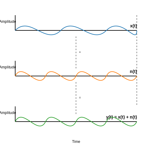
Call center audio exhibits significant acoustic variability due to factors such as background noise, varying microphone quality, and speaker accents. The signal-to-noise ratio (SNR) is often low, complicating speech recognition and sentiment analysis. Background noise can be modeled as additive Gaussian noise:
where x(t) is the clean speech signal and n(t) represents noise. Traditional denoising techniques like spectral subtraction or Wiener filtering struggle with non-stationary noise sources common in call centers (e.g., keyboard typing, overlapping speech).
Speaker Diarization Complexity
Accurately segmenting audio into speaker turns (diarization) is challenging due to:
- Overlapping speech: Agents and customers frequently interrupt each other.
- Short utterances: Many responses are brief (e.g., "yes", "no"), providing insufficient data for voiceprint analysis.
- Channel effects: Telephone networks apply bandwidth limiting (typically 300-3400 Hz), removing discriminative high-frequency features.
State-of-the-art diarization systems use neural embeddings (e.g., x-vectors) with clustering, but performance degrades when:
where D is the distance between speaker clusters and σ is the within-speaker variance.
Emotion Recognition Limitations
Extracting emotional states from audio faces three key hurdles:
- Cultural variability: Prosodic patterns signaling anger or happiness differ across dialects.
- Paralinguistic cues: Sighs, pauses, and laughter carry meaning but lack standardized representations.
- Data imbalance: Most call center datasets are dominated by neutral tones, causing classifiers to underperform on rare emotional extremes.
Current approaches fuse acoustic features (e.g., MFCCs, pitch contours) with lexical analysis, but achieve only 60-70% accuracy in real-world deployments.
Compliance and Privacy Constraints
Processing call center audio must address:
- GDPR/CCPA requirements: Speaker anonymization while preserving linguistic content.
- Selective redaction: Removing payment card information or other sensitive data without disrupting flow analysis.
- Storage limitations: High-resolution audio demands compression that maintains analytic utility.
Differential privacy techniques are increasingly applied to acoustic feature extraction, adding controlled noise to embeddings:
where β controls the privacy-utility tradeoff.
Real-Time Processing Demands
Live analysis requires:
- Low-latency ASR: End-to-end delays under 500ms to avoid agent-customer disruption.
- Streaming architectures: Windowed processing of infinite audio streams without full conversation context.
- Hardware constraints:
- CPU/GPU limitations in on-premise call centers
- Network bandwidth for cloud processing
Modern systems use hybrid models where lightweight edge devices perform initial feature extraction, while cloud servers handle complex analytics.
2. Methods for Capturing and Storing Call Audio
Methods for Capturing and Storing Call Audio
Audio Capture Techniques
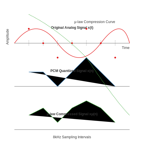
Call center audio is typically captured using telephony systems that convert analog voice signals into digital form. The most common approach involves pulse-code modulation (PCM), which samples the audio signal at a fixed rate. For telephony applications, the Nyquist-Shannon sampling theorem dictates a minimum sampling rate of 8 kHz to capture frequencies up to 4 kHz, the standard bandwidth for voice communications. The quantization process typically uses 8-bit μ-law or A-law companding to optimize dynamic range while maintaining acceptable signal-to-noise ratios.
where x(n) represents the normalized input signal, μ is the compression parameter (typically 255 for North American systems), and sgn() denotes the sign function.
Digital Storage Formats
Captured audio is stored in various digital formats, each with distinct advantages:
- WAV (Waveform Audio File Format): Uncompressed PCM audio, preserving maximum fidelity at the cost of storage space (typically 64 kbps for 8 kHz, 8-bit mono)
- MP3: Lossy compression achieving 8-16 kbps rates through psychoacoustic modeling, sacrificing some high-frequency content
- Opus: Hybrid codec combining SILK for speech and CELT for music, supporting variable bitrates from 6 kbps to 510 kbps
- G.711: Standard PCM codec used in traditional telephony systems (64 kbps)
Streaming vs. Batch Processing
Modern call centers implement either:
- Real-time streaming: Audio is processed as it's captured, with minimal latency (typically <100ms). Requires robust network infrastructure and distributed processing frameworks like Apache Kafka or WebRTC.
- Batch processing: Calls are recorded in full before analysis, allowing for more computationally intensive processing. Typically stored in cloud object storage (AWS S3, Azure Blob) with metadata tagging.
Metadata Synchronization
Each audio recording must be associated with rich metadata for subsequent analysis:
where τsync measures the synchronization error between audio timestamps tiaudio and corresponding log entries tilog across N events.
Storage Architecture
Large-scale call centers require distributed storage architectures:
- Tiered storage: Hot storage (SSD) for recent calls, cold storage (HDD/tape) for archival
- Data lakes: Structured storage with Parquet/ORC formats enabling SQL-like queries on call metadata
- Encryption: AES-256 encryption for data at rest, with key management through HSMs or cloud KMS
Compression Tradeoffs
The selection of compression algorithms involves balancing:
where R(D) is the rate-distortion function, I(X;Ẋ) is mutual information, and d(X,Ẋ) is a distortion measure between original signal X and reconstructed signal Ẋ.
Compliance Considerations
Storage systems must adhere to regulatory requirements including:
- GDPR Article 17 right to erasure
- PCI DSS requirement 3.4 for encrypted cardholder data
- HIPAA Security Rule for protected health information
2.2 Noise Reduction and Audio Enhancement Techniques
Spectral Subtraction
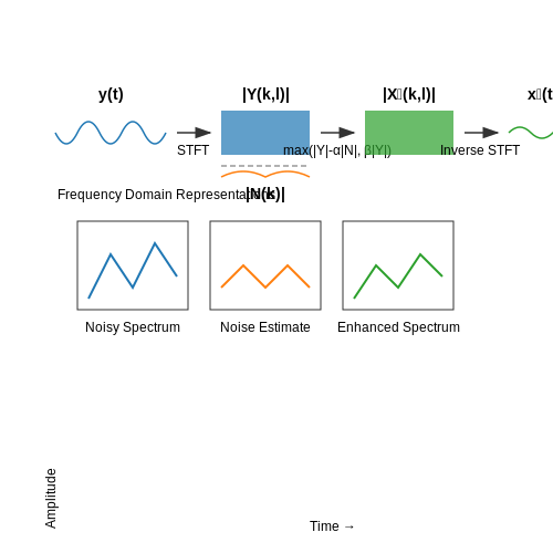
Spectral subtraction operates in the frequency domain to remove noise by estimating the noise spectrum and subtracting it from the noisy signal. Given a noisy signal y(t) composed of clean speech x(t) and additive noise n(t), the short-time Fourier transform (STFT) representation is:
where k denotes the frequency bin and l the time frame. The noise spectrum |N(k, l)| is estimated during non-speech intervals, typically using a voice activity detector (VAD). The enhanced signal magnitude spectrum is computed as:
Here, α is an over-subtraction factor (typically 1-2) and β is a spectral floor parameter (0.01-0.1) to prevent musical noise artifacts. The phase of Y(k, l) is retained for reconstruction via inverse STFT.
Wiener Filtering
The Wiener filter minimizes the mean square error between the estimated and true clean signal. In the frequency domain, the Wiener filter H(k) is given by:
where Pxx(k) and Pnn(k) are the power spectral densities of speech and noise, respectively. Practical implementations often use decision-directed estimation for Pxx(k):
with γ typically set to 0.98. This approach provides robust noise reduction while preserving speech components.
Non-Negative Matrix Factorization (NMF)
NMF decomposes the spectrogram V into basis W and activation H matrices under non-negativity constraints:
The optimization minimizes the Kullback-Leibler divergence:
For noise reduction, separate NMF models are trained for speech and noise. During enhancement, the speech components are reconstructed using only the speech basis vectors while suppressing noise contributions.
Deep Learning Approaches
Recent advances employ deep neural networks (DNNs) for end-to-end noise suppression. A typical architecture includes:
- Time-domain networks: WaveNet or Conv-TasNet variants operating directly on raw waveforms
- Time-frequency networks: U-Net or Transformer architectures processing spectrograms
- Hybrid approaches: Combining time and frequency domain processing
The loss function often combines spectral and waveform terms:
where α, β, γ are weighting factors and Ladv denotes adversarial loss for perceptual quality improvement.
Real-World Implementation Considerations
Practical systems must address:
- Latency constraints: Frame sizes below 20ms for real-time applications
- Computational complexity: Trade-offs between enhancement quality and processing resources
- Non-stationary noise: Adaptive noise estimation techniques
- Artifact suppression: Techniques to minimize musical noise and speech distortion
Modern implementations often combine traditional signal processing with machine learning, using DNNs for noise estimation while retaining Wiener filtering or spectral subtraction for actual suppression.
2.3 Segmentation and Speaker Diarization
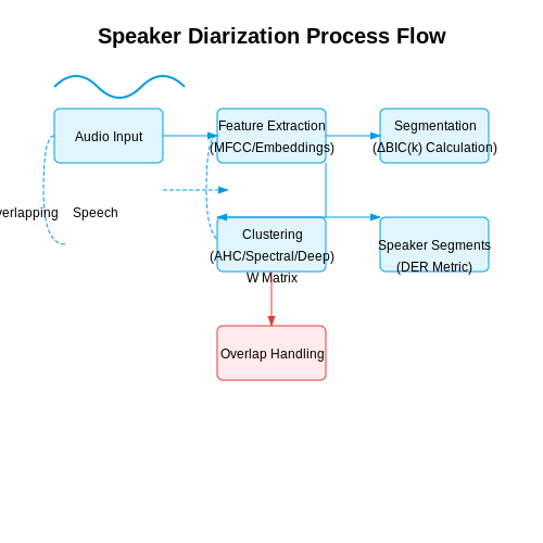
Speaker diarization is the process of partitioning an audio stream into homogeneous segments corresponding to individual speakers, answering the question "who spoke when?" without prior knowledge of speaker identities. This involves two key sub-tasks: speaker segmentation (detecting speaker change points) and speaker clustering (grouping segments by speaker identity).
Feature Extraction for Diarization
Modern diarization systems rely on spectral representations that capture speaker-discriminative characteristics. Mel-frequency cepstral coefficients (MFCCs) remain widely used, but recent approaches leverage deep neural network embeddings:
where y represents raw audio samples and xt is a fixed-dimensional embedding vector at time t with context window τ. State-of-the-art systems use architectures like:
- TDNN (Time-Delay Neural Networks) with statistical pooling
- ResNet variants operating on spectrograms
- Transformer-based models with self-attention
Speaker Change Detection
Bayesian Information Criterion (BIC) provides a mathematically rigorous approach for detecting speaker transitions. For a candidate segmentation point at frame k, the BIC difference is computed as:
where Σ represents covariance matrices of features before/after the candidate point, N is the number of frames, and P is the penalty term with dimensionality d:
Clustering Algorithms
After segmentation, speaker embeddings are clustered using:
- Agglomerative Hierarchical Clustering (AHC): Iteratively merges closest clusters until stopping criterion (threshold or number of speakers)
- Spectral Clustering: Forms affinity matrix W where Wij = exp(-γ||xi-xj||2), then performs eigenvalue decomposition
- Deep Embedded Clustering: Jointly optimizes neural network parameters and cluster assignments
Practical Considerations
Real-world diarization must handle overlapping speech, which requires:
- Independent voice activity detection (VAD) before diarization
- Multi-microphone arrays for spatial separation
- End-to-end neural approaches like Target-Speaker Voice Activity Detection (TS-VAD)
Current state-of-the-art systems achieve ~5% diarization error rate (DER) on clean speech, but performance degrades significantly with background noise and short speaker turns (<1s). Recent advances in self-supervised learning (e.g., wav2vec 2.0) show promise for improving robustness.
3. Automated Transcription of Call Recordings
Automated Transcription of Call Recordings
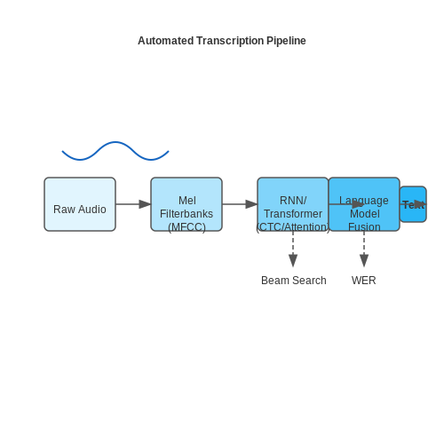
Automated transcription of call center audio relies on speech-to-text (STT) systems that convert spoken language into written text. Modern STT pipelines leverage deep learning architectures, primarily recurrent neural networks (RNNs) or transformer-based models like Whisper, which achieve state-of-the-art accuracy by jointly modeling acoustic and linguistic features.
Acoustic Feature Extraction
The first stage involves converting raw audio signals into a compact, discriminative representation. Mel-frequency cepstral coefficients (MFCCs) are commonly used, derived through the following steps:
where \( x[n] \) is the discrete-time signal, \( N \) is the frame length, and \( k \) corresponds to the frequency bin. The power spectrum is then warped to the Mel scale to approximate human auditory perception:
Recent systems replace handcrafted features with learnable filterbanks, allowing convolutional layers to adaptively extract task-relevant spectral patterns.
Sequence Modeling Architectures
Connectionist Temporal Classification (CTC) provides an alignment-free training objective for RNN-based transcribers:
where \( \pi \) is a path through the network's output distribution \( y \). The CTC loss marginalizes over all valid alignments between input frames and output tokens. Transformer models instead employ self-attention mechanisms:
This allows direct modeling of long-range dependencies in speech signals, outperforming RNNs on conversational speech with complex turn-taking patterns.
Language Model Integration
End-to-end systems often incorporate external language models through shallow fusion during beam search decoding:
where \( \lambda \) controls the relative weight of the acoustic model (AM) and language model (LM) scores. Recent work explores deep fusion approaches where the LM is integrated into the AM's hidden layers.
Domain Adaptation Challenges
Call center audio presents unique challenges including:
- Overlapping speech from multiple speakers
- Background noise from call center environments
- Domain-specific vocabulary (product names, procedures)
Effective solutions include:
- Data augmentation with simulated noise and reverberation
- Transfer learning from general speech corpora to call center data
- Active learning to prioritize difficult samples for human review
Speaker diarization systems based on spectral clustering or neural embeddings can separate mixed audio streams before transcription:
where \( \mathbf{e} \) represents speaker embedding vectors.
Performance Evaluation Metrics
Word Error Rate (WER) remains the standard benchmark, computed as:
where \( S \), \( D \), and \( I \) are substitutions, deletions, and insertions respectively, and \( N \) is the total reference words. Advanced systems achieve WERs below 5% on clean call center audio, though performance degrades significantly with poor recording quality or strong accents.
3.2 Sentiment Analysis and Emotion Detection
Sentiment analysis and emotion detection in call center audio involve extracting affective states from speech signals, leveraging both linguistic and paralinguistic features. Traditional sentiment analysis classifies utterances into positive, negative, or neutral categories, while emotion detection identifies finer-grained states such as anger, happiness, or frustration.
Feature Extraction for Affective Computing
Effective sentiment and emotion recognition rely on multimodal feature extraction:
- Prosodic features: Pitch (F0), energy, speaking rate, and pauses.
- Spectral features: Mel-frequency cepstral coefficients (MFCCs), formants, and spectral flux.
- Voice quality features: Jitter, shimmer, and harmonic-to-noise ratio (HNR).
- Lexical features: Word embeddings (e.g., BERT, GloVe) and sentiment lexicons.
The combined feature vector x for an audio segment can be represented as:
Machine Learning Architectures
Modern approaches employ hybrid architectures:
1. Temporal Modeling with RNNs
Long Short-Term Memory (LSTM) networks capture sequential dependencies in speech:
where ht is the hidden state at time t, and W matrices are learned weights.
2. Attention Mechanisms
Self-attention layers weight important temporal regions:
3. Multitask Learning
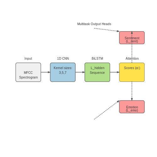
Jointly optimizing sentiment and emotion tasks improves performance:
Evaluation Metrics
Performance is measured using:
- Weighted F1-score: Accounts for class imbalance in call center data.
- Concordance Correlation Coefficient (CCC): Measures emotion intensity prediction.
- Unweighted Average Recall (UAR): Balanced accuracy across classes.
Practical Challenges
Real-world deployment faces several hurdles:
- Background noise: Call center environments often contain chatter and keyboard sounds.
- Code-switching: Agents and customers may mix languages.
- Cultural differences: Emotion expression varies across demographics.
Recent work addresses these through data augmentation and adversarial training. For example, SpecAugment applies time warping and frequency masking to audio spectrograms:
Case Study: Real-Time Emotion Detection
A deployed system for a European call center achieved 72% UAR using:
- 1D CNN for local feature extraction
- BiLSTM with attention for temporal modeling
- Knowledge distillation to reduce latency
The model processes audio in 500ms windows with 83ms stride, enabling real-time feedback to supervisors.
3.3 Topic Modeling and Keyword Extraction
Topic modeling and keyword extraction are essential techniques for uncovering latent themes and salient terms in call center audio transcripts. These methods transform unstructured conversational data into structured insights, enabling automated categorization and trend analysis.
Latent Dirichlet Allocation (LDA) for Topic Modeling
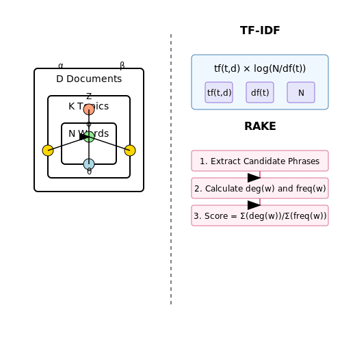
LDA is a generative probabilistic model that assumes documents are mixtures of topics, where each topic is a distribution over words. Given a corpus of D documents with N words each, LDA models the document-topic and topic-word distributions as Dirichlet processes:
where θd is the topic distribution for document d, ϕk is the word distribution for topic k, and Zd,n is the topic assignment for the n-th word in document d. The hyperparameters α and β control the sparsity of these distributions.
For call center applications, LDA can reveal recurring customer concerns (e.g., billing issues, technical support) without predefined labels. The model's output includes:
- Topic-word distributions showing key terms per theme
- Document-topic distributions for call categorization
- Topic coherence scores to evaluate semantic meaningfulness
Keyword Extraction Techniques
Beyond topic modeling, keyword extraction identifies the most salient terms in individual calls or call segments. Advanced methods include:
1. TF-IDF Weighting
Term Frequency-Inverse Document Frequency (TF-IDF) quantifies word importance by combining:
where tf(t,d) is term frequency in document d, N is total documents, and df(t) is document frequency of term t. High TF-IDF scores indicate call-specific keywords.
2. RAKE (Rapid Automatic Keyword Extraction)
RAKE identifies keywords by:
- Splitting text into candidate phrases at stopwords
- Scoring phrases by summing individual word scores
- Word scores based on degree (co-occurrences) and frequency
The final keyword score for a phrase is:
3. BERT-based Keyword Extraction
Transformer models like BERT capture contextual word importance through attention mechanisms. The process involves:
- Fine-tuning BERT on domain-specific call transcripts
- Extracting attention weights between [CLS] token and words
- Aggregating attention across layers to identify salient terms
Implementation Considerations
When applying these techniques to call center audio:
- Preprocessing: Remove filler words (e.g., "um", "ah") but retain negation terms
- Domain adaptation: Augment standard stopword lists with call-center specific terms
- Evaluation: Use human-annotated test sets to measure precision@k for keyword extraction
- Real-time processing: Implement incremental LDA for streaming call analysis
Practical applications include automated call routing based on detected topics, identifying emerging customer issues from keyword trends, and quality assurance through topic-based call monitoring.
4. Identifying Customer Pain Points and Trends
4.1 Identifying Customer Pain Points and Trends
Speech-to-Text Transcription and Semantic Parsing
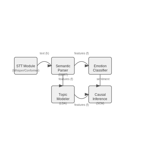
Accurate identification of customer pain points begins with high-fidelity speech-to-text (STT) transcription. Modern STT systems employ transformer-based architectures like Whisper or Conformer, achieving word error rates (WER) below 5% in clean audio conditions. The transcription output X is a sequence of words w1, w2, ..., wn, which is then parsed into structured semantic units using dependency parsing and named entity recognition (NER).
where hi-1 is the hidden state of the transformer at position i-1, and ewi is the embedding of word wi.
Sentiment and Emotion Analysis
Beyond lexical content, prosodic features (pitch, intensity, speech rate) are extracted using signal processing techniques like Praat or OpenSMILE. A multimodal emotion classifier combines:
- Lexical sentiment (BERT-based classifiers)
- Acoustic features (e.g., MFCCs, pitch contours)
- Conversational dynamics (turn-taking patterns, silence duration)
The combined feature vector f is fed into a hierarchical attention network:
Topic Modeling and Trend Extraction
Latent Dirichlet Allocation (LDA) with dynamic topic modeling tracks evolving pain points over time. For a corpus of D calls with vocabulary size V, the generative process is:
- For each topic k, draw word distribution βk ∼ Dir(η)
- For each call d at time t:
- Draw topic proportions θd ∼ Dir(α)
- For each word n:
- Draw topic assignment zdn ∼ Mult(θd)
- Draw word wdn ∼ Mult(βzdn)
Real-World Implementation Considerations
In production systems, streaming LDA variants handle call volume exceeding 10,000 calls/hour. Key optimizations include:
- Minibatch variational inference with GPU acceleration
- Incremental model updates via stochastic variational inference
- Dynamic thresholding for emerging topic detection
Root Cause Analysis with Causal Inference
Structural causal models (SCMs) disentangle correlation from causation in customer complaints. For variables X (e.g., product issue), Y (customer sentiment), and confounders Z, the causal effect is estimated via backdoor adjustment:
Instrumental variable methods handle unmeasured confounding when analyzing policy changes (e.g., new return policy effects on complaint frequency).
4.2 Agent Performance Evaluation and Coaching
Speech Analytics for Performance Metrics
Modern call center analytics employ deep neural networks to extract quantitative performance metrics from agent-customer interactions. The key metrics include:
- First Call Resolution (FCR): Derived from semantic analysis of call transcripts and subsequent interactions
- Average Handling Time (AHT): Computed through speech activity detection and turn-taking analysis
- Sentiment Trajectory: Time-dependent emotional state modeling using prosodic features and lexical analysis
where Ni represents total calls handled by agent i, and Resolvedj is a binary indicator function for successful resolution.
Conversation Quality Scoring
A hierarchical attention network processes multiple modalities to generate quality scores:
The weights (α, β, γ) are learned through backpropagation across thousands of labeled calls. The lexical component analyzes:
- Topic adherence through BERT-based embeddings
- Question density per minute
- Negative phrase avoidance
Real-time Coaching Systems
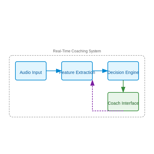
Edge computing enables low-latency feedback during live calls. The system architecture comprises:
The decision engine employs reinforcement learning to optimize intervention timing, balancing between:
- Immediate correction value
- Conversation flow disruption cost
- Agent cognitive load
Adaptive Threshold Policy
The system dynamically adjusts coaching triggers based on agent skill progression:
where λ represents the agent's learning rate, estimated through exponential decay modeling of historical performance metrics.
Multimodal Performance Benchmarking
Agent ranking incorporates both acoustic and linguistic dimensions through tensor factorization:
where A, B, and C represent factor matrices for agents, performance dimensions, and temporal segments respectively. The core tensor G captures nonlinear interactions between these modes.
4.3 Predictive Analytics for Call Outcomes
Feature Engineering for Call Outcome Prediction
Predictive modeling of call outcomes requires extracting discriminative features from both acoustic and linguistic dimensions. Key feature categories include:
- Prosodic features: Pitch contours (F0), speaking rate, intensity dynamics, and pause patterns
- Spectral features: MFCCs, spectral centroid, and harmonic-to-noise ratio
- Lexical features: Term frequency-inverse document frequency (TF-IDF) of transcribed text
- Dialog act features: Sequence of speech acts (questions, statements, confirmations)
- Temporal features: Response latency and turn-taking patterns
where ΔF0 quantifies pitch variability across T frames, a strong indicator of emotional state.
Architectures for Sequential Prediction
Call center interactions constitute temporal sequences where outcome probabilities evolve dynamically. The conditional probability of outcome y given features x1:t up to time t can be modeled as:
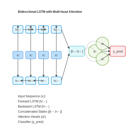
where ht is the hidden state of a bidirectional LSTM:
Attention Mechanisms for Interpretability
Multi-head attention weights αi,j reveal which dialog segments most influence predictions:
where qi, kj are learned query and key vectors of dimension d.
Evaluation Metrics for Imbalanced Data
Call outcomes often follow skewed distributions (e.g., rare escalations). The Fβ score provides better assessment than accuracy:
with β > 1 emphasizing recall for critical outcomes like customer churn.
Implementation Example: PyTorch Model
class CallOutcomePredictor(nn.Module):
    def __init__(self, input_dim, hidden_dim, num_classes):
        super().__init__()
        self.encoder = nn.LSTM(input_dim, hidden_dim, bidirectional=True)
        self.attention = nn.MultiheadAttention(hidden_dim*2, num_heads=4)
        self.classifier = nn.Linear(hidden_dim*2, num_classes)

    def forward(self, x):
        x, _ = self.encoder(x)  # (seq_len, batch, hidden_dim*2)
        attn_out, _ = self.attention(x, x, x)
        return self.classifier(attn_out.mean(dim=0))
Real-World Deployment Challenges
Production systems must handle:
- Concept drift: Customer behavior shifts over time requiring online learning
- Latency constraints: Real-time predictions during live calls
- Explainability: Regulatory requirements for decision justification
5. Compliance with Data Protection Regulations
5.1 Compliance with Data Protection Regulations
Processing call center audio data necessitates strict adherence to data protection laws such as the General Data Protection Regulation (GDPR), California Consumer Privacy Act (CCPA), and Health Insurance Portability and Accountability Act (HIPAA) where applicable. These regulations impose legal constraints on data collection, storage, processing, and sharing, particularly for personally identifiable information (PII) and sensitive personal data.
Key Regulatory Requirements
Under GDPR, audio recordings qualify as personal data if they can identify an individual. Key obligations include:
- Lawful Basis for Processing: Requires explicit consent or legitimate interest justification under Article 6(1)(f). For special category data (e.g., health information), additional conditions under Article 9 must be met.
- Data Minimization: Only collect audio data necessary for the specified purpose.
- Storage Limitation: Retain recordings only as long as required by the purpose or legal mandate.
- Right to Erasure: Individuals may request deletion of their data under Article 17.
Technical Implementation Challenges
Real-time audio analysis systems must embed privacy-preserving techniques:
Where identifiable features include speaker voiceprints, names, account numbers, or other PII. A score ≥0.9 is typically required for compliance. Practical implementations use:
- Automatic Speech Recognition (ASR) with Redaction: Replace PII tokens with placeholders during transcription.
- Voice Anonymization: Modify pitch, timbre, or formants using generative adversarial networks (GANs) while preserving linguistic content.
- Differential Privacy: Add controlled noise to acoustic features during analysis to prevent re-identification.
Architectural Considerations
A compliant pipeline requires:
The access control layer enforces role-based permissions and audit logging per ISO/IEC 27001 standards. Encryption must be applied both in transit (TLS 1.3+) and at rest (AES-256 with proper key management).
Cross-Border Data Transfers
When processing spans multiple jurisdictions, mechanisms like GDPR Standard Contractual Clauses (SCCs) or binding corporate rules (BCRs) must be implemented. For US-EU transfers, the Data Privacy Framework (DPF) adequacy decision provides a compliance pathway.
5.2 Anonymization and Secure Handling of Audio Data
Audio Data Anonymization Techniques
Anonymizing call center audio requires removing or obfuscating personally identifiable information (PII) while preserving linguistic content for analysis. The most effective methods include:
- Voice De-identification: Applying voice conversion techniques to modify speaker characteristics while maintaining linguistic content. This can be achieved through:
where \(X\) is the original speech signal, \(s_{target}\) is a target speaker embedding, and \(f_\theta\) is a neural voice conversion model.
- Selective Audio Redaction: Using automatic speech recognition (ASR) combined with named entity recognition (NER) to detect and mute PII segments.
- Prosody Preservation: Maintaining emotional content while removing identity markers through spectral feature manipulation.
Secure Storage Architectures
For compliance with GDPR and other regulations, audio data must be stored using:
- End-to-end encryption: AES-256 encryption for data at rest combined with TLS 1.3 for data in transit.
- Tokenization systems: Where raw audio is stored encrypted while analysis systems work with tokenized representations.
- Differential privacy: Adding controlled noise to acoustic features during analysis:
where \(\sigma\) is calibrated to the privacy budget \(\epsilon\).
Access Control Mechanisms
Implementing zero-trust architectures requires:
- Role-based access control (RBAC) with attribute-based encryption
- Multi-party computation for sensitive operations
- Blockchain-based audit trails for all data accesses
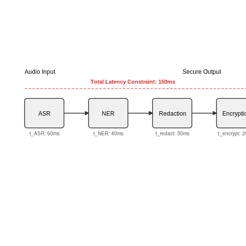
Real-time Processing Constraints
Secure real-time processing introduces latency constraints. The end-to-end delay \(D\) must satisfy:
This requires optimized pipelines using:
- Quantized neural networks for ASR/NER
- Hardware-accelerated encryption (Intel SGX, AWS Nitro)
- Edge computing for initial processing
Compliance Verification
Automated compliance checking involves:
- Adversarial re-identification tests to validate anonymization
- Formal verification of encryption implementations
- Regular penetration testing of storage systems
5.3 Bias and Fairness in Audio Analysis
Audio analysis models, particularly those deployed in call centers, are susceptible to biases that can propagate unfair outcomes. These biases often stem from imbalanced training data, algorithmic design choices, or the embedding of sociocultural prejudices into model predictions. Understanding and mitigating these biases is critical for ensuring equitable treatment across diverse speaker demographics.
Sources of Bias in Audio Analysis
Bias in audio analysis can originate from multiple stages of the machine learning pipeline:
- Data Collection Bias: Training datasets often underrepresent minority dialects, non-native speakers, or regional accents. For example, a model trained predominantly on North American English may perform poorly on Indian English or African American Vernacular English (AAVE).
- Feature Extraction Bias: Acoustic features like pitch, formants, or speech rate can correlate with gender or age, leading to skewed predictions. Mel-frequency cepstral coefficients (MFCCs) may encode sociolinguistic variations that are irrelevant to the task.
- Labeling Bias: Human annotators may unconsciously associate certain speech patterns with negative sentiment or lower competence, especially when dealing with non-standard dialects.
Quantifying Bias Mathematically
To measure bias, we can define disparity metrics across protected attributes (e.g., gender, race, age). Let Ŷ be the model's predictions and S be a sensitive attribute with k classes. The demographic parity difference (DPD) is:
For continuous outcomes like sentiment scores, we can compute the Wasserstein distance between score distributions across groups:
where Γ(Pi, Pj) is the set of all joint distributions with marginals Pi and Pj.
Mitigation Strategies
Pre-processing Techniques
Adversarial debiasing modifies the feature space to remove sensitive information while preserving predictive power. The objective is:
where fθ is the main model, and the adversary φ tries to predict S from the features.
In-processing Methods
Fairness constraints can be directly incorporated into the optimization. For a logistic regression model with weights w, we might add a covariance constraint:
This ensures the predictions are minimally correlated with the sensitive attribute.
Post-hoc Calibration
Group-specific thresholds can be tuned to equalize performance metrics. For a binary classifier, we solve:
where Ŷτ is the thresholded prediction.
Case Study: Accent Bias in Emotion Recognition
A 2022 study found that commercial emotion recognition systems showed 15-20% lower accuracy for speakers with Southern U.S. accents compared to General American accents when detecting anger. The bias was traced to:
- Underrepresentation of Southern accents in training data (only 8% of samples)
- Higher false positive rates for anger due to stereotypical associations with Southern speech patterns
After applying adversarial debiasing and oversampling underrepresented accents, the accuracy gap reduced to 3-5% while maintaining overall model performance.
Implementation Considerations
When deploying fairness-aware models in call centers:
- Monitor performance disparities across customer segments in real-time using A/B testing frameworks
- Implement fallback mechanisms when confidence scores differ significantly across demographics
- Regularly audit models using techniques like SHAP (SHapley Additive Explanations) to detect emergent biases
6. Key Research Papers and Articles
6.1 Key Research Papers and Articles
- Telephone Call Centers: Tutorial, Review, and Research Prospects — stitutions Center (N.G. and A.M.), The Wharton Electronic Business Initiative (N.G.), Israeli Science Foundation (ISF) Grants 388/99 and 126/02 (A.M.), and the Technion funds for the promotion of research and sponsored research (A.M.). Some data originated with member companies of the Call Center Forum at Wharton, to whom we are grateful.
- Multimodal evaluation of customer satisfaction from voicemails using ... — This research proposes a methodology for analyzing CS in call-center voicemails by integrating speech and language modalities. This study aims to explore different fusion techniques to improve the evaluation process and provide valuable insights to call-center managers. ... and comprises audio recordings from a call-center. This corpus allows ...
- PDF Analyzing VoIP connectivity and performance issues - DiVA — jitter [2], these factors affect directly the call quality and can result in choppy voice, echoes, or even in a call failure. The main objective of this work was to create a tool for automatic analysis and evaluation from packet traces, identify connectivity and performance issues, reconstruct the audio streams and estimate the call quality.
- Development of Speech Recognition Systems in Emergency Call Centers - MDPI — In this paper, various methodologies of acoustic and language models, as well as labeling methods for automatic speech recognition for spoken dialogues in emergency call centers were investigated and comparatively analyzed. Because of the fact that dialogue speech in call centers has specific context and noisy, emotional environments, available speech recognition systems show poor performance.
- Noise Exposure and Hearing Status Among Employees Using Communication ... — For example earlier, Patel and Brougthon visited 15 call centers in the United Kingdom in order to evaluate whether or not there was a risk to hearing from working in a call center. They measured noise exposure in 150 operators and revealed that the corrected noise levels generated by headsets fitted on the KEMAR manikin ranged 65-88 dB ...
- PDF arXiv:2203.06396v1 [cs.CL] 12 Mar 2022 — center domain, where speech analytics is an extremely powerful methodology for gaining insights from unstructured data, coming from customer and human agent conversations. In this work, we describe an experimentation with a speech analytics process for an Italian contact center, that deals with call recordings extracted from inbound or outbound ...
- Formulation of an AI-Based Call Analytics Model for ... - Springer — In this research, audio from inbound calls will be converted to text, and AI will auto-classify mixed-language texts into topics, intentions, sentiment analysis, and emotions. ... The result is a text file that contains the exchange between the agent and the customer in a call center. However, this study highlights the challenges after ...
- (PDF) Voice‐based AI in call center customer service ... - ResearchGate — call center customer service setting and offers usefu l insights into how AI-powered service flexibility impacts different outcom es in human-AI interactions (Luo et al. 2019, Sun et a l. 2019 ...
- An Introduction to Audio Content Analysis - Wiley Online Library — Audio content analysis, a subfield of the research field music infor-mation retrieval, aims at extracting (musical and perceptual) properties directly from the audio signal to support these tasks. Knowledge of these properties allows us to improve the interaction of humans or machines with digital audio signals. It enables new ways of
- (PDF) The Modern Call Center: A Multi‐Disciplinary ... - ResearchGate — Call centers are an increasingly important part of today's business world, employing millions of agents across the globe and serving as a primary customer‐facing channel for firms in many ...
6.2 Recommended Tools and Libraries
- An introduction to audio content analysis [electronic resource ... — Stanford Libraries' official online search tool for books, media ... An introduction to audio content analysis [electronic resource] : applications in signal processing and music informatics ... 202 D.1.1 Marsyas 202 D.1.2 CLAM 202 D.1.3 jMIR 203 D.1.4 CoMIRVA 203 D.1.5 Sonic Visualiser 203 D.2 Software Libraries & Toolboxes 204 D.2.1 Feature ...
- An Introduction to Audio Content Analysis - Wiley Online Library — electronic, mechanical, photocopying, recording, scanning, or otherwise, except as permitted under Section 107 or 108 of ... D Software for Audio Analysis 201 D. 1 Software Frameworks and Applications 202 D.l.l Marsyas 202 D.1.2 CLAM 202 D.I.3 jMIR 203 D.I.4 CoMIRVA 203 D.1.5 Sonic Visualiser 203 D.2 Software Libraries and Toolboxes 204 D.2.1 ...
- Cisco Nexus Dashboard Insights — Collections. Licensing; Nexus Dashboard Licensing Information ; Release; Cisco Nexus Dashboard Insights, Release 6.5.1 User Content for NDFC or Standalone NX-OS ; Cisco Nexus Dashboard Insights, Release 6.5.1 User Content for ACI ; Cisco Nexus Dashboard Insights, Release 6.4.1 User Content for NDFC or Standalone NX-OS ; Cisco Nexus Dashboard Insights, Release 6.4.1 User Content for ACI
- PDF arXiv:2203.06396v1 [cs.CL] 12 Mar 2022 — center domain, where speech analytics is an extremely powerful methodology for gaining insights from unstructured data, coming from customer and human agent conversations. In this work, we describe an experimentation with a speech analytics process for an Italian contact center, that deals with call recordings extracted from inbound or outbound ...
- Audiogmenter: a MATLAB toolbox for audio data augmentation — To the best of our knowledge, Audiogmenter is the first MATLAB library specifically designed for audio data augmentation. Such libraries exist in other languages like Python. A well-known Python audio library is Librosa . The aim of Librosa was to create a set of tools to mine audio databases, but the result was an even more comprehensive ...
- PDF Oracle Call Center Intelligence — 1.1 What is Oracle Call Center Intelligence? Oracle Call Center Intelligence (ICI) is an Internet-ready performance-management application for Oracle Interaction Center applications. By merging interaction data with business data, the application can provide unique insight into the interaction center's operations and business results.
- Unlocking Business Insights from Audio with AWS Transcribe, Comprehend ... — generation of subtitles on audio and video content; conversion of audio file (for example podcast) to text; search for keywords or inappropriate words within an audio file . AWS Transcribe. At the re:invent2017 conference, Amazon Web Services presented Amazon Transcribe, a new, machine learning - natural language processing - service.
- Azure Application Insights libraries for .NET - Azure for .NET ... — The Application Insights client SDK for .NET allows you to log event, aggregated data, exceptions, dependency, and metrics to Azure for future analysis. Install the NuGet package directly from the Visual Studio Package Manager console or with the .NET Core CLI. Visual Studio Package Manager Install-Package Microsoft.ApplicationInsights
- (PDF) Voice‐based AI in call center customer service ... - ResearchGate — call center customer service setting and offers usefu l insights into how AI-powered service flexibility impacts different outcom es in human-AI interactions (Luo et al. 2019, Sun et a l. 2019 ...
- Introduction to Audio Analysis - O'Reilly Media — Book description. Introduction to Audio Analysis serves as a standalone introduction to audio analysis, providing theoretical background to many state-of-the-art techniques. It covers the essential theory necessary to develop audio engineering applications, but also uses programming techniques, notably MATLAB®, to take a more applied approach to the topic.
6.3 Industry Case Studies and Reports
- Call Center Analytics: What They are and How to Use Them ... - AmplifAI — Uses AI to analyze call recordings for insights on words, audio patterns, emotions, and performance. 2: Text Analytics: Analyzes written communications to extract insights and improve call center operations. 3: Predictive Analytics: Forecasts future trends and outcomes using historical data to enhance operational efficiency. 4: Interaction ...
- Contact Center Analytics Market Size, Industry Share Forecast — 2.1.2.2 Key industry insights 2.2 MARKET BREAKUP AND DATA TRIANGULATION ... FIGURE 19 EVOLUTION OF CONTACT CENTER ANALYTICS 5.5 CASE STUDY ANALYSIS 5.5.1 BANKING, FINANCIAL SERVICES, AND INSURANCE ... 11.6.3.1 Businesses using contact center solutions to connect with customers 11.6.4 REST OF LATIN AMERICA. 12 COMPETITIVE LANDSCAPE (Page No ...
- Contact Center Analytics Market Share, Size and Industry Growth ... — Contact Center Analytics Market Overview. Contact Center Analytics Market size is analyzed to grow at a CAGR of 18.8% during the forecast 2022-2027 to reach $$930.4 million by 2027. Call Center analytics is the process of gathering and analyzing customer data in order to gain important insights into the functioning of a service company.
- Contact Center Analytics Market Size, Share & Growth, 2034 — Contact Center Analytics Market | Global Industry Report, Size, Share, Growth, Price Analysis, Trends, Outlook and Forecast 2025-2034 The global contact center analytics market hit USD 1.80 Billion in 2024 and is expected to grow at a 19.60% CAGR, reaching USD 10.78 Billion by 2034.
- Global Call Center Analytics Market Research Report 2023 — According to QYResearch's new survey, global Call Center Analytics market is projected to reach US$$ 2265.2 million in 2029, increasing from US$ 956 million in 2022, with the CAGR of 13.6% during the period of 2023 to 2029.
- Call Center AI Market Size, Share, Trends Report | Growth - 2031 — 10.6.1 rising need to automate contact center processes and gain customer insights to boost call center ai growth table 77 sentiment analysis: market, by region, 2016-2021 (usd million) table 78 sentiment analysis: market, by region, 2022-2027 (usd million) 10.7 appointment scheduling
- Contact Center Software Market - Size, Companies & Growth — Contact Center Software Market Analysis. The Contact Center Software Market size is estimated at USD 72.62 billion in 2025, and is expected to reach USD 172.64 billion by 2030, at a CAGR of 18.91% during the forecast period (2025-2030). The market is primarily driven by the increasing need to enhance customer experience at relatively lower costs.
- Making a case for speech analytics to improve customer service quality ... — In this case study, we present a strategic initiative that examines the use of speech analytics to improve customer service quality at call centers, or contact centers, of a company in the U.S. healthcare industry, Crossroads WellNet (pseudonym).This is a worthwhile endeavor at Crossroads WellNet because it attempts to determine whether or not speech analytics tools can be effective in ...
- Contact Center Analytics Market - Future Market Insights — Newly-released Contact Center Analytics Market analysis report by Future Market Insights shows that global sales of the Contact Center Analytics Market in 2021 were held at USD 1.2 Billion. With 16.2%, the projected market growth from 2022 to 2032 is expected to be slightly higher than the historical growth.
- (PDF) Automated transcription of conversational Call Center speech ... — We provide a case study on a real-life, large-scale data of more than 800K call transcripts from a large financial services company in the U.S. to examine the practical features and challenges of ...