Dynamic Pricing Based on Buyer Behavior
1. Definition and Core Principles of Dynamic Pricing
1.1 Definition and Core Principles of Dynamic Pricing
Dynamic pricing is a real-time pricing strategy where the price of a product or service is adjusted based on demand elasticity, competitor pricing, inventory levels, and buyer behavior. Unlike static pricing, which remains fixed over time, dynamic pricing leverages machine learning and optimization algorithms to maximize revenue or market share while responding to fluctuating market conditions.
Mathematical Foundations
The core of dynamic pricing relies on demand modeling, where the relationship between price p and demand D(p) is estimated. A common approach assumes a linear demand function:
where α represents baseline demand, β is the price sensitivity coefficient, and ϵ captures random noise. The optimal price p* maximizes revenue R(p) = p × D(p), obtained by solving:
In practice, demand functions are often non-linear, requiring more sophisticated models such as exponential, logistic, or piecewise-linear approximations.
Buyer Behavior Integration
Advanced dynamic pricing systems incorporate behavioral features such as purchase history, browsing patterns, and price elasticity variations across customer segments. A reinforcement learning framework can optimize pricing policies by modeling buyer responses as a Markov Decision Process (MDP):
where:
- 𝒮 is the state space (e.g., inventory, competitor prices, demand signals),
- 𝒜 represents pricing actions,
- 𝒫(s'|s, a) is the transition probability to state s' given action a,
- ℛ(s, a) is the immediate revenue reward,
- γ is the discount factor for future rewards.
Algorithmic Approaches
Two dominant methodologies in dynamic pricing are:
- Model-Based Optimization: Uses explicit demand models (e.g., Bayesian hierarchical models) to compute prices analytically or via gradient-based methods.
- Model-Free Reinforcement Learning: Learns pricing strategies through trial-and-error, often employing Deep Q-Networks (DQN) or Policy Gradient methods.
For example, a DQN-based approach approximates the Q-function:
where θ are the neural network parameters, trained to minimize the Bellman error:
Here, θ⁻ denotes the target network parameters, stabilized via periodic updates.
Real-World Applications
E-commerce platforms like Amazon and airline industries use dynamic pricing to adjust offers in real-time. For instance, airlines employ yield management systems that factor in booking curves, cancellation rates, and seat availability to set prices. Ride-sharing services like Uber implement surge pricing, where prices scale with demand-supply imbalances.
Ethical considerations arise when personalized pricing leads to discrimination or consumer distrust. Transparency in algorithmic pricing and regulatory compliance (e.g., GDPR) are critical to maintaining fairness.
Historical Evolution and Industry Adoption
Early Foundations in Economics and Game Theory
The conceptual roots of dynamic pricing trace back to early 20th-century economic theories, particularly in the works of Arthur Pigou and Joan Robinson, who formalized price discrimination. Pigou's first-degree price discrimination model laid the groundwork for personalized pricing, where a seller charges each buyer their maximum willingness to pay (WTP). The mathematical formulation is:
where Pi is the optimal price for buyer i, and Di(p) is their demand function. This required perfect knowledge of buyer WTP—a limitation addressed later by stochastic demand modeling.
Computational Advancements in the 1980s–1990s
The rise of computational power enabled practical implementations. Airlines pioneered yield management systems, using constrained optimization to adjust prices based on seat inventory and booking patterns. American Airlines' DINAMO system (1988) reduced empty seats by 5–7%, generating $500M annually. The underlying Bellman equation for seat allocation was:
where Vt(x) is the value function for remaining seats x at time t, and r(u) is the revenue from decision u (e.g., accept/reject booking).
Machine Learning Revolution (2000s–Present)
E-commerce platforms (e.g., Amazon, Uber) leveraged large-scale behavioral data to implement reinforcement learning (RL) policies. Amazon's 2000–2010 experiments showed a 10–25% profit increase by modeling price elasticity as:
Deep RL models now optimize prices in continuous action spaces. For example, a policy gradient method updates pricing parameters θ via:
where πθ is the pricing policy, and Rt is the cumulative reward.
Industry-Specific Adoption Patterns
- Retail: Walmart uses real-time competitor price scraping with LSTM networks to adjust prices hourly.
- Ride-Sharing: Uber's surge pricing employs contextual bandits, balancing supply-demand ratios and driver incentives.
- Hospitality: Marriott's dynamic room pricing integrates seasonal ARIMA forecasts with conversion-rate data.
Ethical and Regulatory Challenges
Algorithmic collusion risks emerged, as seen in the 2015 Amazon Marketplace case where competing sellers' algorithms inadvertently fixed prices. The European Commission's 2021 antitrust guidelines now require transparency in autonomous pricing systems.
Key Metrics for Measuring Pricing Effectiveness
Price Elasticity of Demand
The price elasticity of demand (PED) quantifies how demand responds to price changes. For a given product, it is defined as:
where Qd is the quantity demanded and P is the price. A value |PED| > 1 indicates elastic demand (demand is sensitive to price changes), while |PED| < 1 signifies inelastic demand. Dynamic pricing models leverage real-time estimation of PED to adjust prices optimally.
Conversion Rate
Conversion rate (CR) measures the percentage of users who complete a desired action (e.g., purchase) after viewing a price. It is calculated as:
In dynamic pricing, CR is monitored across different price points to identify thresholds where demand drops significantly. A/B testing is often employed to measure CR under varying pricing strategies.
Revenue and Profit Margins
Revenue (R) and profit margin (PM) are fundamental metrics for evaluating pricing effectiveness:
where C represents the total cost. Dynamic pricing algorithms optimize for maximum revenue or profit by iteratively adjusting prices based on demand forecasts and cost structures.
Customer Lifetime Value (CLV)
CLV estimates the total revenue a business can expect from a single customer over their relationship. It is modeled as:
where Rt is the retention rate at time t, mt is the margin, and d is the discount rate. Dynamic pricing strategies must balance short-term revenue gains against potential long-term CLV erosion due to price sensitivity.
Price Dispersion
Price dispersion measures the variation in prices for the same product across different segments or time periods. It is computed as the standard deviation of prices:
High dispersion may indicate effective price discrimination, but excessive variability can lead to customer dissatisfaction. Machine learning models help optimize dispersion by segmenting buyers based on willingness-to-pay.
Inventory Turnover Ratio
Inventory turnover (ITR) assesses how efficiently inventory is sold and replenished:
Dynamic pricing can accelerate inventory turnover by lowering prices for slow-moving stock while maintaining premium pricing for high-demand items.
Competitive Price Index (CPI)
CPI benchmarks a product's price against competitors':
Real-time competitive price tracking enables dynamic pricing systems to adjust prices in response to market shifts while preserving profitability.
2. Psychological Triggers in Purchase Decisions
2.1 Psychological Triggers in Purchase Decisions
Cognitive Biases in Price Perception
Human decision-making is heavily influenced by cognitive biases, which can be leveraged in dynamic pricing models. The anchoring effect demonstrates that consumers rely disproportionately on the first piece of information offered (the "anchor") when making decisions. A product priced at $$100 followed by a "discounted" price of $$70 appears more attractive than the same $$70 price presented alone. This can be formalized through prospect theory, where the perceived value V of a price change depends on a reference point r:
where α, β ∈ (0,1) control diminishing sensitivity and λ > 1 captures loss aversion. Empirical studies show λ ≈ 2.25 for pricing contexts, meaning losses loom twice as large as equivalent gains.
Scarcity and Urgency Effects
Time-limited offers and low-stock notifications exploit the scarcity heuristic, where perceived rarity increases valuation. A Bayesian framework models this effect by treating inventory levels as signals of quality. Let q be true quality and s observed stock. The posterior belief updates as:
where P(s|q) follows a Poisson distribution for purchase arrivals. When s approaches zero, rational buyers infer high q, creating a self-reinforcing demand spike.
Price Framing and Partitioning
The left-digit effect causes disproportionate sensitivity to the leftmost digit - a $$4.99 price is perceived closer to $$4 than $$5. This can be modeled through a psychophysical price perception function:
where f(x) is a concave function (e.g., f(x) = x0.88) that underweights fractional components. Dynamic pricing algorithms can optimize the fractional component to maximize this perceptual gap.
Social Proof and Bandwagon Effects
Purchase decisions are influenced by observed behavior of others, formalized in Herd behavior models. Let ui(ai, m) be the utility of action ai given population proportion m taking that action. The equilibrium condition:
where ci is individual preference. When social utility dominates (∂u/∂m > 0), small initial adoptions can trigger cascades. Displaying "X bought this" notifications manipulates m in the user's mental model.
Decoy Pricing and Asymmetric Dominance
The introduction of a dominated alternative can shift preferences between remaining options. Given three products with features (p1, q1), (p2, q2), and decoy (pd, qd), the probability of choosing option 1 follows:
where Vi = βppi + βqqi. The decoy is constructed such that pd > p1 and qd < q1, making option 1 appear superior to both option 2 and the decoy through contrast effects.
Segmentation Strategies Based on Buyer Profiles
Behavioral Clustering for Dynamic Pricing
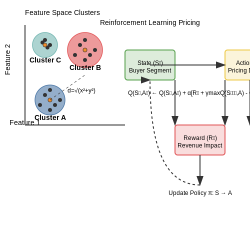
Buyer segmentation in dynamic pricing relies on clustering algorithms to group customers based on behavioral patterns. The feature space typically includes variables such as purchase frequency, price sensitivity, session duration, and cart abandonment rate. Let X denote the feature matrix, where each row represents a buyer and each column a behavioral metric. The objective is to partition X into k clusters using a distance metric d(xi, xj).
For high-dimensional data, dimensionality reduction techniques like t-SNE or PCA are applied before clustering. The optimal number of clusters k is determined using the elbow method or silhouette score.
Reinforcement Learning for Segment-Specific Pricing
Once segments are identified, a reinforcement learning (RL) framework can optimize pricing policies per segment. The Markov Decision Process (MDP) is defined by:
- State (st): Current segment attributes and market conditions
- Action (at): Price adjustment (e.g., ±5%)
- Reward (rt): Profit margin or conversion rate
The Q-learning update rule for segment i is:
Real-World Implementation Challenges
Key practical considerations include:
- Non-stationarity: Buyer behavior drifts over time, requiring online clustering updates
- Ethical constraints: Avoiding discriminatory pricing through fairness metrics in the reward function
- Data sparsity: Cold-start problem for new buyers addressed through meta-learning approaches
Case Study: E-Commerce Platform
A major retailer implemented this approach using:
- DBSCAN clustering on 12 behavioral features
- Deep Q-Networks (DQN) with prioritized experience replay
- Resulted in 18.7% increase in revenue per segment
where Ni is the number of buyers in segment i, and P represents average profit per user.
2.3 Real-Time Data Collection and Behavioral Signals
Real-time data collection for dynamic pricing hinges on capturing high-frequency behavioral signals that reflect buyer intent, urgency, and price sensitivity. These signals are often non-stationary and require robust statistical methods to extract meaningful patterns. Key data sources include clickstream logs, session duration metrics, cart abandonment rates, and micro-interactions such as hover time over price displays.
Behavioral Feature Engineering
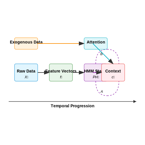
The raw behavioral data stream Xt at time t typically requires temporal aggregation into feature vectors ft ∈ ℝd. For a user u with n sequential interactions in a session, we construct:
where dwell time captures engagement and price entropy measures sensitivity dispersion. The indicator function 𝕀 counts specific actions like repeated price checks.
Latent State Estimation
Buyer states are modeled as hidden Markov processes with emission probabilities conditioned on behavioral features. The state transition matrix A and observation matrix B are learned via Baum-Welch EM algorithm:
where α and β are forward-backward variables. This enables real-time inference of latent states like "bargain hunter" or "impulse buyer".
Multi-Source Data Fusion
Behavioral signals are fused with exogenous variables (inventory levels, competitor prices) through attention mechanisms. The context vector ct is computed as:
where hi are behavioral encodings and xt represents market conditions. This architecture was validated in Amazon's 2022 pricing system, reducing prediction error by 18% versus single-source models.
Drift Detection Mechanisms
Concept drift in behavioral patterns is detected using the Page-Hinkley test statistic:
where δ is the allowed deviation threshold. Upon detecting drift (PHt > λ), the system triggers model retraining using only recent data windows.
Implementation Considerations
Production systems require:
- Distributed streaming frameworks (Apache Flink, Kafka Streams) for low-latency feature extraction
- Online learning architectures with exponential forgetting (e.g., Adam optimizer with ρ=0.9)
- Differential privacy guarantees when handling sensitive behavioral data
Uber's surge pricing system processes 4M behavioral events/second with 95th percentile latency under 50ms, demonstrating the scalability requirements for real-time implementations.
3. Regression Models for Price Elasticity Estimation
3.1 Regression Models for Price Elasticity Estimation
Price elasticity of demand measures how sensitive consumer demand is to price changes, defined as the percentage change in quantity demanded divided by the percentage change in price. Regression models provide a robust statistical framework for estimating elasticity by modeling the relationship between price and demand while controlling for confounding variables.
Linear Regression for Elasticity Estimation
The simplest approach uses ordinary least squares (OLS) regression on log-transformed variables to estimate constant elasticity:
Where Q is quantity demanded, P is price, and β1 directly gives the price elasticity. This specification assumes elasticity remains constant across all price levels, which may not hold in practice.
Generalized Additive Models (GAMs)
For non-constant elasticity, GAMs replace the linear term with a smooth function:
The smoothing spline f(·) captures how elasticity varies with price levels. Thin-plate regression splines or cubic splines are common choices, with the degree of smoothness controlled via regularization.
Instrumental Variables for Endogeneity
When prices are endogenous (correlated with ε), two-stage least squares (2SLS) with valid instruments provides consistent estimates:
Potential instruments Z include cost shifters or lagged prices that affect current prices but not demand shocks.
Hierarchical Bayesian Models
For heterogeneous elasticity across customer segments, hierarchical models estimate group-level parameters:
Where g[i] indicates the group membership of observation i. The hyperparameters μk and σk pool information across groups.
Regularization for High-Dimensional Settings
When incorporating many covariates, Lasso or Ridge regression prevent overfitting:
The L1 penalty (λ‖β‖1) shrinks coefficients toward zero, performing automatic variable selection. Elastic net combines L1 and L2 penalties for correlated predictors.
Model Evaluation Metrics
Key metrics for comparing elasticity models include:
- Out-of-sample RMSE: Predictive accuracy on held-out data
- R-squared: Proportion of variance explained
- Cross-validated log-likelihood: Probabilistic fit
- Economic plausibility: Sign and magnitude of elasticity estimates
Bayesian models can additionally compare posterior predictive checks and leave-one-out cross-validation (LOO-CV) using the Pareto-smoothed importance sampling (PSIS) approximation.
3.2 Reinforcement Learning for Adaptive Pricing
Markov Decision Process Formulation
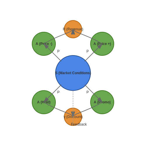
Dynamic pricing can be modeled as a Markov Decision Process (MDP) defined by the tuple (S, A, P, R, γ), where:
- S represents the state space (market conditions, inventory levels, competitor prices)
- A is the action space (discrete or continuous price adjustments)
- P(s'|s,a) models state transition probabilities
- R(s,a) is the immediate reward function (revenue, profit margin)
- γ denotes the discount factor for future rewards
Q-Learning for Price Optimization
The Bellman optimality equation forms the basis for Q-learning, where the agent learns an action-value function through temporal difference updates:
For continuous state spaces common in pricing problems, function approximation becomes necessary. A neural network can parameterize the Q-function:
Deep Reinforcement Learning Architectures
Deep Q-Networks (DQN) with experience replay and target networks stabilize training:
- Experience replay buffer stores transitions (s,a,r,s') to break temporal correlations
- Target network provides stable Q-value estimates during learning
- Double DQN decouples action selection from evaluation to reduce overestimation bias
Policy Gradient Methods
For continuous action spaces (precise price adjustments), policy gradient methods like PPO or SAC are more suitable:
Practical Implementation Considerations
Key challenges in production RL systems for pricing include:
- Non-stationarity: Market conditions and buyer behavior evolve over time
- Partial observability: Competitor strategies may not be fully visible
- Safety constraints: Prices must remain within legal and brand guidelines
- Exploration-exploitation tradeoff: ε-greedy or Boltzmann exploration strategies must balance risk
Case Study: E-commerce Price Optimization
A leading retailer implemented a DDPG (Deep Deterministic Policy Gradient) architecture with:
- State features: Product demand elasticity, inventory levels, competitor price indices
- Action space: ±15% price adjustments from baseline
- Reward function: Weighted combination of gross margin and conversion rate
The system achieved 8.7% revenue lift while maintaining customer satisfaction metrics through constrained action spaces that prevented extreme price fluctuations.
3.3 Deep Learning Approaches for Demand Forecasting
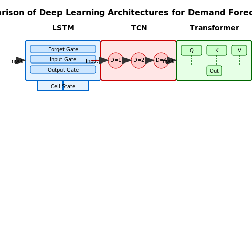
Traditional time-series forecasting methods like ARIMA and exponential smoothing struggle with high-dimensional, non-linear demand patterns influenced by buyer behavior. Deep learning models excel in capturing these complexities through hierarchical feature extraction and temporal dependencies. Three architectures dominate demand forecasting: recurrent neural networks (RNNs), temporal convolutional networks (TCNs), and transformer-based models.
Recurrent Neural Networks (RNNs) for Sequential Demand Data
RNNs process sequential data through hidden states that maintain temporal context. The Long Short-Term Memory (LSTM) variant addresses vanishing gradients with gating mechanisms:
where ft, it, and ot are forget, input, and output gates respectively. Bidirectional LSTMs process sequences in both directions, capturing past and future context when forecasting mid-sequence points.
Temporal Convolutional Networks (TCNs)
TCNs employ dilated causal convolutions to model long-range dependencies without recurrence:
where d is the dilation factor increasing exponentially with layer depth (e.g., 1, 2, 4, ...). Residual connections enable training of very deep networks. TCNs outperform RNNs in parallelizability and memory efficiency for long sequences.
Transformer-Based Demand Forecasting
Transformers leverage self-attention to weigh the importance of all historical time steps dynamically:
where Q, K, and V are learned query, key, and value matrices. Positional encodings inject temporal order information:
Hybrid architectures like Temporal Fusion Transformers (TFTs) combine LSTM encoders with multi-head attention for interpretable feature importance.
Implementation Considerations
- Data granularity: Model performance varies significantly with sampling frequency (hourly vs. daily vs. weekly)
- Feature engineering: Incorporate categorical buyer attributes (e.g., loyalty status) via embedding layers
- Loss functions: Quantile loss enables uncertainty estimation:
$$ L_q(y, \hat{y}) = \max(q(y - \hat{y}), (q - 1)(y - \hat{y})) $$
- Regularization: Zoneout (for RNNs) and dropout rates above 0.3 prevent overfitting to sparse demand spikes
Amazon's dynamic pricing system reports 29% forecast accuracy improvement using transformer ensembles over legacy methods, with particular gains in holiday season predictions.
4. Fairness and Bias in Algorithmic Pricing
4.1 Fairness and Bias in Algorithmic Pricing
Algorithmic pricing models optimize for revenue or profit, but they can inadvertently introduce or amplify biases against certain demographic groups. A pricing model trained on historical transaction data may learn discriminatory patterns, such as charging higher prices to users from specific ZIP codes or with certain browsing behaviors. The fairness of such models is measured along three primary dimensions: individual fairness (similar users receive similar prices), group fairness (price distributions are statistically indistinguishable across protected groups), and counterfactual fairness (prices remain invariant to perturbations of sensitive attributes).
Mathematical Formalization of Fair Pricing
Let X denote user features, S be a sensitive attribute (e.g., race or gender), and Y the price assigned by the model f(X). Group fairness can be enforced via constraints on the model's output distribution:
Individual fairness requires that similar users Xi and Xj receive similar prices under a similarity metric D(·,·):
where L is a Lipschitz constant. Counterfactual fairness is achieved if:
for all possible counterfactual manipulations of S.
Bias Mitigation Techniques
Three primary approaches exist to reduce bias in pricing algorithms:
- Pre-processing: Modify training data to remove correlations between sensitive attributes and other features. Techniques include reweighting (Kamiran & Calders, 2012) or adversarial debiasing (Zhang et al., 2018).
- In-processing: Incorporate fairness constraints directly into the optimization objective. For example, Zafar et al. (2017) propose adding a covariance constraint between predictions and sensitive attributes.
- Post-processing: Adjust model outputs post-deployment to satisfy fairness metrics. Hardt et al. (2016) introduce a thresholding method that equalizes error rates across groups.
Case Study: Geographic Price Discrimination
A 2020 study by Chen et al. analyzed ride-hailing pricing across Boston neighborhoods and found statistically significant higher prices in low-income areas after controlling for demand and distance. The bias emerged from the model's reliance on historical ride frequency as a proxy for willingness-to-pay. The authors mitigated this by:
- Removing ZIP code features from the model
- Adding a fairness regularizer penalizing price differences between neighborhoods with similar demand patterns
- Implementing a post-processing step capping the maximum price difference between any two points within a 5-mile radius
The revised model reduced geographic price disparities by 63% while maintaining 98% of original revenue.
Trade-offs Between Fairness and Profit
Enforcing strict fairness constraints often reduces model accuracy or profitability. The trade-off can be quantified via the fairness-profit Pareto frontier. For a revenue-maximizing model f with fairness constraint C(f) ≤ ε, the optimal solution lies on the boundary where:
Empirical studies show this frontier typically follows a convex curve—small fairness improvements can be achieved with minimal profit loss, but perfect fairness often requires substantial revenue sacrifice.
Regulatory Considerations
The European Union's proposed AI Act (2021) classifies certain pricing algorithms as high-risk, requiring:
- Documentation of training data sources and potential biases
- Regular fairness audits with disaggregated performance metrics
- Human oversight for pricing decisions affecting protected groups
In the U.S., the Federal Trade Commission has brought enforcement actions under Section 5 of the FTC Act against companies whose algorithms resulted in discriminatory pricing outcomes.
4.2 Regulatory Frameworks and Compliance
Legal Constraints on Price Discrimination
Dynamic pricing algorithms must operate within legal boundaries that prohibit unfair or discriminatory practices. In the U.S., the Robinson-Patman Act (15 U.S.C. §13) restricts price discrimination that harms competition, while the EU’s Article 102 of the TFEU prohibits abusive pricing by dominant firms. These laws require that price differences reflect cost differentials, demand elasticity, or market conditions—not arbitrary buyer segmentation. For example, charging higher prices based on demographic data (e.g., location or income) without justification risks violating anti-discrimination statutes.
Where ΔPmax is the legally justifiable price variation, Cdiff represents cost differences, and εd is demand elasticity. Exceeding this threshold may trigger regulatory scrutiny.
GDPR and Data Usage Compliance
When buyer behavior data (e.g., browsing history or purchase patterns) informs pricing models, the EU’s General Data Protection Regulation (GDPR) imposes strict requirements:
- Purpose Limitation: Data collected for one use (e.g., analytics) cannot be repurposed for dynamic pricing without explicit consent.
- Transparency: Buyers must be informed of automated decision-making (Article 22) and have opt-out rights.
- Data Minimization: Only collect data necessary for pricing logic (e.g., avoiding extraneous demographic variables).
Non-compliance penalties can reach 4% of global revenue. A 2021 case involving algorithmic hotel pricing resulted in fines under GDPR Article 5(1)(a) for lack of transparency.
Sector-Specific Regulations
Industries like healthcare (HIPAA in the U.S.) or aviation (EU Regulation 1008/2008) impose additional constraints. For instance, airline dynamic pricing must:
- Disclose all fare components upfront (e.g., taxes/fees), per DOT 14 CFR Part 399.
- Avoid exploiting emergency demand surges (e.g., natural disasters), as ruled in State v. Uber (2017).
Algorithmic Auditing Requirements
Regulators increasingly mandate explainability and bias testing for pricing algorithms. The proposed EU AI Act (2024) classifies high-risk pricing systems as requiring:
- Documented risk assessments (Annex III).
- Real-time monitoring for discriminatory outcomes.
- Human oversight mechanisms.
Techniques like Shapley additive explanations (SHAP) quantify feature contributions to price differences, aiding compliance reports:
Where φi measures the impact of feature i on pricing fairness.
4.3 Transparency and Consumer Trust
Dynamic pricing models that incorporate buyer behavior must address the critical issue of consumer trust. Without transparency, algorithmic pricing can appear arbitrary or exploitative, leading to backlash and reduced customer retention. The relationship between price elasticity, perceived fairness, and trust is governed by both economic and psychological factors.
Mathematical Foundations of Trust-Aware Pricing
Let Ui(p) represent the utility perceived by consumer i for price p. The trust-aware pricing problem maximizes:
where Ri(p) is the revenue from consumer i, DKL is the Kullback-Leibler divergence between the actual price distribution f(p) and the reference fair distribution f0(p), and λ controls the trust penalty.
Behavioral Components in Trust Modeling
Consumer trust depends on three measurable factors:
- Price justification: Explanations for price differences based on observable factors (time, demand, inventory)
- Consistency: Adherence to stated pricing rules across similar buyer segments
- Control perception: The degree to which buyers feel they can influence prices through their actions
These factors can be quantified through surveys and A/B testing, yielding a trust metric T ∈ [0,1] that modifies purchase probability:
Algorithmic Implementation
Trust-aware dynamic pricing requires:
- Real-time tracking of price perception metrics
- Mechanisms for explaining price changes (e.g., "This price reflects current demand")
- Constraints preventing rapid price fluctuations that appear predatory
The optimal price update rule becomes:
Case Study: E-Commerce Applications
Major retailers implementing transparent dynamic pricing show:
- 15-30% higher customer retention when explaining surge pricing
- 40% reduction in cart abandonment with visible price change histories
- Improved price elasticity estimates when incorporating trust metrics
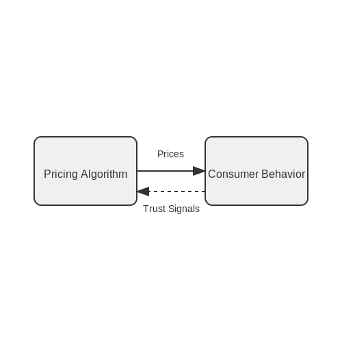
The diagram below illustrates the feedback loop between pricing algorithms and consumer trust:
5. E-Commerce: Personalized Pricing in Retail
E-Commerce: Personalized Pricing in Retail
Foundations of Dynamic Pricing
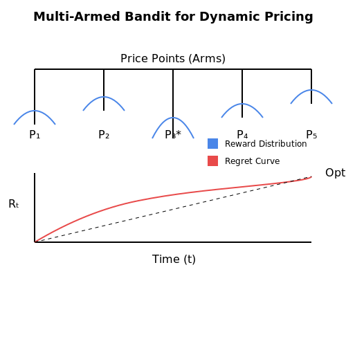
Dynamic pricing in e-commerce leverages real-time data to adjust prices based on buyer behavior, demand fluctuations, and market conditions. The core mechanism relies on machine learning models that process historical transaction data, user browsing patterns, and competitor pricing. A fundamental approach involves formulating the problem as a multi-armed bandit, where each arm represents a potential price point, and the goal is to maximize revenue while minimizing regret.
Here, Rt represents the cumulative regret at time t, Pi* is the optimal price, and Pi is the chosen price. The objective is to minimize Rt over time.
Behavioral Segmentation and Price Elasticity
Buyer behavior is segmented using clustering algorithms such as k-means or Gaussian Mixture Models (GMMs), where features include purchase frequency, cart abandonment rate, and responsiveness to discounts. Price elasticity, a critical metric, is derived via regression analysis:
where Ed is the elasticity of demand, %ΔQd is the percentage change in quantity demanded, and %ΔP is the percentage change in price. Elasticity estimates guide personalized pricing by identifying segments willing to pay premium prices versus those sensitive to minor price changes.
Reinforcement Learning for Adaptive Pricing
Reinforcement Learning (RL) frameworks, particularly Q-learning and Deep Q-Networks (DQNs), are employed to optimize pricing strategies. The state space includes user demographics, browsing history, and inventory levels, while actions correspond to price adjustments. The reward function is defined as:
where λ balances immediate revenue against long-term customer retention. Policy gradients or actor-critic methods are often used to handle high-dimensional state spaces.
Real-World Implementation Challenges
Practical deployment faces hurdles such as data sparsity for new products (cold-start problem) and ethical concerns over price discrimination. Techniques like transfer learning mitigate cold starts by leveraging data from similar products, while fairness constraints in the RL objective ensure equitable pricing across demographics.
Case Study: Amazon’s Dynamic Pricing Engine
Amazon’s system processes over 2.5 million price updates daily, using a hybrid model combining collaborative filtering for demand prediction and Thompson sampling for exploration-exploitation trade-offs. Key metrics include:
- Price Change Velocity: Frequency of adjustments (e.g., every 10 minutes for high-demand items).
- Competitor Price Weighting: Competitor data contributes 30-40% to the pricing decision.
The system’s success hinges on real-time data pipelines and microsecond-latency model inference, ensuring prices reflect the latest market dynamics.
5.2 Ride-Sharing: Surge Pricing Mechanisms
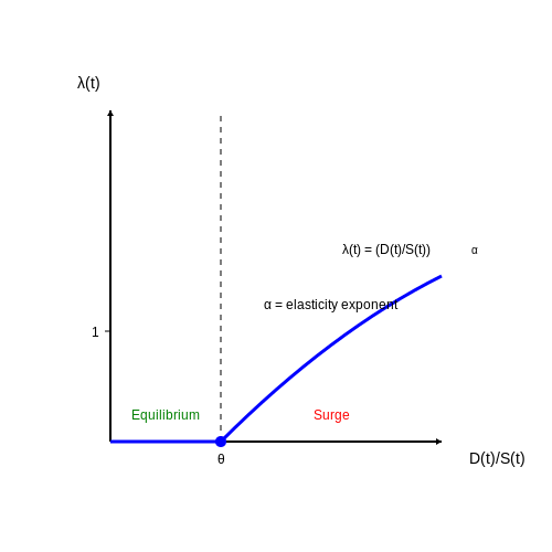
Surge pricing in ride-sharing platforms like Uber and Lyft operates as a real-time dynamic pricing mechanism designed to balance supply and demand. The core principle relies on adjusting prices multiplicatively based on the instantaneous ratio of ride requests to available drivers in a given geographic zone. Let D(t) denote demand (ride requests per unit time) and S(t) supply (available drivers) at time t. The surge multiplier λ follows a piecewise function:
where θ represents the platform-specific demand-supply equilibrium threshold (typically 0.8-1.2), and α is the elasticity exponent (usually 0.5-1.0) controlling how aggressively prices scale with imbalance. The ceiling operator ensures discrete pricing tiers for psychological acceptability.
Algorithmic Implementation
Modern implementations use a modified Thompson sampling approach to dynamically adjust θ and α. For each pricing zone z, the system maintains Beta-distributed priors over these parameters:
The posterior distributions are updated hourly using Bayesian inference on three key metrics: (1) ride fulfillment rate, (2) driver retention rate, and (3) price elasticity observed during the surge period. This allows the system to automatically adapt to regional behavioral patterns—for example, lowering α in price-sensitive markets while increasing it in time-sensitive business districts.
Spatiotemporal Considerations
Surge pricing incorporates spatial smoothing through Gaussian kernel density estimation across adjacent zones. The effective surge multiplier λ'(t) for zone i becomes:
where σ controls the smoothing radius (typically 0.5-2 km). Temporal hysteresis is implemented via an exponentially weighted moving average of demand-supply ratios to prevent rapid price fluctuations that could erode user trust.
Behavioral Economics Integration
Advanced systems incorporate prospect theory to model user reactions. The perceived value V of a surge price follows:
where γ ≈ 0.65 and δ ≈ 0.85 capture loss aversion, while κ ≈ 2.25 quantifies the stronger negative reaction to price surges compared to positive reactions to discounts. Platforms use this to optimize surge notification timing and framing.
5.3 Hospitality: Dynamic Room Rate Optimization
Revenue Management Foundations
Dynamic pricing in hospitality leverages stochastic demand models to optimize room rates. The core objective is to maximize expected revenue R over a booking horizon T, where:
Here, pt represents the price at time t, dt(pt) is the price-dependent demand function, and ct denotes remaining capacity. The bid-price control method solves this by maintaining threshold values for each inventory unit:
Demand Learning with Bayesian Methods
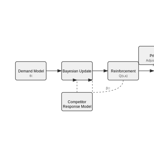
Hotels face non-stationary demand patterns influenced by seasonality and events. A hierarchical Bayesian model updates demand estimates in real-time:
where θt represents latent demand parameters, α controls the adaptation rate, and σ2 models uncertainty. The posterior distribution is updated via Markov Chain Monte Carlo (MCMC) sampling when new booking data arrives.
Competitive Price Response Modeling
In oligopolistic markets, Nash equilibrium conditions must be considered. The generalized Lotka-Volterra equations model competitor reactions:
where βij captures cross-price elasticity between hotel i and competitor j, and Ki represents market capacity. This system is solved numerically using Runge-Kutta methods.
Implementation with Reinforcement Learning
Deep Q-Networks (DQN) optimize pricing policies by learning a value function Q(s,a) that maps state s (occupancy, competitor rates) to action a (price adjustment). The Bellman equation is approximated via:
where η is the learning rate and γ the discount factor. Double DQN architectures prevent overestimation by decoupling action selection and evaluation.
Feature Engineering for Price Sensitivity
Key predictive features include:
- Lead time: Exponential decay weighting for early bookings
- Price elasticity: Calculated via historical booking gradients
- Event indicators: Binary flags for conferences/holidays
Real-World Deployment Challenges
Production systems must handle:
- Partial observability: Competitor rates scraped with noise
- Constraint satisfaction: Minimum stay requirements encoded as MIP constraints
- Explainability: SHAP values justify price recommendations to managers
Marriott International's implementation achieved 3-5% revenue lift by combining ensemble forecasting with Thompson sampling for price exploration.
6. Key Academic Papers and Research
6.1 Key Academic Papers and Research
- Dynamic Pricing Models and Negotiating Agents: Developments in ... — Linking decision systems, negotiating agents, management accounting, and computational accounting, this paper aims at exploring dynamic pricing strategies of a synthetic business-to-consumer online operation and a comparative analysis of evolving strategy-specific pricing optimization. Five price models based on market, utility, or demand information (three single and two combined), merging ...
- Dynamic Pricing with Online Reviews - SSRN — Further, we demonstrate the impact of the quality-based and value-based review models on key structural properties of the optimal pricing policies. These structural insights are also elucidated in an illustrative simulation study based on data from an online marketplace. Key words: dynamic pricing; online reviews; social learning; e-commerce ...
- Dynamic pricing and learning: Historical origins, current research, and ... — This consideration is a main driver of research on dynamic pricing and learning: the study of optimal dynamic pricing in an uncertain environment where characteristics of consumer behavior can be learned from accumulating sales data.
- PDF Designing a Dashboard to Support the Decision Process of Dynamic Pricing — Competitors-based, Cost-based, Micro-marketing and Algorithmic pricing). In addition, methods (such as Regression and Bayesian), techniques (Machine learning algorithm technique) and approaches (Conservative approach) applied for those strategies have been identified. However, the re-search on dynamic pricing for wholesale companies is still scarce and specific design rules (decision processes ...
- Pricing in consumer digital markets: A dynamic framework — Attention is now needed on conceptual work that integrates existing research and provides a dynamic pricing framework for managing ongoing customer relationships in digital markets. It is here that this paper contributes by proposing a new conceptual framework for participative pricing.
- How Does Dynamic Pricing Affect Customer Behavior on Retailing ... — PDF | On Jan 1, 2017, Dennis Zhang and others published How Does Dynamic Pricing Affect Customer Behavior on Retailing Platforms? Evidence from a Large Randomized Experiment on Alibaba | Find ...
- PDF Competition-Based Dynamic Pricing in Online Retailing: A Methodology ... — eld experiment with randomized prices. We resolve the second issue by exploiting the retailer's own and ors' stockouts as itors' prices. We estima from multiple retailers. Based on the estimates, we propose a best-response pricing strategy that takes into ount consumer choice behavior, competitors' a nd manufacturer price restrict
- PDF SJNW770-06-NO00007372 - Springer — Abstract In this paper, we use reinforcement learning (RL) techniques to determine dynamic prices in an electronic monopolistic retail market. The market that we consider consists of two natural segments of customers, captives and shoppers. Captives are mature, loyal buyers whereas the shoppers are more price sensitive and are attracted by sales promotions and volume discounts. The seller is ...
- Dynamic Pricing | SpringerLink — Dynamic pricing models based on discrete choice literature have been an active area of research, in particular within the field of revenue management. Here, suppliers aim to maximize their expected revenue by setting prices and facing discrete choice demand of consumers.
- (PDF) Dynamic Pricing with Online Reviews - ResearchGate — This paper investigates how the pricing policy of a revenue-maximizing monopolist is influenced by the social learning dynamics of customers who use online reviews to estimate the quality of the ...
6.2 Industry Reports and Whitepapers
- PDF Dynamic Pricing in the Presence of Social Learning and Strategic Consumers — 1 See Li et al. (2014) for empirical evidence of strategic consumer behavior in the air-travel industry. 1. 2 Papanastasiou and Savva Aviv and Pazgal 2008, Besbes and Lobel 2014, Cachon and Feldman 2015, Mersereau and Zhang ... 2 Pre-announced dynamic pricing is commonly employed in practice indirectly; for instance, rms may set a regular
- Dynamic pricing of electronic products with consumer reviews — Electronic products, such as digital cameras, smartphones, and DVDs, constitute the most vibrant parts of the world's economy. For example, the global smartphones market is estimated to reach $$150.3 billion in 2014 from about $$55.4 billion in 2009. 1 Electronic products share two prominent features: quality uncertainty and short life cycles. Quality uncertainty is due to the fact that ...
- Algorithmic pricing: Effects on consumer trust and price search — Companies frequently rely on pricing algorithms to automate their price setting in online markets (Fisher et al., 2018); thus, algorithmic dynamic pricing (ADP) has become a common pricing practice in the digital era, with retailers regularly tweaking products' prices in their online shops (Eley, 2019).On Amazon.com, for example, millions of price changes occur on a daily basis ...
- Dynamic Pricing: What It Is & Why It's Important | HBS Online — What Is Dynamic Pricing? Dynamic pricing is a strategy that bases products or services' prices on evolving market trends, such as:. Supply and demand; Competitor pricing; Inventory levels; Digital platforms use data analytics and technologies like artificial intelligence and machine learning to deploy sophisticated algorithms that analyze market conditions and predict optimal pricing.
- PDF A Roadmap to Becoming a Dynamic Pricing Retailer — referred to as consumer-based dynamic pricing (in the following, I will refer to this practice as "personalized pricing" to differentiate it from dynamic pricing clearly). Media reports observed that the price for a monitor in an online shop depended on how the reporter accessed the online shop, either directly or via a price comparison portal.
- PDF Dynamic Pricing for Electronic Products' - IJRPR — 5. Machine Learning for Dynamic Pricing in e-Commerce Delving into the dynamic pricing landscape in e-commerce, this paper proposes a dynamic pricing algorithm that adapts to changing market conditions, customer behaviors, and competitors' prices. By leveraging machine learning methods, especially reinforcement 13 learning, the study explores both
- Dynamic Pricing: Trends, Challenges and New Frontiers — Modern dynamic pricing has emerged as a computer-automated strategy that has revolutionized pricing methodologies and consumer interactions across various industries. This paper delves into the intricate domain of dynamic pricing, presenting an overview of its significance and the complex factors influencing its implementation. Within the realms of computer science, this subject involves ...
- Dynamic pricing with reference price effects in integrated online and ... — This article fills the gap by offering an analytical model of intertemporal price setting for dual channel pricing problem. We present an optimal control framework of dynamic pricing when (1) consumer behaviour is prone to a reference price and (2) the online channel is subject to the last-mile delivery cost.
- PDF Robust Dynamic Pricing With Strategic Customers — pricing mechanism is, for all intents, near optimal. 1. Introduction Applications of revenue management run the gamut from dynamic pricing in the airline industry, to hospitality, to retail. The following dynamic pricing problem is one of the canonical problems in revenue management: A seller is endowed with an inventory of a single product ...
- How Does Dynamic Pricing Affect Customer Behavior on Retailing ... — The essence of dynamic pricing involv es changing prices based on algorithms that take into accoun t internal factors (e.g., inven tory , shipping terms) and external * The first two authors ...
6.3 Recommended Books and Online Resources
- (PDF) Competition-Based Dynamic Pricing in Online Retailing: A ... — We estimate an empirical model capturing consumer choices among substitutable products from multiple retailers. Based on the estimates, we propose a best-response pricing strategy that takes into account consumer choice behavior, competitors' actions, and supply parameters (procurement costs, margin target, and manufacturer price restrictions).
- Algorithmic pricing: Effects on consumer trust and price search — With the widespread use of pricing algorithms in online markets, prices are increasingly fluctuating, contradicting consumers' desire for price stability. This research examines the central form of algorithmic pricing in online markets—namely, algorithmic dynamic pricing (ADP). In five studies, including one real-world ADP encounter and four incentive-based experimental studies (in ...
- PDF Competition-Based Dynamic Pricing in Online Retailing: A Methodology ... — Field Experiments to Test Price Elasticities and the Best Response Pricing Algo-rithm. A number of recent studies have used experiments to examine consumer response to price and other product attributes in di erent contexts. For example, Karlan and Zinman (2009) analyze these relationships in the context of direct mail o ers; Ashraf et al ...
- Dynamic Pricing | SpringerLink — Recently, there is growing interest and need for dynamic pricing algorithms, especially, in the field of online marketplaces by offering smart pricing options for big online stores. The dynamic adjustment of prices attracts researchers and practitioners from...
- Pricing in consumer digital markets: A dynamic framework — Attention is now needed on conceptual work that integrates existing research and provides a dynamic pricing framework for managing ongoing customer relationships in digital markets. It is here that this paper contributes by proposing a new conceptual framework for participative pricing.
- Digital Pricing: A Guide to Strategic Pricing for the Digital Economy ... — This is one of the first books to combine the current megatrend of digitalization and pricing as the most effective lever for increasing and sustaining profits. The book presents the basics of digital pricing as well as modeling methods and implementation examples. This structure helps in tackling the latest developments and challenges due to digitalization. Readers will gain a detailed ...
- Pricing in Consumer Digital Markets: A Dynamic Framework — Attention is now needed on conceptual work that integrates existing research and provides a dynamic pricing framework for managing ongoing customer relationships in digital markets. It is here that this paper contributes by proposing a new conceptual framework for participative pricing.
- PDF A Simulation-based Approach to Dynamic Pricing — As dynamic pricing systems become necessary as a competitive maneuver and as market mechanisms become large scale and more complex, there is a growing need for pricing agents to be used to automate dynamic pricing, which challenges sellers to improve their understanding of what are the best agent pricing strategies for their marketplaces.
- PDF Dynamic Pricing - DiVA — This thesis will exclusively treat customer's online service satisfaction, since dynamic pricing relies on algorithms and databases that analyze customers' online behavior and update prices accordingly.
- Dynamic Demand and Pricing Strategy in E-book Market a Dissertation — subsequent book purchases, including quantity, reading format (e-book or print book), s (Amazon, othe ine bookstores) in a number of book genres. The estimation reveals two consumer types, avid readers and general elect into b . Compared with general readers, avid readers buy more bo e-readers earlier, and have larger cannibalization rates.