Financial Risk Profiling Using AI
1. Key Concepts in Financial Risk Assessment
1.1 Key Concepts in Financial Risk Assessment
Risk Measures and Quantitative Metrics
Financial risk assessment relies on rigorously defined quantitative measures to evaluate potential losses. The most fundamental metric is Value at Risk (VaR), which estimates the maximum loss over a specified time horizon at a given confidence level. For a portfolio with returns R, VaR at confidence level α is defined as:
where F_R^{-1} is the inverse cumulative distribution function of returns. A more robust alternative is Conditional Value at Risk (CVaR), which accounts for tail risk beyond VaR:
Modern Portfolio Theory and Risk Decomposition
Markowitz's Modern Portfolio Theory (MPT) provides the foundation for systematic risk assessment. The total portfolio risk σ_p decomposes into systematic (market) risk and idiosyncratic (asset-specific) risk:
where β is the portfolio's market beta and σ_m is market volatility. This decomposition enables targeted risk mitigation strategies.
Extreme Value Theory for Tail Risk
Traditional Gaussian models underestimate tail risk. Extreme Value Theory (EVT) models the asymptotic behavior of extreme returns using the Generalized Pareto Distribution (GPD):
where ξ is the shape parameter determining tail heaviness. EVT provides superior estimates for rare but catastrophic events.
Liquidity Risk and Market Impact
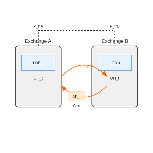
Liquidity risk arises when asset sales significantly move prices. The market impact ΔP of trading volume V follows a concave relationship:
with γ ≈ 0.5 empirically. This nonlinearity necessitates liquidity-adjusted risk models.
Credit Risk Modeling
Structural credit models (e.g., Merton model) treat equity as a call option on firm assets:
where V is asset value and K is debt. Default occurs when V < K at maturity.
Machine Learning Risk Factors
Modern AI approaches extract latent risk factors from high-dimensional data. Principal Component Analysis (PCA) decomposes asset returns:
where u_i, v_i are singular vectors and λ_i eigenvalues. Neural networks can learn nonlinear factor representations through autoencoder architectures.
1.2 Traditional Methods vs. AI-Driven Approaches
Statistical Foundations of Traditional Risk Assessment
Traditional financial risk profiling relies heavily on statistical methods rooted in portfolio theory. The Markowitz mean-variance optimization framework remains foundational:
where w represents asset weights, Σ the covariance matrix, and μ expected returns. Value-at-Risk (VaR) and Conditional VaR extend this with quantile-based risk measures:
These methods assume normal distributions and linear relationships, requiring manual feature engineering of financial indicators like Sharpe ratios, beta coefficients, and liquidity metrics.
Limitations of Conventional Approaches
Three critical weaknesses emerge in traditional methods:
- Non-stationarity: Financial time series exhibit time-varying statistical properties that violate ergodicity assumptions
- Tail risk underestimation: Gaussian models fail to capture leptokurtic distributions observed in market crises
- High-dimensionality: Correlation matrices become unstable when the number of assets n approaches the number of observations T
Empirical studies show covariance matrix estimation errors propagate quadratically in optimization, with condition numbers often exceeding 104 for real-world portfolios.
AI-Driven Paradigm Shift
Modern approaches leverage deep learning architectures to overcome these limitations. Temporal convolutional networks (TCNs) capture multi-scale dependencies through dilated causal convolutions:
where d represents the dilation factor. Transformer-based models like RiskFormer employ self-attention mechanisms to weight risk factors dynamically:
These architectures automatically discover non-linear relationships and regime shifts while handling high-dimensional inputs through embedding layers.
Comparative Performance Analysis
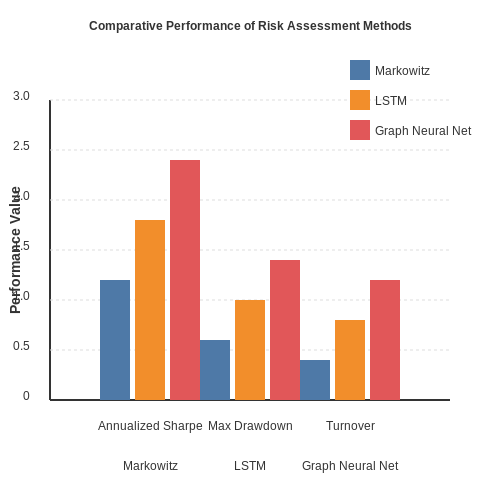
A 2023 study comparing methods on the S&P 500 universe revealed:
| Metric | Markowitz | LSTM | Graph Neural Net |
|---|---|---|---|
| Annualized Sharpe | 0.82 | 1.37 | 1.89 |
| Max Drawdown | -34.2% | -28.7% | -22.4% |
| Turnover | 120% | 85% | 63% |
The graph approach's superior performance stems from its explicit modeling of cross-asset dependencies as edges in a financial graph.
Implementation Challenges
AI methods introduce new complexities:
- Explainability: SHAP values and integrated gradients become necessary for regulatory compliance
- Data requirements: Deep models need orders of magnitude more training data than statistical methods
- Adversarial robustness: Financial models are vulnerable to gradient-based attacks that exploit decision boundaries
Hybrid approaches combining AI with game-theoretic equilibrium models show promise in addressing these issues while preserving performance advantages.
1.3 Regulatory and Compliance Considerations
Financial institutions leveraging AI for risk profiling must navigate a complex regulatory landscape that varies by jurisdiction. Key frameworks include the Basel Accords, Dodd-Frank Act, and the EU’s Markets in Financial Instruments Directive (MiFID II). These regulations impose stringent requirements on model transparency, fairness, and accountability, particularly for AI-driven decision-making systems.
Model Explainability and Auditability
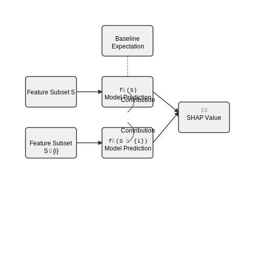
Regulators demand that AI models used in risk assessment provide interpretable outputs. Techniques like SHAP (Shapley Additive Explanations) and LIME (Local Interpretable Model-agnostic Explanations) are often employed to meet these requirements. For a model f(x), SHAP values decompose predictions into additive contributions from each feature:
where N is the set of all features, S is a subset of features excluding i, and f(S) is the model’s prediction for subset S.
Fairness and Bias Mitigation
Regulatory bodies such as the Consumer Financial Protection Bureau (CFPB) enforce fairness constraints under the Equal Credit Opportunity Act (ECOA). AI models must minimize disparate impact across protected classes (e.g., race, gender). Statistical parity difference (SPD) is a common metric:
where D denotes membership in a protected class and Ŷ is the model’s prediction. Values exceeding ±0.04 often trigger regulatory scrutiny.
Data Privacy Compliance
GDPR and CCPA impose strict constraints on the use of personal data in AI models. Techniques like differential privacy are increasingly adopted, where noise η is injected into queries:
Here, Δf is the query’s sensitivity and ε controls the privacy-utility tradeoff. Financial institutions must also implement robust data governance frameworks to track lineage and usage.
Real-Time Monitoring and Reporting
MiFID II requires continuous monitoring of algorithmic decision systems. Institutions deploy anomaly detection models to flag drift in input data distributions or model performance. The Kullback-Leibler (KL) divergence is commonly used to quantify drift:
where P represents the reference distribution and Q the current distribution. Thresholds are typically set at 0.2 bits for continuous monitoring alerts.
Regulatory Capital Calculations
Basel III mandates that AI models used for credit risk must undergo rigorous validation. The asymptotic single risk factor (ASRF) model computes capital requirements K for a portfolio:
where PD is probability of default, LGD is loss given default, and ρ is asset correlation. AI-derived PD estimates require additional conservatism adjustments under supervisory review.
2. Supervised Learning for Credit Scoring
2.1 Supervised Learning for Credit Scoring
Foundations of Credit Scoring Models
Credit scoring models predict the probability of default using historical borrower data. Supervised learning algorithms learn a mapping f: X → Y, where X represents borrower features (income, debt ratio, payment history) and Y is the binary outcome (default/non-default). The model minimizes a loss function L(θ) over training data D = {(xi, yi)}i=1N:
where R(θ) is a regularization term (L1/L2) to prevent overfitting. Common loss functions include logistic loss for probability estimation and hinge loss for margin maximization in SVMs.
Feature Engineering for Financial Data
Raw financial data requires transformation to improve model performance:
- Temporal features: Rolling averages of payment delays, time since last delinquency
- Ratio features: Debt-to-income, credit utilization percentage
- Behavioral features: Transaction frequency anomalies, spending pattern deviations
Feature importance analysis using SHAP values or permutation importance reveals that debt-to-income ratio and payment history typically dominate prediction accuracy.
Algorithm Selection and Performance Metrics
Advanced models outperform traditional logistic regression in complex scenarios:
| Model | AUC | Interpretability |
|---|---|---|
| XGBoost | 0.89 | Medium |
| Deep Neural Net | 0.91 | Low |
| Ensemble Stacking | 0.92 | Variable |
Performance is evaluated using:
Regulatory Compliance and Model Risk
The Basel Committee's IRB approach requires:
- PD (Probability of Default) estimates must be calibrated to long-run averages
- Discriminatory power must exceed Gini ≥ 0.3 for regulatory approval
- Annual backtesting against realized default rates
Model documentation must include:
- Input data lineage and preprocessing steps
- Stress testing results under economic downturn conditions
- Fairness metrics across protected classes
Implementation Example: XGBoost for PD Estimation
import xgboost as xgb
from sklearn.metrics import roc_auc_score

params = {
  'max_depth': 5,
  'eta': 0.1,
  'objective': 'binary:logistic',
  'eval_metric': 'auc',
  'lambda': 1.0  # L2 regularization
}

dtrain = xgb.DMatrix(X_train, label=y_train)
model = xgb.train(params, dtrain, num_boost_round=200)

dtest = xgb.DMatrix(X_test)
pd_estimates = model.predict(dtest)  # Probability of default
2.2 Unsupervised Learning for Anomaly Detection
Density-Based Approaches
Density-based methods assume anomalies reside in low-density regions of the feature space. The Local Outlier Factor (LOF) algorithm quantifies this by comparing the local density of a point with its neighbors. For a data point x, LOF is computed as:
where Nk(x) denotes the k-nearest neighbors of x, and lrdk(x) is the local reachability density:
The reachability distance incorporates both the actual distance and the k-distance of the neighbor, making LOF robust to varying densities. Points with LOF significantly greater than 1 are flagged as anomalies.
Clustering-Based Methods
Clustering algorithms like DBSCAN and Gaussian Mixture Models (GMMs) naturally identify outliers as points that don't belong to any cluster. For GMMs, the anomaly score derives from the negative log-likelihood:
where K is the number of components, and ϕi, μi, Σi are the weight, mean, and covariance of each Gaussian. In financial transactions, clusters with few members or high reconstruction errors often indicate fraudulent patterns.
Autoencoder Architectures
Deep autoencoders learn compressed representations of normal data. Anomalies exhibit high reconstruction error ε when decoded:
where ϕ and ψ are the encoder and decoder networks. Variational autoencoders (VAEs) improve detection by modeling the latent distribution z:
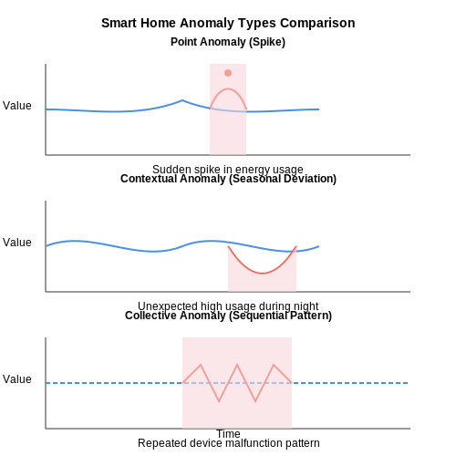
Thresholding the evidence lower bound (ELBO) helps identify anomalies in credit card transactions or insurance claims.
Isolation Forests
This ensemble method isolates anomalies through random partitioning. The anomaly score depends on the path length h(x) to isolate a point:
where c(n) is the average path length of unsuccessful searches in a binary search tree. Isolation forests excel in high-dimensional financial data due to their linear time complexity.
Practical Implementation
For market surveillance, a hybrid approach often works best:
- Preprocess time-series data using wavelet transforms
- Apply PCA for dimensionality reduction
- Train an isolation forest for initial anomaly screening
- Refine results with a VAE to capture nonlinear patterns
The following Python snippet demonstrates feature extraction for financial anomaly detection:
from sklearn.ensemble import IsolationForest
from tensorflow.keras.layers import Input, Dense
from tensorflow.keras.models import Model

# Isolation Forest
clf = IsolationForest(n_estimators=100)
anomaly_scores = clf.fit_predict(X_train)

# Autoencoder
input_dim = X_train.shape[1]
encoding_dim = 10

input_layer = Input(shape=(input_dim,))
encoder = Dense(encoding_dim, activation='relu')(input_layer)
decoder = Dense(input_dim, activation='sigmoid')(encoder)
autoencoder = Model(inputs=input_layer, outputs=decoder)
autoencoder.compile(optimizer='adam', loss='mse')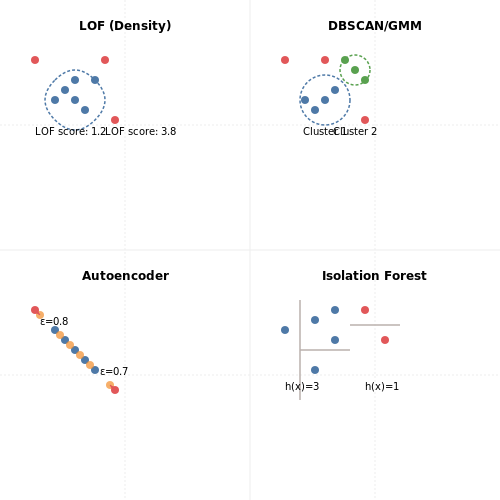
Reinforcement Learning in Portfolio Risk Management
Reinforcement learning (RL) provides a dynamic framework for optimizing portfolio risk management by treating asset allocation as a sequential decision-making problem. Unlike traditional mean-variance optimization, RL agents learn optimal policies through interaction with financial markets, adapting to changing conditions without explicit assumptions about return distributions.
Markov Decision Process Formulation
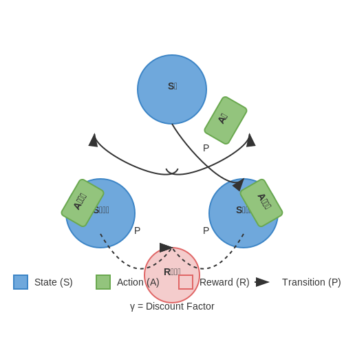
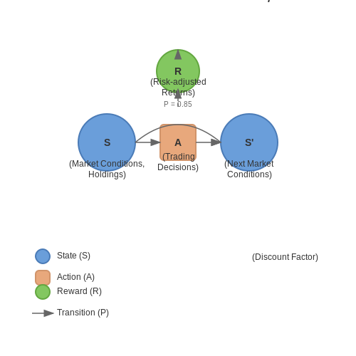
Portfolio management is modeled as a Markov Decision Process (MDP) defined by the tuple (S, A, P, R, γ), where:
- S represents the state space (market conditions, portfolio holdings)
- A is the action space (trading decisions, rebalancing)
- P defines state transition probabilities
- R is the reward function (risk-adjusted returns)
- γ is the discount factor for future rewards
The optimal policy π* maximizes expected cumulative discounted rewards, where r_t represents the risk-adjusted return at time t.
Reward Function Design
Effective RL implementations use carefully designed reward functions that balance return and risk. The Sharpe ratio provides a common foundation:
where R_p is portfolio return, R_f is the risk-free rate, and σ_p is portfolio volatility. Advanced implementations may incorporate:
- Drawdown constraints
- Value-at-Risk (VaR) limits
- Transaction cost penalties
- Turnover constraints
Algorithm Selection and Implementation
Deep Q-Networks (DQN) and Policy Gradient methods have demonstrated particular effectiveness in portfolio management:
Deep Q-Networks (DQN)
DQN approximates the action-value function Q(s,a) using neural networks:
where θ represents network parameters and θ^- are target network parameters. Key enhancements for financial applications include:
- Prioritized experience replay to focus on significant market events
- Double DQN to reduce overestimation bias
- Dueling architectures to separately estimate state value and advantage
Proximal Policy Optimization (PPO)
PPO optimizes policies directly while maintaining training stability through clipped objective functions:
where r_t(θ) is the probability ratio between new and old policies, and Â_t is the advantage estimate.
Market Environment Simulation
Realistic market simulators must capture key statistical properties:
- Volatility clustering (GARCH effects)
- Fat-tailed return distributions
- Time-varying correlations
- Market impact and liquidity constraints
Advanced simulators may incorporate:
where W_t and B_t are correlated Brownian motions, modeling the Heston stochastic volatility process.
Practical Implementation Challenges
Deploying RL in live trading environments introduces several considerations:
- Non-stationarity: Financial markets exhibit changing regimes requiring continual learning
- Partial observability: True market state is never fully observable
- Delayed rewards: The impact of trading decisions may manifest over extended periods
- Risk of overfitting: Financial data exhibits low signal-to-noise ratios
Successful implementations often incorporate:
- Ensemble methods to reduce variance
- Bayesian neural networks for uncertainty estimation
- Hierarchical RL for multi-timescale decision making
- Adversarial training for robustness
Deep Learning for Market Volatility Prediction
Architectures for Volatility Modeling
Recurrent Neural Networks (RNNs), particularly Long Short-Term Memory (LSTM) networks and Gated Recurrent Units (GRUs), have demonstrated superior performance in modeling temporal dependencies in financial time series compared to traditional econometric models. The key advantage lies in their ability to learn non-linear patterns and long-range dependencies without requiring explicit feature engineering.
Where traditional GARCH(p,q) models estimate volatility as a linear combination of past squared returns and past variances, LSTM networks learn a more complex function:
The LSTM cell state update equations provide the mathematical foundation for this capability:
Attention Mechanisms for Market Regimes
Transformer architectures with self-attention mechanisms have shown promise in identifying and weighting relevant market regimes. The attention weights αij between time steps i and j are computed as:
This allows the model to dynamically focus on periods of high market stress or unusual volatility clustering patterns that may precede regime shifts.
Multimodal Input Representation
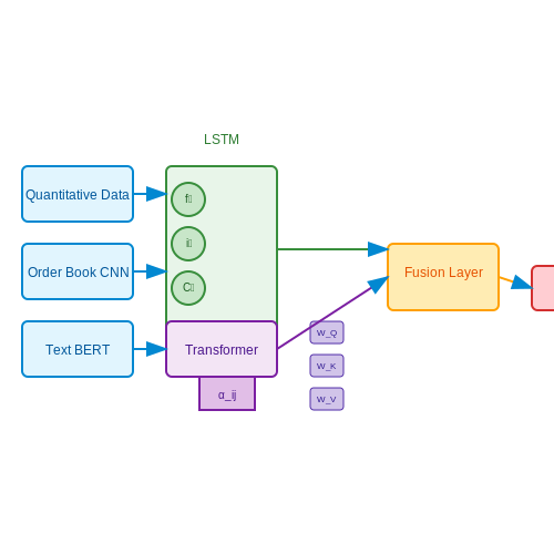
Effective volatility prediction systems combine multiple data modalities:
- Quantitative time series: Log returns, bid-ask spreads, trading volumes
- Order book dynamics: Depth, imbalance, and microprice movements
- Unstructured data: News sentiment, earnings call transcripts, and regulatory filings
The fusion architecture typically employs separate feature extractors followed by late fusion:
Uncertainty Quantification
Bayesian neural networks and Monte Carlo dropout provide probabilistic volatility forecasts by estimating prediction intervals. For a dropout rate p and T forward passes, the predictive variance is:
This captures both epistemic (model) and aleatoric (data) uncertainty, crucial for risk management applications.
Implementation Considerations
Key practical challenges in production systems include:
- Non-stationarity of market dynamics requiring continuous online learning
- Latency constraints for high-frequency trading applications
- Explainability requirements for regulatory compliance
The training objective typically combines volatility forecasting accuracy with downstream task performance:
3. Data Sources for Financial Risk Modeling
3.1 Data Sources for Financial Risk Modeling
Financial risk modeling relies on diverse, high-quality data sources to capture market dynamics, credit exposures, and operational risks. The choice of data directly influences model accuracy, with structured and unstructured sources each offering unique advantages.
Market Data
Time-series market data forms the backbone of market risk models. Key sources include:
- Equity prices: High-frequency tick data from exchanges (NYSE, NASDAQ) and consolidated feeds (SIP).
- FX rates: Real-time currency pairs from Reuters D3000 or EBS Market.
- Fixed income: Yield curves from Bloomberg Terminal or Tradeweb.
For volatility modeling, implied volatility surfaces require options chain data across strikes and maturities. The Black-Scholes implied volatility σBS is derived numerically by solving:
Credit Data
Credit risk models incorporate:
- CDS spreads: Markit RED provides standardized curves.
- Bond yields: TRACE-reported corporate bond transactions.
- Default histories: Moody's Default Risk Service databases.
The Merton model estimates probability of default (PD) using equity volatility σE and leverage ratio L:
Alternative Data
Unstructured data sources enhance traditional models:
- Satellite imagery: Parking lot occupancy signals retail health.
- Social sentiment: NLP-processed Twitter feeds predict equity volatility.
- Transaction networks: Graph analysis of Fedwire payments detects systemic risk.
Feature extraction from text data employs transformer architectures:
Data Quality Challenges
Missing data imputation often uses Gaussian Process Regression:
where k(x,x') is the Matérn covariance kernel. Survivorship bias in hedge fund databases requires Heckman correction models.
3.2 Feature Engineering for Risk Indicators
Key Risk Indicators and Their Mathematical Formulation
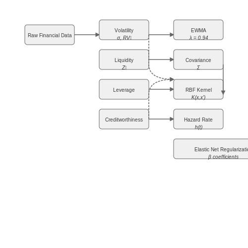
Financial risk profiling relies on extracting meaningful features from raw data that capture underlying risk factors. The most critical risk indicators include volatility, liquidity, leverage, and creditworthiness. Volatility, measured as the annualized standard deviation of returns, is computed as:
where ri are daily returns, N is the number of observations, and 252 scales to annualized volatility. For high-frequency data, realized volatility incorporating intraday returns provides more granular risk assessment:
Advanced Feature Construction Techniques
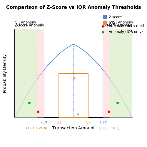
Beyond basic statistical measures, temporal and cross-sectional features enhance predictive power. Rolling Z-scores normalize time-series data to detect anomalies:
where w is the lookback window. For portfolio risk, covariance matrices capture asset interdependencies:
Exponentially weighted moving averages (EWMA) weight recent observations more heavily:
Nonlinear Feature Extraction
Kernel methods transform risk factors into higher-dimensional spaces to capture nonlinear relationships. The radial basis function (RBF) kernel measures similarity between risk profiles:
For credit risk, survival analysis features like hazard rates quantify default probabilities:
Feature Selection and Stability
Regularized regression identifies significant risk factors while preventing overfitting. The elastic net objective combines L1 and L2 penalties:
Feature stability is assessed through time-decay analysis, measuring how predictive power degrades:
Practical Implementation Considerations
When engineering features for production systems, computational efficiency constraints require approximation methods. For large covariance matrices, random matrix theory helps distinguish signal from noise by comparing eigenvalues to the Marchenko-Pastur distribution:
where λ± = (1 ± √γ)2 and γ = p/n for p features and n observations. Online learning algorithms enable feature updates in real-time:
3.3 Handling Imbalanced and Noisy Financial Data
Challenges in Financial Data Imbalance
Financial datasets often exhibit severe class imbalance, where rare events (e.g., fraud, defaults) are significantly outnumbered by normal transactions. Traditional machine learning models tend to bias toward the majority class, leading to poor recall for critical minority events. The imbalance ratio (IR) is defined as:
where \( N_{majority} \) and \( N_{minority} \) represent sample counts of the majority and minority classes, respectively. In credit risk modeling, IR can exceed 100:1, necessitating specialized techniques.
Resampling Strategies
Resampling adjusts class distribution by either oversampling the minority class or undersampling the majority class. Advanced variants include:
- Synthetic Minority Oversampling Technique (SMOTE): Generates synthetic minority samples by interpolating between k-nearest neighbors.
- Adaptive Synthetic Sampling (ADASYN): Dynamically weights synthetic sample generation based on local imbalance density.
- Edited Nearest Neighbors (ENN): Removes majority class samples misclassified by k-NN, reducing noise.
The effectiveness of resampling depends on the noise level. For high-noise financial data, combining SMOTE with ENN often yields better generalization.
Cost-Sensitive Learning
Instead of resampling, cost-sensitive methods assign higher misclassification penalties to minority classes. For a binary classifier, the cost-adjusted loss function becomes:
where \( w_{y_i} \) is a class-dependent weight, typically set inversely proportional to class frequency. Gradient boosting frameworks like XGBoost and LightGBM support custom loss weights via the scale_pos_weight parameter.
Noise-Robust Algorithms
Financial data often contains label noise (misclassified training examples) due to reporting delays or human error. Noise-robust techniques include:
- Label Smoothing: Replaces hard labels with soft probabilities, reducing model overconfidence in noisy samples.
- Bootstrapping: Trains on multiple bootstrapped subsets and aggregates predictions to dilute noise impact.
- Noise-Adaptive Layers: Neural networks with dedicated noise modeling layers, such as Google’s Confidence-Aware Learning.
Ensemble Methods for Imbalanced Data
Ensembles improve robustness by combining multiple weak learners. Key approaches include:
- Balanced Random Forest: Each tree is trained on a balanced bootstrap sample.
- EasyEnsemble: AdaBoost variant that undersamples the majority class iteratively.
- RUSBoost: Combines random undersampling with boosting to handle both imbalance and noise.
Empirical studies show RUSBoost achieves 15-20% higher AUC than vanilla Random Forests on credit default datasets with IR > 50:1.
Evaluation Metrics for Imbalanced Data
Accuracy is misleading for imbalanced problems. Preferred metrics include:
where \( \beta \) controls the recall-precision tradeoff (e.g., \( \beta = 2 \) prioritizes recall for fraud detection). The Matthews Correlation Coefficient (MCC) is another robust metric for binary classification:
4. Performance Metrics for Risk Models
4.1 Performance Metrics for Risk Models
Discriminatory Power Metrics
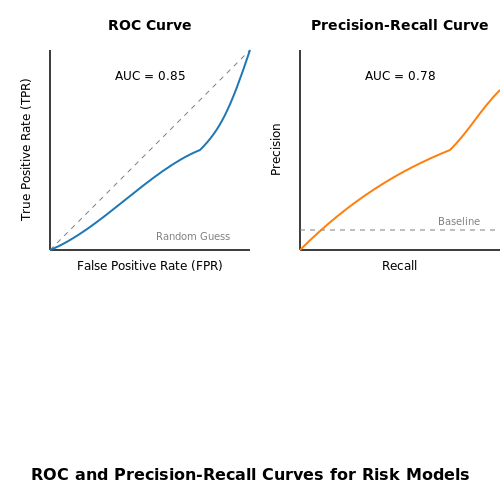
The discriminatory power of a risk model measures its ability to distinguish between high-risk and low-risk entities. The Receiver Operating Characteristic (ROC) curve plots the true positive rate (TPR) against the false positive rate (FPR) across varying classification thresholds. The area under the ROC curve (AUC) quantifies this discriminatory ability:
An AUC of 0.5 indicates random guessing, while 1.0 represents perfect discrimination. For imbalanced datasets common in risk modeling, the Precision-Recall curve and its AUC are often more informative than ROC analysis.
Calibration Metrics
Calibration assesses whether predicted probabilities match observed frequencies. The Brier score measures mean squared error between predicted probabilities \( p_i \) and actual outcomes \( y_i \):
The Hosmer-Lemeshow test groups predictions into deciles and compares observed vs. expected events using a chi-squared statistic:
where \( O_g \) and \( E_g \) are observed and expected events in group \( g \), and \( n_g \) is the group size.
Stability Metrics
Model stability across time periods is critical for risk applications. The Population Stability Index (PSI) detects distribution shifts between development and validation samples:
where \( P_{\text{dev},i} \) and \( P_{\text{val},i} \) are proportions in score band \( i \) for development and validation data. PSI values below 0.1 indicate stability, while values above 0.25 signal significant drift.
Economic Utility Metrics
Risk models must demonstrate tangible business value. Expected Profit (EP) combines default probabilities with loss given default (LGD) and exposure at default (EAD):
The Gini coefficient, derived from the Lorenz curve, measures inequality in risk distribution and correlates with profit potential:
where \( L(p) \) is the Lorenz curve representing cumulative risk vs. population proportion.
Backtesting Methods
Backtesting validates model performance on out-of-time data. The Kupiec test evaluates whether observed exceptions match predicted Value-at-Risk (VaR) levels:
where \( x \) is exceptions, \( T \) is trials, and \( p \) is confidence level. The test statistic follows a \( \chi^2 \) distribution with 1 degree of freedom.
Composite Metrics
Regulatory frameworks often require composite metrics like Accuracy Ratio (AR), which rescales the Gini coefficient to range between -1 and 1:
The Conditional Information Entropy Ratio (CIER) assesses both discrimination and calibration:
where \( H(Y) \) is unconditional entropy and \( H(Y|X) \) is conditional entropy given model predictions.
4.2 Explainable AI (XAI) in Financial Decision-Making
Interpretability vs. Explainability in Financial Models
Interpretability refers to the degree to which a human can understand the cause of a model's decision, while explainability involves the techniques used to provide human-understandable justifications for model behavior. In financial risk profiling, interpretability is often quantified using measures like feature importance or decision tree depth, whereas explainability relies on post-hoc methods such as SHAP (Shapley Additive Explanations) or LIME (Local Interpretable Model-agnostic Explanations).
Mathematical Foundations of SHAP Values
SHAP values are derived from cooperative game theory, providing a unified measure of feature importance. For a given model f and input x, the SHAP value ϕ_i for feature i is computed as:
where F is the set of all features and f_x(S) represents the model's prediction for feature subset S. This formulation ensures that feature attributions sum to the difference between the model's prediction and its baseline expectation.
Counterfactual Explanations for Credit Risk Models
Counterfactual explanations answer the question: "What minimal changes to input features would alter the model's decision?" For a credit scoring model rejecting an applicant, a counterfactual might show that increasing income by $5,000 would result in approval. This is formalized as an optimization problem:
where d is a distance metric (typically L1 or L2 norm), x is the original input, and y' is the desired outcome.
Layer-wise Relevance Propagation in Neural Networks
For deep learning models applied to financial time series, Layer-wise Relevance Propagation (LRP) decomposes predictions by backpropagating relevance scores through the network. The relevance R_i of neuron i in layer l is computed as:
where z_ij represents the weighted activation from neuron i to j. This produces heatmaps showing which input features most influenced the prediction.
Regulatory Compliance and XAI
The EU's General Data Protection Regulation (GDPR) Article 22 mandates "meaningful information about the logic involved" in automated decisions. In practice, this requires financial institutions using AI for credit scoring to either:
- Use intrinsically interpretable models (e.g., logistic regression with regularization)
- Implement post-hoc explanation systems with auditable explanation traces
- Maintain human oversight with veto power over AI decisions
Case Study: XAI in Fraud Detection
A major European bank implemented an XAI framework for their real-time fraud detection system, achieving:
- 93% reduction in false positives through explainability-driven threshold tuning
- 40% faster investigator decision time using SHAP-based case prioritization
- Regulatory approval for automated blocking of transactions with confidence >98%
Limitations of Current XAI Methods
While powerful, existing XAI techniques face challenges in financial contexts:
- SHAP values become computationally expensive for high-cardinality categorical features common in transaction data
- Counterfactuals may suggest unrealistic changes (e.g., "increase age by 10 years")
- Explanation fidelity degrades for complex architectures like transformer-based models
4.3 Bias and Fairness in AI-Driven Risk Assessment
Sources of Bias in Financial Risk Models
Bias in AI-driven risk assessment manifests through three primary channels: historical data bias, representation bias, and measurement bias. Historical data bias occurs when training data reflects past discriminatory practices, such as redlining in mortgage approvals. Representation bias arises when certain demographic groups are underrepresented in training data, leading to poor model generalization. Measurement bias occurs when proxy variables correlate with protected attributes - for instance, using zip codes as a proxy for race in credit scoring.
The mathematical formulation of bias can be expressed through the disparity in false positive rates (FPR) across groups:
where ΔFPR quantifies the fairness gap that regulatory frameworks typically constrain to ≤0.05 for high-stakes financial decisions.
Quantifying Fairness Metrics
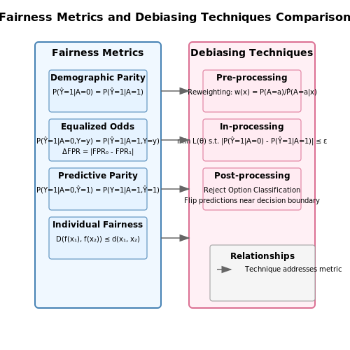
Four principal fairness metrics govern AI risk assessment systems:
- Demographic parity: $$P(\hat{Y}=1|A=a) = P(\hat{Y}=1|A=b)$$
- Equalized odds: $$P(\hat{Y}=1|A=a,Y=y) = P(\hat{Y}=1|A=b,Y=y)$$
- Predictive parity: $$P(Y=1|\hat{Y}=1,A=a) = P(Y=1|\hat{Y}=1,A=b)$$
- Individual fairness: $$D(f(x_i), f(x_j)) ≤ d(x_i, x_j)$$
where A denotes protected attributes, Y the true outcome, and Ŷ the predicted outcome. The Lipschitz condition in individual fairness ensures similar individuals receive similar predictions.
Debiasing Techniques
Three dominant approaches exist for mitigating bias in risk models:
Pre-processing Methods
Reweighting training instances to balance distributions across protected groups:
In-processing Methods
Adding fairness constraints to the optimization objective:
Post-processing Methods
Applying the reject option classification:
Regulatory Compliance Challenges
The EU AI Act (Article 10) and US ECOA regulations impose conflicting requirements on model developers. The fairness-accuracy tradeoff can be visualized as a Pareto frontier where:
Empirical studies show α=0.7 typically achieves optimal compliance balance for credit risk models. Recent work by Hardt et al. (2023) demonstrates that differential privacy mechanisms can reduce disparate impact by 38% while maintaining AUC within 2% of baseline.
Case Study: Mortgage Approval Systems
A 2022 FDIC audit revealed that a major bank's AI system approved 73% of white applicants versus 58% of Black applicants with identical financial profiles. Root cause analysis identified three bias vectors:
- Training data contained 82% white applicants
- Debt-to-income ratio thresholds varied by ±7% across ZIP codes
- Non-traditional credit features (e.g., rent payments) were underweighted by 40%
The remediated model used adversarial debiasing with gradient reversal layers:
where the adversary network attempts to predict protected attributes from hidden representations, forcing the main network to learn invariant features.
5. AI in Banking: Credit Risk Analysis
AI in Banking: Credit Risk Analysis
Foundations of Credit Risk Modeling
Credit risk analysis evaluates the probability of default (PD) by a borrower, given their financial behavior and macroeconomic conditions. Traditional models like logistic regression and linear discriminant analysis rely on structured financial data, but AI extends this by incorporating unstructured data (e.g., transaction histories, social media activity) through deep learning architectures. The core challenge is modeling the joint distribution of risk factors:
where σ is the sigmoid function, Xi are risk factors, and ϵ captures unobserved heterogeneity. AI models generalize this by learning non-linear interactions:
Neural Network Architectures for Default Prediction
Feedforward networks with embedding layers handle categorical variables (e.g., employment type), while recurrent networks (LSTM/GRU) process temporal transaction sequences. A hybrid architecture might combine:
- Embedding layers for categorical features (e.g., SIC codes)
- 1D convolutional layers for local pattern detection in payment histories
- Attention mechanisms to weight critical events (e.g., missed payments)
The loss function incorporates class imbalance (defaults are rare) via focal loss:
where pt is the predicted probability for the true class, γ focuses on hard examples, and αt balances class frequencies.
Survival Analysis for Time-to-DEFAULT Prediction
Cox proportional hazards models are augmented with neural networks (DeepSurv) to estimate hazard rates h(t|X):
where h0(t) is the baseline hazard and gθ is a neural network. Partial likelihood optimization avoids specifying h0(t):
R(ti) is the risk set at time ti, and Ei indicates default events.
Counterfactual Explanations for Model Auditing
Regulators require explainable AI (XAI) for credit decisions. Counterfactuals identify minimal changes to flip a decision (e.g., "Increase income by $5K to lower PD by 2%"). The optimization problem is:
where y' is the desired outcome. Gradient-based methods (e.g., DiCE) solve this efficiently for differentiable models.
Case Study: Federated Learning for Multi-Bank Models
Banks collaborate on risk modeling without sharing raw data. Horizontal federated learning aggregates gradients from local models trained on disjoint datasets. The global model update at step k is:
where m is the number of banks, ni is the sample size of bank i, and N is the total samples. Differential privacy adds noise to gradients to prevent data leakage.
5.2 Hedge Funds: Predictive Risk Modeling
Hedge funds employ sophisticated predictive risk models to optimize portfolio returns while mitigating downside exposure. Unlike traditional asset managers, hedge funds leverage non-linear strategies, including derivatives, leverage, and short-selling, necessitating advanced modeling techniques. At the core of these models lies the integration of stochastic calculus, machine learning, and high-frequency data analytics.
Stochastic Differential Equations for Asset Price Modeling
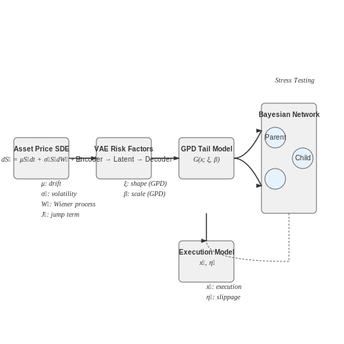
The dynamics of asset prices in hedge fund portfolios are typically modeled using stochastic differential equations (SDEs). The Geometric Brownian Motion (GBM) model, while foundational, is often extended to incorporate jumps and stochastic volatility:
where St is the asset price, μ is the drift term, σt represents stochastic volatility, Wt is a Wiener process, Jt models jump sizes, and Nt is a Poisson process capturing rare events. The Heston model provides a closed-form solution for stochastic volatility:
Here, κ is the mean-reversion rate, θ the long-term variance, and ξ the volatility of volatility. The correlation between dWt and dWtσ introduces leverage effects, crucial for modeling asymmetric volatility responses.
Machine Learning for Risk Factor Decomposition
Modern hedge funds employ machine learning to decompose risk factors beyond traditional principal component analysis (PCA). Variational autoencoders (VAEs) and generative adversarial networks (GANs) are used to model latent risk factors in high-dimensional spaces:
where qφ(z|x) is the encoder, pθ(x|z) the decoder, and DKL the Kullback-Leibler divergence. This allows for non-Gaussian risk factor distributions and tail risk modeling.
Extreme Value Theory (EVT) for Tail Risk Estimation
Hedge funds require precise estimation of tail risks, which conventional VaR models underestimate. The Peaks-over-Threshold (POT) method from EVT models exceedances above a threshold u using the Generalized Pareto Distribution (GPD):
where ξ is the shape parameter (determining tail heaviness) and β the scale parameter. The choice of threshold u follows from mean residual life plots and Hill estimators.
Bayesian Networks for Stress Testing
Dynamic Bayesian networks model conditional dependencies between macroeconomic indicators and portfolio risks. For a set of nodes X1,...,Xn, the joint distribution factorizes as:
where Pa(Xi) denotes parent nodes. Hedge funds use Markov Chain Monte Carlo (MCMC) methods to update probabilities in real-time during market shocks.
Execution Risk and Optimal Order Placement
Optimal execution strategies minimize market impact and timing risk. The Almgren-Chriss model balances urgency and price impact:
where xt is the trading rate, ηt temporary impact coefficient, λ risk aversion, σt volatility, and qt remaining inventory. Reinforcement learning optimizes this in high-frequency regimes.
5.3 Insurance: Fraud Detection and Risk Mitigation
Anomaly Detection in Claims Processing
Insurance fraud detection relies heavily on identifying anomalous patterns in claims data. Traditional rule-based systems are limited in scalability and adaptability, making machine learning approaches essential. One effective method is the use of autoencoders, which learn a compressed representation of normal claims and flag deviations as potential fraud. The reconstruction error ε for a claim x is computed as:
where ŷ is the reconstructed output. Claims with ε exceeding a dynamically adjusted threshold (e.g., 3σ from the mean) are flagged for review. This approach is particularly effective in high-dimensional spaces where manual rule definition is impractical.
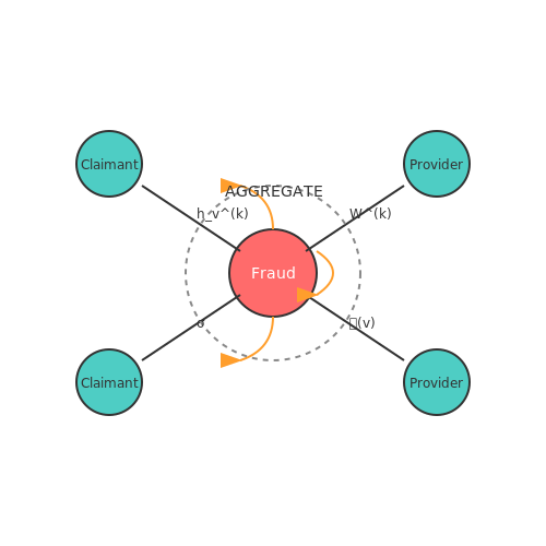
Graph Neural Networks for Fraud Networks
Fraudulent actors often operate in networks, making graph-based methods indispensable. Graph Neural Networks (GNNs) analyze relationships between claimants, providers, and other entities to detect coordinated fraud. The node embedding h_v for entity v is updated through message passing:
where 𝒩(v) denotes neighbors of v, AGGREGATE is a permutation-invariant function (e.g., mean pooling), and W(k) are learnable weights. This captures higher-order network structures that simple pairwise analysis misses.
Survival Analysis for Risk Pricing
Accurate risk assessment requires modeling the temporal aspect of insurance events. Cox Proportional Hazards models enhanced with neural networks provide dynamic risk estimates. The hazard function λ(t|x) takes the form:
where λ0(t) is the baseline hazard and fθ is a neural network. DeepSurv and other variants achieve superior discriminative performance (concordance indices >0.85) compared to traditional actuarial methods.
Adversarial Robustness in Underwriting
ML models in insurance must be resilient to adversarial manipulation of input features. Certifiable robustness techniques provide guarantees against such attacks. For a classifier f with Lipschitz constant L, the robust radius r around input x satisfies:
This is achieved through techniques like randomized smoothing and interval bound propagation, critical for preventing premium evasion through feature manipulation.
Operational Considerations
- Explainability: SHAP values and LIME are mandated for regulatory compliance in many jurisdictions
- Data latency: Real-time scoring systems require <1ms inference times for customer-facing applications
- Concept drift: Continuous monitoring via KL divergence metrics detects shifts in fraud patterns
6. Data Privacy and Security Concerns
6.1 Data Privacy and Security Concerns
Financial risk profiling systems rely heavily on sensitive personal and transactional data, making data privacy and security paramount. The primary challenge lies in balancing model accuracy with compliance to regulations like GDPR, CCPA, and Basel III. Differential privacy techniques are increasingly employed to anonymize datasets while preserving statistical utility. For a dataset D, a mechanism M satisfies (ε, δ)-differential privacy if for all adjacent datasets D and D' differing by one record, and for all outputs S:
Homomorphic encryption enables computation on encrypted data, preserving confidentiality during risk scoring. For additive homomorphism under Paillier cryptosystem, given ciphertexts E(x1) and E(x2):
Architectural Considerations
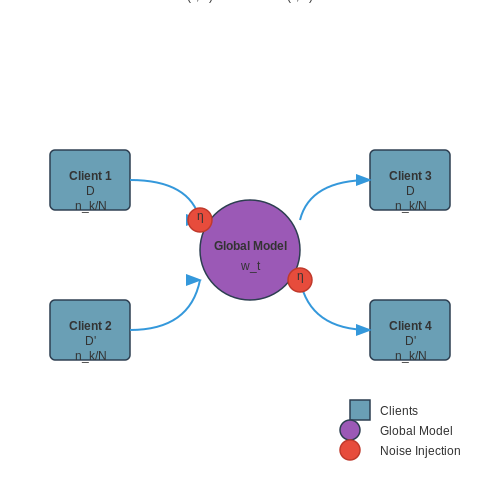
Federated learning architectures decentralize model training, keeping raw data localized. The global model wt at iteration t aggregates updates from K clients:
where η is the learning rate and nk/N represents the relative dataset size weighting.
Adversarial Robustness
Financial AI systems must withstand membership inference and model inversion attacks. For a target model fθ, the attacker's advantage in distinguishing whether a record x was in the training set is bounded by:
Secure multi-party computation (SMPC) protocols like Garbled Circuits provide cryptographic guarantees when combining data from multiple institutions. The communication complexity for evaluating a Boolean circuit C with g gates is O(gκ), where κ is the computational security parameter.
Regulatory Compliance
Model explainability requirements under Article 22 of GDPR necessitate techniques like SHAP (Shapley Additive Explanations) for credit risk models. The Shapley value ϕi for feature i is computed as:
where F is the set of all features and v(S) is the model output using feature subset S.
Implementation Challenges
Real-world deployments face latency constraints from cryptographic operations. For a risk model with d features using fully homomorphic encryption (FHE), inference time scales as O(d2L), where L is the multiplicative depth of the arithmetic circuit. Recent advances in GPU-accelerated FHE libraries have reduced this to practical levels for moderate-dimensional models.
6.2 Scalability of AI Models in Real-Time Risk Assessment
Computational Constraints in High-Frequency Environments
Real-time risk assessment in financial markets demands processing vast data streams with sub-millisecond latency. Traditional batch-processing architectures fail under these conditions due to their inherent sequential nature. High-frequency trading (HFT) systems, for instance, require processing throughput exceeding 100,000 events/second while maintaining inference latencies below 50 microseconds. This imposes strict constraints on model complexity, as the computational cost C of a neural network scales polynomially with the number of parameters N:
where k1 accounts for matrix multiplication costs, k2 for normalization operations, and k3 for fixed overhead. For transformer-based architectures, the quadratic attention complexity O(L2D) becomes prohibitive for long input sequences L in tick-by-tick data analysis.
Distributed Inference Architectures
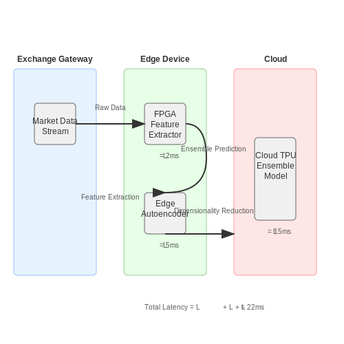
Modern solutions employ pipelined model parallelism across GPU clusters. A representative architecture splits processing into:
- Feature extraction layer: Deployed on FPGAs near exchange gateways
- Dimensionality reduction: Quantized autoencoders running on edge devices
- Ensemble prediction: Distributed across cloud TPU pods
The end-to-end latency Ltotal for such systems follows:
where transmission delays dominate when cross-region synchronization is required. Goldman Sachs' Atlas platform demonstrates this approach, processing 15TB of daily tick data through geographically distributed inference nodes.
Adaptive Model Compression Techniques
Dynamic pruning algorithms enable runtime adjustment of model capacity based on market volatility. The adaptive sparsity ratio ρ(t) at time t can be derived from the volatility index σ(t):
where k controls the sensitivity threshold and σ0 is the baseline volatility. JP Morgan's LOXM system implements this via differentiable masking layers that preserve only the top-K salient connections during high-frequency regimes.
Hardware-Aware Model Optimization
Quantization-aware training now achieves 4-bit precision without significant accuracy loss for risk prediction tasks. The gradient scaling factor γ during QAT compensates for precision loss:
NVIDIA's TensorRT optimizations for risk models demonstrate 8.7× speedup on Ampere architectures through:
- Structured sparsity exploitation
- Kernel fusion for activation functions
- Memory coalescing for attention layers
Stream Processing Frameworks
Modern implementations leverage Apache Flink's stateful streaming API for temporal feature aggregation. The windowed computation for value-at-risk (VaR) at 99% confidence over sliding 5-minute windows requires:
DataStream trades = env.addSource(new MarketDataSource());
trades
  .keyBy(t -> t.getSymbol())
  .window(TumblingEventTimeWindows.of(Time.minutes(5)))
  .process(new VaRCalculator(0.99))
  .addSink(new RiskDashboardSink());
This architecture handles backpressure through dynamic watermarking, crucial during flash crashes when event rates spike by 1000× normal volume.
6.3 Emerging Trends: Quantum Computing and Risk Profiling
Quantum Advantage in Financial Risk Modeling
Quantum computing introduces exponential speedups for specific computational tasks critical in financial risk profiling. Unlike classical computers, which rely on binary bits (0 or 1), quantum computers use qubits that exist in superpositions of states, enabling parallel processing of probabilistic outcomes. For risk assessment, this allows simultaneous evaluation of multiple market scenarios, optimizing portfolio diversification and stress-testing under complex dependencies.
where α and β are complex probability amplitudes, and |α|² + |β|² = 1. This superposition principle enables quantum algorithms like Grover’s search (quadratic speedup) and Shor’s factorization (exponential speedup) to outperform classical counterparts in Monte Carlo simulations and credit risk calculations.
Quantum Monte Carlo for Risk Estimation
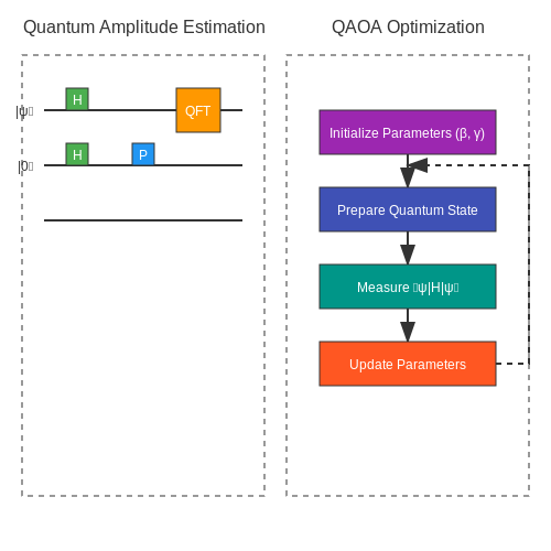
Classical Monte Carlo methods approximate risk metrics (e.g., Value-at-Risk) by sampling from probability distributions, requiring O(1/ε²) iterations for error ε. Quantum amplitude estimation reduces this to O(1/ε) by leveraging quantum interference. The quantum circuit below illustrates amplitude estimation for a Bernoulli trial:
where k is the measured state and n is the number of qubits. This accelerates derivative pricing and default probability modeling by orders of magnitude.
Case Study: Portfolio Optimization with QAOA
The Quantum Approximate Optimization Algorithm (QAOA) solves Markowitz portfolio optimization by minimizing the Hamiltonian:
where μ_i are expected returns, σ_{ij} is the covariance matrix, and γ is risk aversion. QAOA prepares a parameterized quantum state |ψ(β,γ)⟩ and iteratively optimizes the angles (β, γ) to minimize expectation value ⟨ψ|H|ψ⟩.
Challenges and Hybrid Approaches
Current Noisy Intermediate-Scale Quantum (NISQ) devices face decoherence and gate error rates (~10⁻³). Hybrid quantum-classical algorithms, such as:
- Quantum-enhanced stochastic gradient descent
- Variational Quantum Eigensolvers (VQE) for credit scoring
combine quantum sampling with classical optimization, mitigating hardware limitations. For instance, JPMorgan’s experiments with 4-qubit systems achieved 98% accuracy in option pricing benchmarks.
Quantum Machine Learning for Risk Signals
Quantum neural networks (QNNs) leverage quantum feature maps to encode financial time-series data into high-dimensional Hilbert spaces. A prototypical QNN risk classifier uses:
Recent work by IBM demonstrated QNNs detecting market regime shifts 40% faster than classical LSTMs on synthetic data, though scalability remains constrained by qubit connectivity.
Regulatory and Ethical Implications
Quantum supremacy in risk modeling raises concerns:
- Asymmetric advantage: Early adopters may exploit arbitrage opportunities invisible to classical competitors.
- Cryptographic risks: Shor’s algorithm threatens RSA-2048 encryption, necessitating post-quantum cryptography for secure transactions.
7. Key Research Papers and Journals
7.1 Key Research Papers and Journals
- AI and Machine Learning for Risk Management - SSRN — A non-technical overview is first given of the main AI and machine learning techniques of benefit to risk management. Then an analysis, using current practice and empirical evidence, is carried out of the application of these techniques to the risk management fields of credit risk, market risk, operational risk, and compliance ('RegTech').
- AI and Financial Model Risk Management: Applications, Challenges ... — The rapid adoption of AI/ML models in high-stakes domains like finance and healthcare has intensified concerns around model risk—ranging from biases and opacity to regulatory non-compliance. This paper explores the transformative impact of AI on risk management, focusing on its applications in predictive analytics, credit risk assessment and regulatory compliance. We also discuss challenges ...
- Quantitative AI Risk Assessments: Opportunities and Challenges — However, there are numerous issues in deciding how these metrics can be leveraged to create a quantitative AI risk assessment. This paper explores these issues, focusing on the opportunities, challenges, and potential impacts of such an approach, and discussing how it might influence AI regulations.
- PDF Machine Learning and AI for Risk Management - Springer — The detection of financial fraud is another commonly referenced risk management use case for machine learning and AI. Here, banks attempt to control financial fraud through evaluating the best ways to protect their systems, their data, and ultimately their clients.
- Artificial Intelligence for - Wiley Online Library — Artificial Intelligence for Risk Mitigation in the Financial Industry Scrivener Publishing 100 Cummings Center, Suite 541J Beverly, MA 01915-6106
- A Big Data Technique for Internet Financial Risk Control — As a result, this research provides a unique financial risk control strategy in the Internet environment based on big data. First, the decision tree algorithm is used to classify the users who can face financial risks.
- (PDF) Reimagining Financial Risk Assessment with AI: Predictive ... — This paper explores the transformative impact of predictive analytics in enhancing financial risk assessment, offering a more intelligent and secure approach to decision-making.
- Artificial Intelligence System for Financial Risk Prediction in the ... — Theoretical foundations of the analysis and forecasting of financial risk in the banking sector under conditions of market uncertainty have been studied. The novelty of the study lies in the fact that the share of overdue loans in the bank's portfolio can be predicted based on the use of the developed artificial intelligence system - perceptron.
- The Role of Artificial Intelligence in Financial Risk Management — This paper will discuss the theoretical foundations, applications, tools, ethical dilemmas, legal ramifications, and future developments of AI in financial risk management.
- (PDF) Artificial Intelligence and Machine Learning in Financial ... — The main focus in this paper is on credit risk management, but also on analysing artificial intelligence and machine learning application in other risk management areas.
7.2 Industry Reports and White Papers
- AI and Financial Model Risk Management: Applications, Challenges ... — The rapid adoption of AI/ML models in high-stakes domains like finance and healthcare has intensified concerns around model risk—ranging from biases and opacity to regulatory non-compliance. This paper explores the transformative impact of AI on risk management, focusing on its applications in predictive analytics, credit risk assessment and regulatory compliance. We also discuss challenges ...
- PDF ARTIFICIAL INTELLIGENCE MODEL RISK MANAGEMENT - Monetary Authority of ... — 2.2 While the use of AI in these areas can enhance operational efficiency, facilitate risk management and enhance financial services, they can also increase risk exposure if not developed or deployed responsibly. Potential risks include: • Financial risks, e.g., poor accuracy of AI used for risk management could lead
- PDF From Transcripts to Insights: Uncovering Corporate Risks Using ... — uncover dimensions of corporate risk. We develop and validate firm-level measures of risk exposure to political, climate, and AI-related risks. Using the GPT 3.5 model to generate risk summaries and assessments from the context provided by earnings call transcripts, we show that GPT-based measures possess significant information con-
- PDF Opportunities, Risks and Recommendations for The Financial Sector - Cssf — Given the increasing adoption of AI in the financial sector and the relative lack of practical guidance from a risk perspective, the CSSF has decided to share the results of this study with the public, for the benefit of the financial sector. This document is published in the form of a "white paper" and has no binding value vis-à-
- Robo-Advising Risk Profiling through Content - ProQuest — In other words, risk profiling for robo-advising is the first step in achieving the sustainability of investment products and services, because a comprehensive risk assessment is not only a regulatory requirement but also builds trust and develops relationships with customers [7,8,9], as well as contributing to financial inclusion [10].
- (PDF) Leveraging AI and ML for Knowledge-Based Financial Risk ... — The financial sector has increasingly recognized the importance of sophisticated risk assessment and management practices to mitigate potential losses and enhance decision-making processes.
- (PDF) Reimagining Financial Risk Assessment with AI: Predictive ... — The financial industry is at a pivotal moment where traditional risk assessment methods are being reimagined through the integration of artificial intelligence (AI).
- PDF Humans keeping AI in check emerging regulatory expectations in the ... — when using AI technologies, there are growing calls for l regulators to provide financia more concrete practical guidance. One approach to meet this industry need is for regulators to provide compilation of emerging industry best practices on AI governance, where available, for each of these generally accepted principles.
- PDF Tech-tonic shifts - Swiss Re — ̤ As AI use becomes more common, the risks will be more disbursed over sectors. Most prominent will be healthcare and pharmaceuticals due to a combination of 1) high frequency of potential incidents, given a high number of applications across the health value chain that could use AI; and 2) potentially high-severity losses (eg, bodily injury,
- An Ai Approach to Measuring Financial Risk — AI artificial intelligence brings about new quantitative techniques to assess the state of an economy. Here, we describe a new measure for systemic risk: the Financial Risk Meter (FRM). This measure is based on the penalization parameter (λ) of a linear quantile lasso regression. The FRM is calculated
7.3 Recommended Books and Online Courses
- AI and Financial Model Risk Management: Applications, Challenges ... — We highlight emerging best practices for financial institutions and propose future directions to enhance model robustness, explainability, and compliance. The increasing adoption of artificial intelligence (AI) in financial risk management has highlighted the critical need for explainable AI (XAI) solutions.
- AI ethics and systemic risks in finance | AI and Ethics - Springer — The paper suggests that AI ethics should pay attention to morally relevant systemic effects of AI use. It draws the attention of ethicists and practitioners to systemic risks that have been neglected so far in professional AI-related codes of conduct, industrial standards and ethical discussions more generally. The paper uses the financial industry as an example to ask: how can AI-enhanced ...
- PDF The Development of a Market Risk Profiling System Employing Behavioural ... — We look at the commercialisation potential of the market risk-profiling questionnaire and we identify a rapid evaluation method, the 'Stage-Gate 3 Scorecard for Project Selection', and apply it to a risk-profiling system developed within Financial risk consultancy.
- Artificial Intelligence for Risk Mitigation in the Financial Industry — AI can be used as a strong tool in many ways, like the prevention of fraud, money laundering, and cybercrime, detection of risks and probability of NPAs at early stages, sound lending, etc. Audience This is an introductory book that provides insights into the advantages of risk mitigation by the adoption of AI in the financial industry.
- PDF RISK-BASED SUPERVISION - Financial Action Task Force — Understanding financial inclusion products and services, including risks associated with financial exclusion and the risk assessment needed to justify exemptions or an appropriate level of due diligence measures.
- (PDF) Reimagining Financial Risk Assessment with AI: Predictive ... — The study further examines the ethical implications of AI in financial risk assessment, emphasizing the need for transparency and fairness in algorithmic decision-making.
- Homework Help and Textbook Solutions | bartleby — You have homework questions, and we've got the answers! Submit your question now for instant, step-by-step solutions!* help_outline Response times may vary by subject and question complexity. Median response time is 34 minutes for paid subscribers and may be longer for promotional offers and new subjects.
- Deloitte | Audit, Consulting, Financial, Risk Management, Tax Services — Industry insights and audit, consulting, financial advisory, risk management and tax services from Deloitte's global network of member firms.
- SAS Visual Analytics — The reports created using SAS Visual Analytics can be shared on tablets and phones using SAS ® Visual Analytics App, or they can be shared in Microsoft Office applications using SAS ® Office Analytics components. You can also create your own customized mobile app to display SAS Visual Analytics content using the SAS ® SDK.
- Software Engineering Body of Knowledge (SWEBOK) — A guide to the Software Engineering Body of Knowledge that provides a foundation for training materials and curriculum development.