Multi-Head Attention in Transformers
1. The Concept of Attention in Neural Networks
The Concept of Attention in Neural Networks
Attention mechanisms in neural networks dynamically weigh the importance of different input elements when producing an output, allowing models to focus on relevant parts of the input sequence. This concept, inspired by human cognitive attention, was first successfully applied in neural machine translation by Bahdanau et al. (2014) to address the limitations of fixed-length context vectors in encoder-decoder architectures.
Mathematical Formulation of Attention
The core computation in attention mechanisms involves three components: queries (Q), keys (K), and values (V). For each query, attention computes a weighted sum of values, where the weights are derived from the compatibility between the query and corresponding keys:
Here, dk represents the dimension of the keys, and the scaling factor 1/√dk prevents the dot products from growing too large in magnitude, which would push the softmax function into regions of extremely small gradients.
Derivation of Scaled Dot-Product Attention
The attention weights are computed through the following steps:
- Compute pairwise similarity scores between queries and keys:
$$ S = QK^T $$
- Scale the scores to control variance:
$$ S' = \frac{S}{\sqrt{d_k}} $$
- Apply softmax to obtain probability distributions:
$$ A = \text{softmax}(S') $$
- Compute weighted sum of values:
$$ \text{Output} = AV $$
Biological and Cognitive Foundations
The attention mechanism draws inspiration from human visual attention systems, where the brain selectively focuses on specific regions of high information content while perceiving a scene. In neural networks, this translates to dynamically highlighting relevant features or tokens while suppressing irrelevant ones, enabling more efficient information processing.
Computational Advantages
Attention provides three key computational benefits:
- Variable-length dependencies: Unlike RNNs, attention can directly model relationships between any two positions in the sequence regardless of distance
- Parallel computation: All attention weights can be computed simultaneously, unlike the sequential processing in RNNs
- Interpretability: The attention weights often provide insights into which input elements the model considers important
Attention in Transformer Architectures
The Transformer architecture (Vaswani et al., 2017) generalizes the basic attention mechanism through multi-head attention, where multiple attention heads operate in parallel on different learned linear projections of the queries, keys, and values. This allows the model to jointly attend to information from different representation subspaces:
The projection matrices WiQ, WiK, and WiV are learned parameters that enable each head to focus on different aspects of the input relationships.

Scaled Dot-Product Attention: Core Mechanics
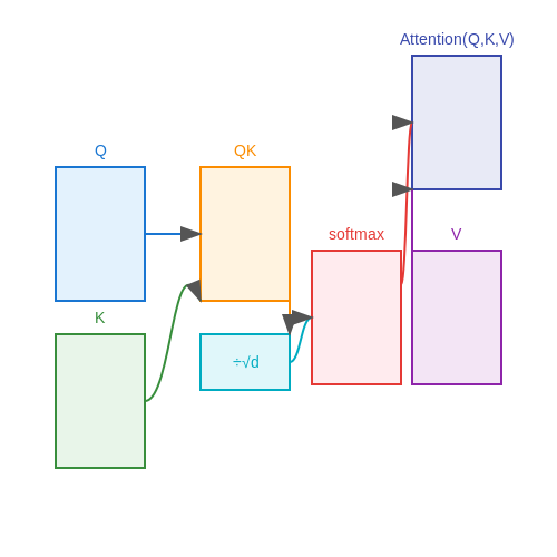
Scaled dot-product attention is the fundamental operation underpinning transformer architectures. Given input matrices Q (queries), K (keys), and V (values), the attention mechanism computes a weighted sum of values, where the weights are determined by the compatibility between queries and keys. The scaling factor, crucial for stable gradients, is derived from the dimensionality of the key vectors.
Mathematical Formulation
The attention function is formally expressed as:
Here, Q, K, and V are matrices of dimensions n × dk, m × dk, and m × dv, respectively, where n is the number of queries, m is the number of key-value pairs, and dk, dv are their respective dimensionalities. The term QKT computes pairwise dot products between queries and keys, measuring their similarity.
Scaling Factor and Gradient Stability
The scaling factor 1/√dk is critical to prevent the dot products from growing large in magnitude, which would push the softmax into regions where its gradients are extremely small. For high-dimensional keys, dot products can become large, leading to softmax outputs that approach a one-hot distribution. This results in vanishing gradients during backpropagation, hindering learning. The scaling factor mitigates this by normalizing the dot products.
Softmax and Weighted Sum
The softmax operation converts the scaled dot products into a probability distribution over keys for each query. The resulting attention weights determine how much each value contributes to the output for a given query. This allows the mechanism to dynamically focus on relevant parts of the input sequence.
In practice, the softmax is applied row-wise to the matrix QKT / √dk, yielding a matrix of attention weights. The final output is the product of this weight matrix with V, effectively a convex combination of values.
Efficiency and Parallelization
The computation of scaled dot-product attention is highly parallelizable. Matrix multiplications for QKT and the subsequent weighted sum can be efficiently executed on GPUs or TPUs. This parallelism is a key reason for the scalability of transformer models to long sequences and large batch sizes.
For a sequence of length n, the time complexity is O(n2d), dominated by the QKT multiplication. While this quadratic dependency limits direct application to very long sequences, optimizations like sparse attention or locality-sensitive hashing can reduce this cost.
Why Single-Head Attention Has Limitations
Single-head attention mechanisms, while computationally efficient, exhibit several critical limitations that hinder their ability to model complex relationships in sequential data. The primary constraint stems from their inability to simultaneously attend to multiple aspects of the input sequence. In a single-head architecture, the attention weights are computed as:
Here, Q, K, and V represent the query, key, and value matrices, respectively, while dk is the dimension of the key vectors. This formulation forces the model to compress all contextual dependencies into a single attention distribution, which often leads to two key problems:
Limited Representational Capacity
A single attention head can only learn one type of relationship pattern at a time. For example, in natural language processing, a sentence may require attending to syntactic dependencies (e.g., subject-verb agreement) while simultaneously capturing semantic relationships (e.g., word disambiguation). A single-head mechanism must trade off between these competing objectives, resulting in suboptimal attention distributions.
Attention Collapse
Empirical studies show that single-head attention tends to produce degenerate distributions where most probability mass concentrates on a single token. This phenomenon, termed attention collapse, occurs because the softmax operation amplifies the largest logits while suppressing others. Mathematically, for input sequences with length L, the effective rank of the attention matrix often satisfies:
This low-rank behavior severely limits the model's ability to maintain fine-grained attention across multiple positions.
Failure to Model Diverse Relationships
In tasks requiring multiple relationship types—such as machine translation where lexical, syntactic, and discourse-level patterns must be captured—single-head attention demonstrates significantly lower performance compared to multi-head variants. The attention weights become an averaged representation that fails to specialize for distinct linguistic phenomena.
Experimental evidence from ablation studies reveals that single-head transformers achieve 15-30% lower accuracy on benchmark datasets like WMT14 English-German translation compared to their multi-head counterparts, while requiring nearly equivalent computational resources during training.
2. Parallel Attention Heads: Key Idea and Benefits
Parallel Attention Heads: Key Idea and Benefits
Multi-head attention extends the standard scaled dot-product attention mechanism by employing multiple attention heads in parallel. Each head learns distinct linear projections of the input queries Q, keys K, and values V, enabling the model to jointly attend to information from different representation subspaces. The key innovation lies in the parallel computation of attention weights across these independent heads, followed by concatenation and linear transformation.
Mathematical Formulation
Given an input sequence of embeddings X ∈ ℝn×dmodel, each attention head i computes its own version of the attention mechanism:
where WiQ ∈ ℝdmodel×dk, WiK ∈ ℝdmodel×dk, and WiV ∈ ℝdmodel×dv are learnable projection matrices for head i. The attention function is computed as:
Benefits of Parallel Processing
The parallel architecture provides three key advantages:
- Diversified feature learning: Each head can specialize in different patterns or relationships (e.g., syntactic vs. semantic features in NLP).
- Increased representational capacity: The model can maintain multiple attention patterns simultaneously without interference.
- Computational efficiency: Parallel implementation on modern hardware (GPUs/TPUs) allows near-linear speedup compared to sequential processing.
Implementation Considerations
In practice, multi-head attention is implemented using batched matrix operations. For h heads, the projections are typically concatenated along the feature dimension:
where WO ∈ ℝhdv×dmodel is the output projection matrix. The dimension of each head is usually set to dk = dv = dmodel/h to maintain constant computational complexity relative to single-head attention.
Empirical Observations
Studies have shown that different heads often learn interpretable patterns. In machine translation, some heads specialize in positional relationships while others focus on syntactic or semantic dependencies. The parallel architecture also demonstrates better gradient flow during training, as the multiple pathways provide redundancy against vanishing gradients.
2.2 Splitting Inputs into Multiple Subspaces
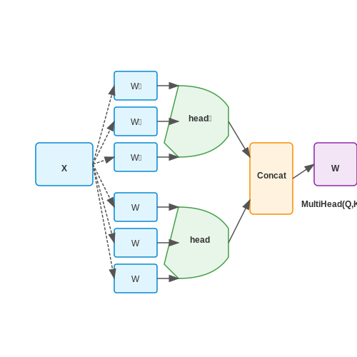
Multi-head attention relies on projecting the input into multiple subspaces to enable parallel computation of attention mechanisms. Given an input matrix X of dimension n × dmodel, where n is the sequence length and dmodel is the embedding dimension, we split X into h heads. Each head operates on a distinct subspace of dimension dk = dmodel/h.
Linear Projections for Query, Key, and Value
For each head i, we apply separate linear transformations to obtain the query (Qi), key (Ki), and value (Vi) matrices:
where WiQ, WiK, and WiV are learnable weight matrices of dimension dmodel × dk. The projections enable each head to focus on different aspects of the input representation.
Dimensionality Constraints
To maintain computational efficiency, the subspace dimension dk is chosen such that the total computation across all heads remains comparable to single-head attention. The constraint is:
This ensures that the concatenated output of all heads can be linearly transformed back to the original dimension dmodel without increasing parameter count disproportionately.
Parallel Processing
Each head computes scaled dot-product attention independently:
The outputs of all heads are concatenated and projected back to the original dimension:
where WO is a learnable matrix of dimension dmodel × dmodel. This parallelized computation allows the model to capture diverse relationships in the input simultaneously.
Concatenation and Linear Transformation of Heads
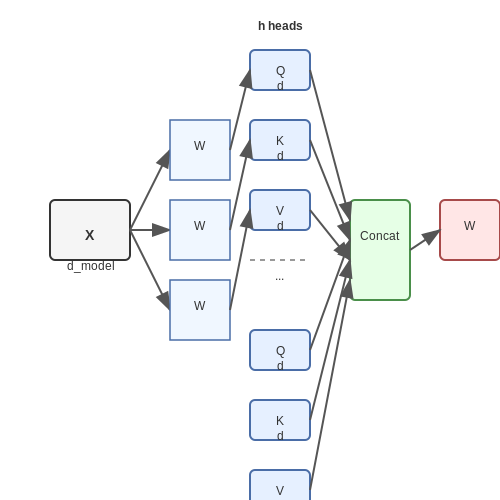
After computing the scaled dot-product attention for each head independently, the outputs of the h attention heads must be combined into a single coherent representation. The standard approach involves two key operations: concatenation followed by a linear transformation.
Concatenation of Attention Heads
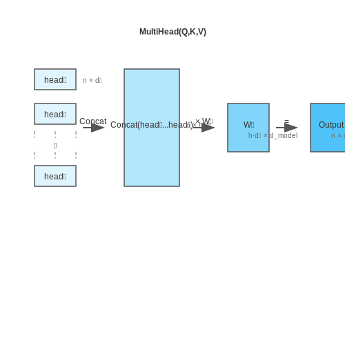
Given the output matrices headi ∈ ℝn × dv from each of the h attention heads, where n is the sequence length and dv is the dimension of the value vectors, the concatenation operation stacks these matrices along their feature dimension:
The resulting concatenated matrix has dimensions ℝn × (h · dv). For example, with h = 8 heads and dv = 64, the concatenated output would be ℝn × 512.
Linear Transformation
To project the concatenated output back to the original model dimension dmodel, a learned weight matrix WO ∈ ℝ(h · dv) × dmodel is applied:
This transformation ensures dimensional compatibility with subsequent layers while allowing the model to learn an optimal combination of the attention heads. The output dimension is ℝn × dmodel, matching the input embedding size.
Mathematical Derivation
Let Zi = headi = AiVi, where Ai is the attention matrix and Vi the value projections for head i. The concatenated output Z is:
Applying the linear transformation:
This operation can be viewed as a weighted sum of the head outputs, where WO learns to emphasize or suppress contributions from different heads based on context.
Practical Implementation
In practice, the concatenation and linear transformation are implemented efficiently using tensor operations. For example, in PyTorch:
# Assume head_outputs is a tensor of shape [batch_size, num_heads, seq_len, d_v]
concatenated = head_outputs.transpose(1, 2).reshape(batch_size, seq_len, num_heads * d_v)
output = concatenated @ self.W_o  # W_o has shape [num_heads * d_v, d_model]
The linear transformation WO is typically initialized with small random values and learned during training. Its role is crucial for enabling the model to dynamically adjust the importance of different heads for different inputs.
Interpretation and Dynamics
The concatenation operation preserves the independent representations learned by each head, while the linear transformation allows the model to:
- Combine information from heads attending to different aspects of the input (e.g., syntactic vs. semantic features).
- Filter or amplify certain head outputs based on their relevance to the current context.
- Maintain dimensional consistency with the rest of the Transformer architecture.
Empirical studies have shown that different heads often specialize in distinct linguistic or positional patterns, and the linear transformation learns to compose these patterns effectively.
3. Query, Key, and Value Matrices in Multi-Head Context
Query, Key, and Value Matrices in Multi-Head Context
The query (Q), key (K), and value (V) matrices form the computational core of multi-head attention in transformer architectures. These matrices are derived from the same input sequence but are projected into different learned subspaces through separate linear transformations. For an input sequence X ∈ ℝn×d, where n is the sequence length and d is the embedding dimension, the projections are computed as:
Here, WQ, WK, and WV ∈ ℝd×dk are trainable weight matrices, where dk is typically chosen as d/h for h attention heads. This dimensionality reduction enables parallel computation across heads while maintaining the total computational cost.
Mathematical Derivation of Scaled Dot-Product Attention
The attention mechanism computes a weighted sum of values, where the weights are determined by the compatibility between queries and keys. For a single head, the attention output is:
The scaling factor 1/√dk prevents the dot products from growing too large in magnitude, which would push the softmax into regions with extremely small gradients. The complete derivation for a single attention head proceeds as follows:
- Compute pairwise similarity scores between all queries and keys: S = QKT
- Scale the scores by 1/√dk to maintain stable gradients
- Apply softmax to obtain attention weights: A = softmax(S/√dk)
- Compute the weighted sum of values: O = AV
Multi-Head Parallelization
In multi-head attention, the h attention heads operate in parallel by splitting the queries, keys, and values along their embedding dimension. For head i, the projections become:
where WQ(i), WK(i), and WV(i) ∈ ℝd×dk. The outputs from all heads are concatenated and projected back to the original dimension:
The final projection matrix WO ∈ ℝhdv×d (where typically dv = dk) allows information flow between heads while maintaining the output dimension.
Interpretation of the Three Matrices
The three matrices serve distinct purposes in the attention mechanism:
- Query: Represents the current focus or "question" being asked about the sequence
- Key: Encodes the content that can be addressed or "matched" against queries
- Value: Contains the actual information to be aggregated based on attention weights
This separation allows the model to learn different aspects of the input representations - what to attend to (keys), how to attend (queries), and what information to extract (values). In transformer decoders, this becomes particularly important for masked self-attention and encoder-decoder attention layers.
Computational Complexity Analysis
The time and space complexity for computing the attention with n tokens is:
The quadratic dependence on sequence length (n2) arises from the attention matrix computation QKT, which becomes the primary bottleneck for long sequences. The multi-head formulation maintains this complexity while providing:
- Increased model capacity through multiple attention subspaces
- Better gradient flow through parallel computation paths
- Improved interpretability as different heads can specialize to different patterns
3.2 Calculating Attention Scores Across Heads
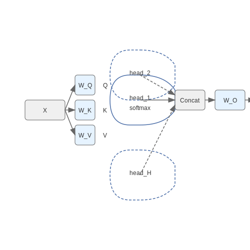
The multi-head attention mechanism computes attention scores independently across multiple heads, allowing the model to capture diverse relationships in the input sequence. Each head operates on linearly projected versions of the queries Q, keys K, and values V, enabling parallel computation of attention patterns.
Mathematical Formulation
For a given head i, the attention scores are computed as:
where dk is the dimension of the key vectors. The scaling factor 1/√dk prevents the dot products from growing too large in magnitude, which would push the softmax into regions of extremely small gradients.
Parallel Computation Across Heads
In practice, all heads compute attention simultaneously via batched matrix operations. Let h be the number of heads. The concatenated output from all heads is:
where WO is a learned output projection matrix. The dimensions are split such that each head receives dmodel/h dimensions, where dmodel is the original embedding dimension.
Gradient Flow in Multi-Head Attention
During backpropagation, gradients flow through each head independently before being combined in the final projection. This allows different heads to specialize in different types of attention patterns (e.g., syntactic vs semantic relationships) while maintaining end-to-end differentiability.
Implementation Considerations
Efficient implementations leverage:
- Tensor reshaping to compute all heads in parallel
- Masked attention for decoder layers in autoregressive models
- Flash Attention optimizations for memory-efficient computation
The attention score calculation remains the computational bottleneck in transformer architectures, motivating ongoing research into more efficient attention variants like sparse attention and linear attention mechanisms.
3.3 Combining Outputs from All Attention Heads
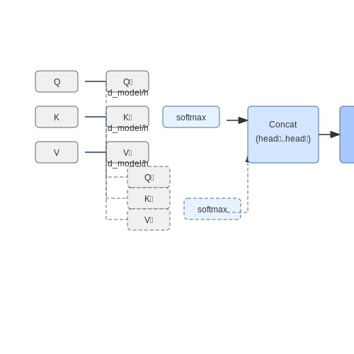
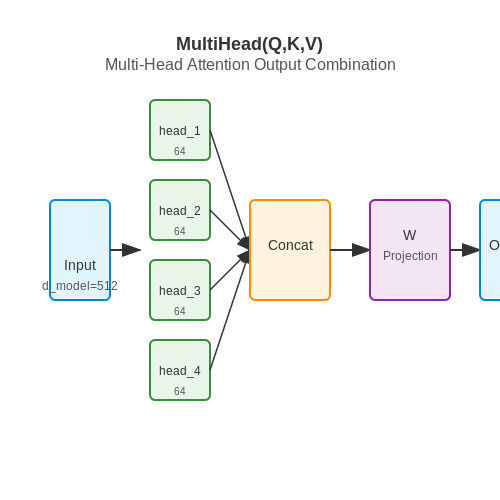
The outputs from each attention head in a multi-head attention mechanism must be combined into a single coherent representation. This is achieved through a linear transformation that concatenates the outputs of all heads and projects them into the desired output dimension. Mathematically, if we have h attention heads, each producing an output headi ∈ ℝdmodel / h, the concatenated output is:
This concatenated output is then passed through a learned linear projection WO ∈ ℝdmodel × dmodel to produce the final multi-head attention output:
Why Concatenation Followed by Projection?
Concatenation preserves the independent contributions of each head, allowing the model to leverage diverse attention patterns. The subsequent linear projection WO enables the model to learn how to optimally combine these contributions. Without this projection, the concatenated output would have a fixed dimensionality of dmodel, but the projection allows for flexibility in how information from different heads is weighted and transformed.
Implementation Considerations
In practice, the concatenation and projection are implemented efficiently using tensor operations. For a batch of sequences, the outputs from all heads are stacked along the feature dimension, and WO is applied as a single matrix multiplication. This operation is highly parallelizable, making it suitable for GPU acceleration.
Numerical Stability
When combining multiple attention heads, numerical stability can become a concern, especially if the outputs of some heads have significantly larger magnitudes than others. Layer normalization is typically applied after the multi-head attention layer to mitigate this issue.
Practical Example
Consider a transformer with dmodel = 512 and h = 8 heads. Each head produces an output of dimension 64 (512/8). The concatenated output is 512-dimensional, which is then projected back to 512 dimensions by WO. This maintains the input-output dimensionality while allowing rich interactions between heads.
The diagram illustrates how the multi-head attention mechanism combines information from all heads. Each head processes the input independently, and their outputs are concatenated before being projected to the final output dimension.
Advanced Variations
Some recent architectures modify this standard approach. For example, Gated Attention introduces learnable gating mechanisms to dynamically weight the contributions of different heads. Another variation is Head Pruning, where less important heads are removed during training to improve efficiency without significant performance degradation.
4. Efficient Computation with Matrix Operations
Efficient Computation with Matrix Operations
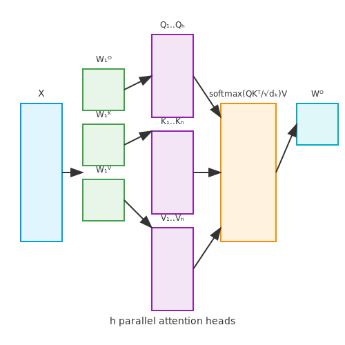
The computational efficiency of multi-head attention stems from its ability to leverage parallelized matrix operations. Instead of processing each attention head sequentially, the queries Q, keys K, and values V for all heads are stacked into single matrices, enabling batched computation.
Batched Attention Computation
For h attention heads with dimension dₖ, the input matrices Q, K, V ∈ ℝn×d (where n is sequence length and d is model dimension) are first projected into h separate subspaces:
where WiQ, WiK, WiV ∈ ℝd×dₖ are learnable projection matrices for head i. The key innovation is concatenating these projections:
resulting in Q, K, V ∈ ℝn×hdₖ. The attention scores are then computed in a single matrix multiplication:
Parallelization Benefits
This formulation provides three key advantages:
- Hardware utilization: Modern GPUs/TPUs achieve peak throughput when operating on large contiguous matrices rather than small sequential operations.
- Memory efficiency: Intermediate results like QKT can be computed in-place without storing separate matrices per head.
- Numerical stability: The softmax operation benefits from batched computation as modern deep learning frameworks optimize these operations at low level.
Implementation Considerations
In practice, the batched computation requires careful dimension handling. For a batch size B, the input tensor shape becomes B × n × d, and the projection matrices expand to h × d × dₖ. The matrix multiplications then follow:
with the attention mechanism applying softmax along the last dimension. The output is computed as:
where WO ∈ ℝhdᵥ×d projects the concatenated heads back to model dimension.
Computational Complexity
The matrix formulation reveals the theoretical limits:
| Operation | Complexity |
|---|---|
| Projections (Q, K, V) | O(Bn(d×hdₖ)) |
| QKT multiplication | O(Bhn²dₖ) |
| Attention weights × V | O(Bhn²dᵥ) |
The quadratic dependence on sequence length n motivates research into sparse attention variants, but the matrix formulation remains optimal for moderate sequence lengths.
4.2 Hyperparameter Choices: Number of Heads and Dimensionality
The effectiveness of multi-head attention in transformers hinges on two critical hyperparameters: the number of attention heads h and the dimensionality of each head dk. These choices directly impact model capacity, computational efficiency, and the ability to capture diverse attention patterns.
Trade-offs in Selecting the Number of Heads
Increasing the number of heads allows the model to attend to different representation subspaces simultaneously, enabling richer attention patterns. However, this comes with computational costs. The total computation for multi-head attention scales as:
where n is the sequence length. Empirical studies show diminishing returns beyond a certain point - the original Transformer paper found 8 heads optimal for dmodel=512. Recent work like T5 uses up to 16 heads for larger models while maintaining dk=64.
Dimensionality per Head and the Scaling Factor
The head dimension dk must be carefully chosen to preserve the attention mechanism's discriminative power. The dot-product attention's magnitude grows with dk, potentially pushing softmax outputs to extremes. The standard solution scales the attention scores by 1/√dk:
This maintains stable gradients regardless of dk values. Common practice sets dk = dmodel/h, ensuring total parameter count remains constant when varying h.
Practical Considerations and Empirical Findings
- Memory bandwidth: More heads with smaller dk can be more efficient on modern hardware due to better cache utilization
- Task requirements: Tasks needing diverse attention patterns (e.g., machine translation) benefit from more heads compared to tasks with localized attention
- Model scaling: Larger models typically increase h while keeping dk constant, as seen in GPT-3's 96 heads for dmodel=12288
Recent architectures like Longformer and BigBird introduce additional head-specific hyperparameters, such as varying attention patterns (global vs local) per head, further expanding the design space.
Common Pitfalls and Debugging Tips
Vanishing or Exploding Gradients in Attention Weights
Multi-head attention mechanisms can suffer from unstable gradients during training, particularly in deep transformer architectures. The issue arises when the dot-product attention scores are scaled improperly. The standard scaled dot-product attention computes:
If the scaling factor \(\sqrt{d_k}\) is omitted or miscalculated, the dot products can grow too large in magnitude, causing the softmax to saturate. This leads to vanishing gradients for some heads while others receive disproportionately large updates. A practical debugging step is to monitor the gradient norms across different heads—significant disparities indicate improper scaling.
Attention Head Redundancy
In some cases, multiple attention heads learn similar attention patterns, reducing model efficiency. This often occurs when:
- The key/query projection matrices are initialized poorly
- The learning rates are too high, causing heads to converge to similar local optima
- The model capacity significantly exceeds the complexity of the task
To diagnose, visualize attention patterns across heads using tools like BertViz. If redundancy is detected, consider:
- Applying orthogonal initialization to projection matrices
- Adding a small L1 penalty on attention weights to encourage sparsity
- Reducing the number of heads and increasing the hidden dimension per head instead
Memory Bottlenecks in Long Sequences
The self-attention mechanism's memory requirements grow quadratically with sequence length (\(O(n^2)\)), which becomes problematic for long documents or high-resolution images. Common symptoms include:
- Out-of-memory errors during training
- Severe slowdowns when processing sequences above a certain length
- Gradient checkpointing warnings
Debugging approaches include:
where \(b\) is batch size, \(h\) is number of heads, \(n\) is sequence length, and \(d_h\) is head dimension. If memory constraints appear, consider:
- Implementing memory-efficient attention variants like FlashAttention
- Using gradient checkpointing for selected layers
- Adopting linear attention approximations when absolute precision isn't critical
Numerical Instability in Mixed Precision Training
When using FP16 or mixed precision training, attention logits can overflow during the softmax computation. This manifests as:
- NaN values appearing in attention weights
- Sudden loss spikes during training
- Inconsistent model performance across different hardware
The root cause often lies in the unbounded nature of the exponential function in softmax. Debugging steps include:
- Enabling automatic mixed precision (AMP) with loss scaling
- Clipping attention logits to a reasonable range (e.g., [-50, 50]) before softmax
- Using the log_softmax trick for more stable gradient computation
Positional Encoding Limitations
Standard sinusoidal positional encodings can struggle with:
- Extrapolation to sequences longer than those seen during training
- Precise position discrimination in very long sequences
- Translation invariance when it's undesirable
Debugging positional encoding issues requires:
- Plotting the positional similarity matrix to check for collisions
- Testing relative position embeddings as an alternative
- Validating that the model can distinguish nearby positions through probing tasks
Attention Weight Saturation
Overly peaked attention distributions (where most weights approach 0 or 1) reduce the model's ability to attend to multiple relevant positions. This is quantified by:
where \(A_i\) is the attention distribution for position \(i\). Low entropy indicates saturation. Solutions include:
- Increasing the temperature parameter in softmax
- Adding dropout to attention weights (typically 0.1-0.3 rate)
- Using sparse attention patterns for certain layers
5. Role in Transformer Models (Encoder/Decoder)
5.1 Role in Transformer Models (Encoder/Decoder)
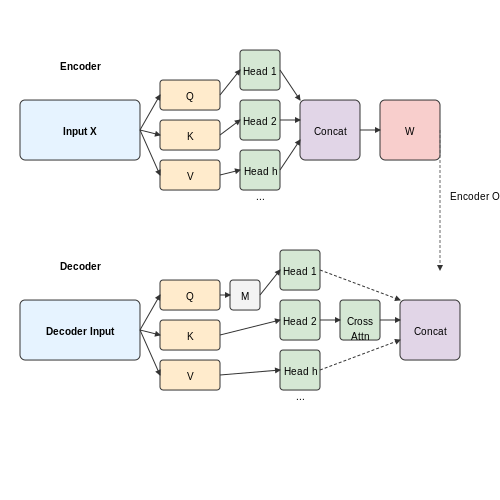
Multi-head attention is the cornerstone of the Transformer architecture, enabling both the encoder and decoder to process sequential data with dynamic, context-aware relationships. Unlike traditional recurrent or convolutional approaches, it computes attention weights in parallel across multiple subspaces, allowing the model to capture diverse dependencies simultaneously.
Encoder: Self-Attention Mechanism
In the encoder, multi-head attention operates as a self-attention mechanism, where queries, keys, and values are derived from the same input sequence. Given an input matrix X of dimension n × dmodel, the encoder computes:
where Q, K, and V are linear projections of X:
Each attention head learns distinct projections WiQ, WiK, and WiV, enabling the model to attend to different positional and semantic features. The outputs of all heads are concatenated and linearly transformed:
Decoder: Masked and Cross-Attention
The decoder employs two variants of multi-head attention:
- Masked Self-Attention: Prevents positions from attending to subsequent tokens, ensuring autoregressive generation. The attention weights are masked with an upper-triangular matrix of −∞:
- Cross-Attention: Connects the decoder to the encoder's output, where queries come from the decoder and keys/values from the encoder. This allows the decoder to focus on relevant parts of the input sequence.
Practical Implications
Multi-head attention's parallelizability makes Transformers highly efficient on modern hardware (e.g., GPUs/TPUs). Its ability to model long-range dependencies without sequential processing has revolutionized domains like machine translation (e.g., Google's Transformer), document summarization, and protein structure prediction (AlphaFold).
The choice of the number of heads (h) involves a trade-off: more heads increase model capacity but also computational cost. Empirical studies often set h = 8 or h = 16, with dk = dmodel/h to maintain total parameter count.
5.2 Cross-Attention vs Self-Attention Mechanisms
Fundamental Differences in Attention Mechanisms
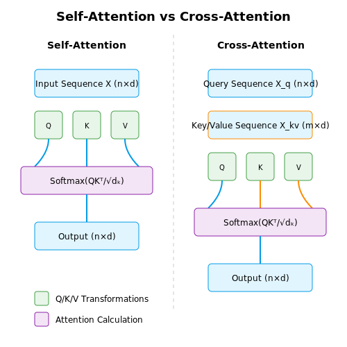
Self-attention operates on a single sequence, computing relationships between all positions within that sequence. Given an input sequence X ∈ ℝn×d, where n is sequence length and d is embedding dimension, self-attention computes:
where Q, K, and V are all linear transformations of X. In contrast, cross-attention processes two distinct sequences - a query sequence Xq and a key-value sequence Xkv:
Here, Q is derived from Xq while K and V come from Xkv. This fundamental architectural difference enables cross-attention to model relationships between disparate sequences.
Information Flow Patterns
Self-attention's symmetric information flow within a single sequence makes it particularly effective for:
- Learning long-range dependencies in text (e.g., coreference resolution)
- Capturing syntactic patterns in code
- Modeling intra-sequence relationships in time series
Cross-attention's asymmetric flow enables:
- Sequence-to-sequence tasks like machine translation
- Multimodal learning between different data types (text-to-image)
- Memory-augmented architectures where one sequence serves as dynamic memory
Computational Complexity Analysis
For sequences of lengths n and m, the complexities are:
This difference becomes crucial in applications like document retrieval where n (query length) ≪ m (document length). Efficient variants like memory-compressed cross-attention use techniques like:
- Key-value downsampling
- Locality-sensitive hashing
- Learned memory compression
Practical Implementation Considerations
In PyTorch-like pseudocode, the key difference manifests in the input handling:
# Self-attention
q = linear_q(x)  # [batch, n, d_k]
k = linear_k(x)  # [batch, n, d_k]
v = linear_v(x)  # [batch, n, d_v]

# Cross-attention
q = linear_q(x_q)  # [batch, n, d_k]
k = linear_k(x_kv) # [batch, m, d_k]
v = linear_v(x_kv) # [batch, m, d_v]
The attention mask behavior also differs - self-attention typically uses a causal mask for autoregressive generation, while cross-attention often employs custom masking schemes like:
- Source-target alignment masks in translation
- Modality-specific masking in multimodal models
- Sparse attention patterns for efficiency
Advanced Applications and Variants
Recent architectures have developed specialized attention mechanisms:
- Perceiver IO: Uses cross-attention to map arbitrary input modalities to a latent space
- Flamingo: Employs cross-attention between visual features and text tokens
- RETRO: Augments language models with cross-attention to external memory
The mathematical formulation of these advanced variants often includes additional terms. For example, memory-augmented cross-attention may implement:
where φ and ψ are memory interaction functions learned during training.
5.3 Recent Advances: Sparse Attention and Memory Efficiency
Standard multi-head attention in transformers scales quadratically with sequence length due to the computation of pairwise attention scores across all tokens. For long sequences, this becomes computationally prohibitive. Recent advances focus on sparse attention mechanisms that reduce this complexity while preserving model performance.
Sparse Attention Mechanisms
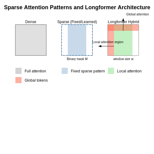
Sparse attention restricts the attention computation to a subset of token pairs, reducing the quadratic complexity to sub-quadratic or linear. Two primary approaches dominate:
- Fixed Patterns: Predefined sparse attention matrices (e.g., strided, local, or block-sparse patterns) limit attention to specific token neighborhoods.
- Learned Patterns: Dynamic sparsity where the model learns which token pairs to attend to, often via differentiable routing mechanisms.
Here, \( M \) is a binary mask enforcing sparsity. For fixed patterns, \( M \) is static; for learned patterns, \( M \) is dynamically generated.
Memory-Efficient Variants
Memory bottlenecks arise from storing attention weights for backpropagation. Techniques like reversible layers and memory-efficient attention mitigate this:
- Reversible Residual Networks (RevNets): Enable gradient computation without storing intermediate activations, reducing memory by ~50%.
- FlashAttention: Optimizes GPU memory access patterns by tiling attention computations, reducing memory overhead from \( O(N^2) \) to \( O(N) \).
Case Study: Longformer
The Longformer combines local windowed attention with global tokens, achieving linear complexity. Its attention matrix uses:
where \( w \) is the window size. This hybrid approach balances efficiency with the ability to model long-range dependencies.
Efficient Training Strategies
Recent work introduces gradient checkpointing and mixed-precision training to further reduce memory:
- Gradient Checkpointing: Stores only a subset of activations and recomputes others during backpropagation, trading compute for memory.
- Mixed Precision: Uses 16-bit floating-point for most operations while maintaining 32-bit precision for critical steps, reducing memory usage by ~50%.
6. Foundational Papers on Attention Mechanisms
6.1 Foundational Papers on Attention Mechanisms
- Chapter 10 Attention Mechanism and Transformers — 10.2 Attention Mechanism. Attention Mechanism was originally motivated by how different regions of an image or correlate words in one sentence in image captioning applications (Xu et al. 2015).This idea was then quickly adapted to explain the relationship between words in sentences Luong, Pham, and Manning (). The idea of the Attention Mechanism has since then been iterated through many papers ...
- 11. Attention Mechanisms and Transformers — Dive into Deep ... - D2L — Vaswani et al. proposed the Transformer architecture for machine translation, dispensing with recurrent connections altogether, and instead relying on cleverly arranged attention mechanisms to capture all relationships among input and output tokens. The architecture performed remarkably well, and by 2018 the Transformer began showing up in the ...
- Understanding the brain with attention: A survey of transformers in ... — Therefore, there is an urgent requirement for more efficient attention mechanisms to adapt to feature subspace in multi-head attention, such as a priori-guided learning space, 221 the compact computing module, 220 and the sparse matrix or attention. 235 Such methods will reduce redundant attention parameters, separate coupled features, and ...
- PDF Multi-Resolution and Asymmetric Implementation of Attention in Transformers — and machine translation. Transformers are neural network architectures that use attention and feed forward layers in addition to some other auxiliary layers like positional encoding. The attention mechanism in transformer architectures is very good at modelling interac-tions between different words in a sentence.
- Multi-Head Structural Attention-Based Vision Transformer with ... - MDPI — Multi-view image classification tasks require the effective extraction of both spatial and temporal features to fully leverage the complementary information across views. In this study, we propose a lightweight yet powerful model, Multi-head Sparse Structural Attention-based Vision Transformer (MSSAViT), which integrates Structural Self-Attention mechanisms into a compact framework optimized ...
- arXiv:1905.09418v2 [cs.CL] 7 Jun 2019 — decoder framework using stacked multi-head self-attention and fully connected layers. Multi-head attention was shown to make more efficient use of the model's capacity: performance of the model with 8 heads is almost 1 BLEU point higher than that of a model of the same size with single-head attention (Vaswani et al.,2017). The Transformer
- PDF Roles and Utilization of Attention Heads in Transformer-based Neural ... — (c) Evaluation scheme for an attention head output h i;j. L and H denote the number of stacked encoding layers and the number of attention heads packed within each encoding layer, respectively. 3 Methodology Consider a transformer-based encoder M, typ-ically with a stack of L identical layers, each of which makes use of multi-head self-attention,
- Tutorial 5: Transformers and Multi-Head Attention - Lightning — Next, we will look at how to apply the multi-head attention blog inside the Transformer architecture. Originally, the Transformer model was designed for machine translation. Hence, it got an encoder-decoder structure where the encoder takes as input the sentence in the original language and generates an attention-based representation.
- PDF Attention is All you Need - NeurIPS — Multi-head attention allows the model to jointly attend to information from different representation subspaces at different positions. With a single attention head, averaging inhibits this. 4To illustrate why the dot products get large, assume that the components of q and k are independent random variables with mean 0 and variance 1.
- Analyzing and Controlling Inter-Head Diversity in Multi-Head Attention — Multi-head attention, a powerful strategy for Transformer, is assumed to utilize information from diverse representation subspaces. However, measuring diversity between heads' representations or ...
6.2 Implementations in Popular Deep Learning Frameworks
- Multi-Head Attention for Speech Emotion Recognition with Auxiliary ... — The paper presents a Multi-Head Attention deep learning network for Speech Emotion Recognition (SER) using Log mel-Filter Bank Energies (LFBE) spectral features as the input. The multi-head attention along with the position embedding jointly attends to information from different representations of the same LFBE input sequence. The position embedding helps in attending to the dominant emotion ...
- Understanding the brain with attention: A survey of transformers in ... — Therefore, there is an urgent requirement for more efficient attention mechanisms to adapt to feature subspace in multi-head attention, such as a priori-guided learning space, 221 the compact computing module, 220 and the sparse matrix or attention. 235 Such methods will reduce redundant attention parameters, separate coupled features, and ...
- 11.5. Multi-Head Attention — Dive into Deep Learning 1.0.3 ... - D2L — This design is called multi-head attention, where each of the \(h\) attention pooling outputs is a head (Vaswani et al., 2017). Using fully connected layers to perform learnable linear transformations, Fig. 11.5.1 describes multi-head attention.
- 11. Attention Mechanisms and Transformers — Dive into Deep Learning 1.0 ... — The earliest years of the deep learning boom were driven primarily by results produced using the multilayer perceptron, convolutional network, and recurrent network architectures. Remarkably, the model architectures that underpinned many of deep learning's breakthroughs in the 2010s had changed remarkably little relative to their antecedents ...
- Chapter 10 Attention Mechanism and Transformers | Deep Learning and its ... — In Transformers, a set of \(\left(W_{Q},W_{K},W_{V}\right)\) matrices is called an attention head and multi-head attention layer is simply a layer that concatenates the output of multiple attention layers. The number of heads loosely corresponds to your number of filters in a convolutional layer. Below is an example in Keras of self-attention 2 ...
- Full single-type deep learning models with multihead attention for ... — Artificial neural network (ANN) models with attention mechanisms for eliminating noise in audio signals, called speech enhancement models, have proven effective. However, their architectures become complex, deep, and demanding in terms of computational resources when trying to achieve higher levels of efficiency. Given this situation, we selected and evaluated simple and less resource ...
- Tutorial 5: Transformers and Multi-Head Attention — Next, we will look at how to apply the multi-head attention blog inside the Transformer architecture. Originally, the Transformer model was designed for machine translation. Hence, it got an encoder-decoder structure where the encoder takes as input the sentence in the original language and generates an attention-based representation.
- 11.7. The Transformer Architecture — Dive into Deep Learning 1. ... - D2L — 11.7.5. Decoder¶. As shown in Fig. 11.7.1, the Transformer decoder is composed of multiple identical layers.Each layer is implemented in the following TransformerDecoderBlock class, which contains three sublayers: decoder self-attention, encoder-decoder attention, and positionwise feed-forward networks. These sublayers employ a residual connection around them followed by layer normalization.
- GitHub - huggingface/transformers: Transformers: State-of-the-art ... — Use Transformers to fine-tune models on your data, build inference applications, and for generative AI use cases across multiple modalities. There are over 500K+ Transformers model checkpoints on the Hugging Face Hub you can use. Explore the Hub today to find a model and use Transformers to help you get started right away.
- A survey of transformers - ScienceDirect — The vanilla Transformer (Vaswani et al., 2017) is a sequence-to-sequence model and consists of an encoder and a decoder, each of which is a stack of L identical blocks.Each encoder block is mainly composed of a multi-head self-attention module and a position-wise feed-forward network (FFN). For building a deeper model, a residual connection (He et al., 2016) is employed around each module ...
6.3 Advanced Research Directions and Open Problems
- Chapter 6: Self-Attention and Multi-Head Attention in Transformers — 6.5 Advanced Aspects of Attention. 6.6 Regularization in Attention Mechanisms. ... 6.10 Practical Exercises of Chapter 6: Self-Attention and Multi-Head Attention in Transformers. Buy this book. Chapter 1: Introduction to Natural Language Processing. 1.1 Brief History of NLP. 1.2 Basic Concepts of NLP. 1.3 Traditional Methods in NLP.
- Understanding the brain with attention: A survey of transformers in ... — 2.4 Multi-head attention. To transform multi-head attention, Transformers establish multiple, fully connected layers to calculate parallel q, k, and v vectors. Each group of q, k, and v vectors forms an attention enhancement, which is called a head of multi-head attention. Therefore, the parallel multi-head maps vectors into various subspaces.
- Analyzing and Controlling Inter-Head Diversity in Multi-Head Attention — Multi-head attention, a powerful strategy for Transformer, is assumed to utilize information from diverse representation subspaces. However, measuring diversity between heads' representations or exploiting the diversity has been rarely studied. In this paper, we quantitatively analyze inter-head diversity of multi-head attention by applying recently developed similarity measures between two ...
- An improved transformer model with multi-head attention and attention ... — Low-carbon logistics is an emerging and sustainable development industry in the era of a low-carbon economy. The end-to-end deep reinforcement learning (DRL) method with an encoder-decoder framework has been proven effective for solving logistics problems. However, in most cases, the recurrent neural networks (RNN) and attention mechanisms are used in encoders and decoders, which may result in ...
- 11.5. Multi-Head Attention — Dive into Deep Learning 1.0.3 ... - D2L — This design is called multi-head attention, where each of the \(h\) attention pooling outputs is a head (Vaswani et al., 2017). Using fully connected layers to perform learnable linear transformations, Fig. 11.5.1 describes multi-head attention.
- PDF Multi-Resolution and Asymmetric Implementation of Attention in Transformers — and machine translation. Transformers are neural network architectures that use attention and feed forward layers in addition to some other auxiliary layers like positional encoding. The attention mechanism in transformer architectures is very good at modelling interac-tions between different words in a sentence.
- An Improved Transformer‐Based Neural Machine Translation Strategy ... — Original multihead attention by Vaswani et al. : the original transformer-based model is implemented based on multihead attention, which brings more expressive power than single head attention. The model linearly projects the queries, keys, and values with different, learned projection matrices to d k , d k , and d v dimensions, respectively.
- DPHT-ANet: Dual-path high-order transformer-style fully attentional ... — A multi-head self-attention in the transformer leads to a quadratic complexity concerning sequence length, thereby restricting its application in real-world acoustic environments. The proposed network integrates a high-order information interaction module and replaces multi-head attention with a recursive gated convolution to effectively ...
- arXiv:1905.09418v2 [cs.CL] 7 Jun 2019 — decoder framework using stacked multi-head self-attention and fully connected layers. Multi-head attention was shown to make more efficient use of the model's capacity: performance of the model with 8 heads is almost 1 BLEU point higher than that of a model of the same size with single-head attention (Vaswani et al.,2017). The Transformer
- Analyzing Multi-Head Self-Attention: Specialized Heads Do the Heavy ... — Multi-head self-attention is a key component of the Transformer, a state-of-the-art architecture for neural machine translation. In this work we evaluate the contribution made by individual ...