Multi-Task Learning with Transformers
1. Key Concepts and Definitions
1.1 Key Concepts and Definitions
Multi-Task Learning (MTL)
Multi-Task Learning (MTL) is a machine learning paradigm where a single model is trained to perform multiple related tasks simultaneously. Unlike traditional single-task learning, MTL leverages shared representations across tasks, often improving generalization by exploiting commonalities and differences among tasks. The underlying hypothesis is that inductive bias from related tasks can enhance the model's performance on each individual task.
Here, T denotes the number of tasks, λi is a task-specific weighting coefficient, Li is the loss for task i, and θshared and θi represent shared and task-specific parameters, respectively.
Transformers in MTL
Transformers, originally introduced for sequence-to-sequence tasks, have become a dominant architecture in MTL due to their self-attention mechanism, which dynamically weights input features. The key advantage lies in their ability to capture hierarchical and task-agnostic patterns, making them ideal for shared representation learning. The transformer's multi-head attention allows the model to focus on different aspects of the input for different tasks.
In this equation, Q, K, and V are the query, key, and value matrices, and dk is the dimension of the key vectors. The scaled dot-product attention enables the model to weigh the importance of different input tokens dynamically.
Task-Specific Adaptations
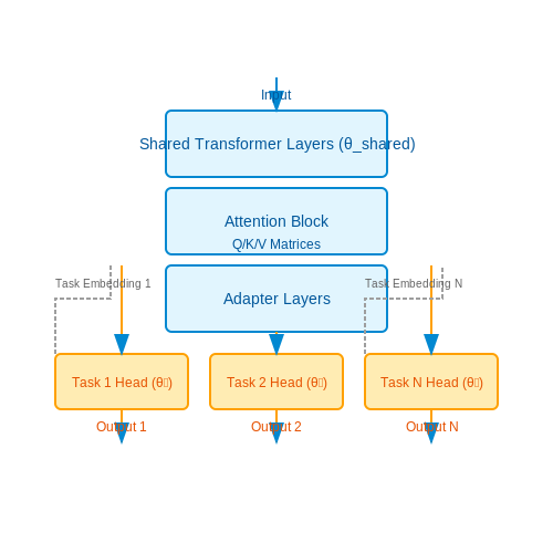
In MTL with transformers, task-specific adaptations are often implemented via:
- Task Embeddings: Learned embeddings that condition the transformer's behavior on the current task.
- Adapter Layers: Lightweight, task-specific modules inserted between transformer layers.
- Multi-Task Heads: Separate output heads for each task, sharing the same backbone.
Challenges in MTL with Transformers
Despite their advantages, MTL with transformers presents several challenges:
- Negative Transfer: Poorly related tasks can degrade performance due to conflicting gradients.
- Task Imbalance: Tasks with varying difficulties or scales may dominate the learning process.
- Scalability: Adding more tasks increases model complexity and computational cost.
Practical Applications
MTL with transformers has been successfully applied in:
- Natural Language Processing: Jointly performing named entity recognition, part-of-speech tagging, and sentiment analysis.
- Computer Vision: Simultaneous object detection, segmentation, and classification.
- Healthcare: Predicting multiple medical outcomes from patient records.
Benefits and Challenges of Multi-Task Learning
Benefits of Multi-Task Learning
Multi-task learning (MTL) with transformers offers several advantages over single-task learning, particularly in scenarios where tasks share underlying representations or require transferable knowledge. The primary benefits include:
- Improved Generalization: By learning shared representations across tasks, MTL acts as an implicit regularizer, reducing overfitting to any single task. The shared parameters must generalize well to multiple objectives, which often leads to better performance on individual tasks compared to training them independently.
- Data Efficiency: MTL enables knowledge transfer between tasks, allowing models to leverage patterns learned from data-rich tasks to improve performance on data-scarce tasks. This is particularly valuable in domains where labeled data is expensive or limited.
- Computational Efficiency: A single multi-task model requires less computational resources than maintaining separate models for each task, both during training and inference. This is especially relevant for transformer architectures where the bulk of computation occurs in the shared encoder.
- Cross-Task Synergy: Certain tasks naturally complement each other. For example, in natural language processing, part-of-speech tagging and named entity recognition share syntactic features that can be mutually reinforced through joint training.
The effectiveness of MTL can be quantified through the improvement in the generalization bound. For k tasks with shared parameters θs and task-specific parameters θi, the expected risk R across tasks is bounded by:
where n is the number of samples per task. The second term shows how MTL benefits from increased effective sample size through parameter sharing.
Challenges of Multi-Task Learning
Despite its advantages, MTL introduces several complexities that must be carefully managed:
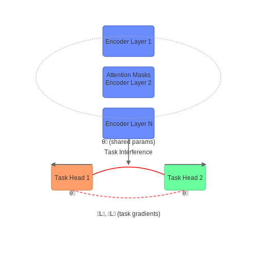
- Task Interference: Negative transfer occurs when optimizing for one task degrades performance on another. This happens when tasks compete for shared parameters or have conflicting gradients. The interference can be measured by the cosine similarity between task gradients:
- Imbalanced Task Difficulty: Tasks with larger gradients or higher loss magnitudes can dominate the optimization process. This is particularly problematic when tasks have different noise levels or learning dynamics.
- Architecture Design: Determining the optimal level of parameter sharing requires careful experimentation. Too much sharing can lead to interference, while too little reduces the benefits of MTL. Transformer architectures typically share lower layers while keeping task-specific heads, but the exact partitioning is non-trivial.
- Optimization Complexity: The loss landscape becomes more complex with multiple objectives. Simple linear combination of task losses often performs suboptimally, requiring dynamic weighting schemes like:
where wi(t) are time-dependent weights that adapt during training.
Practical Considerations
In transformer-based MTL, several architectural choices significantly impact performance:
- Attention Masking: Task-specific attention masks can prevent information leakage between incompatible tasks while still allowing shared computation in lower layers.
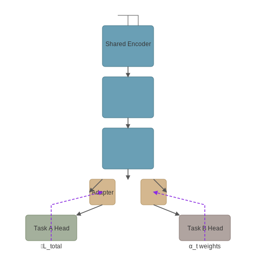
- Adapter Layers: Inserting small task-specific adapter modules between transformer layers maintains most of the parameter sharing while allowing task specialization.
- Gradient Modulation: Techniques like PCGrad project conflicting gradients to avoid interference while preserving beneficial gradient alignment.
The effectiveness of these approaches depends on the task relationships, which can be quantified through the task affinity matrix A ∈ ℝk×k, where Aij measures the performance improvement when tasks i and j are trained together versus separately.
1.3 Architectural Approaches for Multi-Task Learning
Hard Parameter Sharing
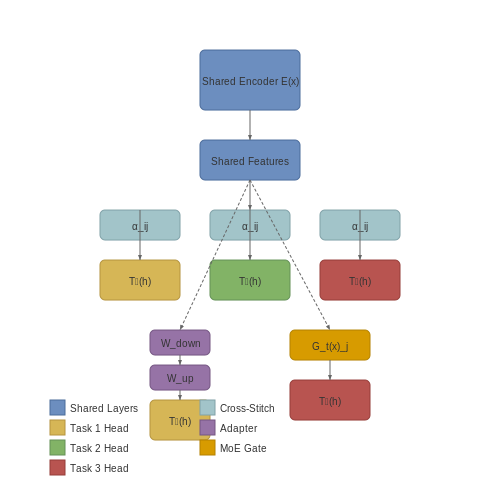
Hard parameter sharing is the most common architectural approach for multi-task learning (MTL) with transformers. In this setup, the model shares all hidden layers across tasks while maintaining task-specific output layers. The shared encoder (e.g., BERT, RoBERTa) processes input data, and task-specific heads branch from the final hidden layer. Mathematically, for N tasks, the shared encoder E produces a representation h = E(x), while task-specific heads Ti compute predictions:
This approach reduces the risk of overfitting, as the shared layers must generalize across all tasks. However, task interference can occur if the objectives conflict, leading to suboptimal performance. Practical implementations often use gradient masking or task-specific learning rates to mitigate this.
Soft Parameter Sharing
Soft parameter sharing allows each task to have its own model parameters while encouraging similarity through regularization. The transformer architecture implements this via:
- Cross-stitch units: Linear combinations of task-specific hidden states.
- Orthogonal regularization: Penalizes dissimilarity between task-specific parameters.
For two tasks with hidden states h1 and h2, a cross-stitch layer computes:
where αij are learnable mixing weights. This provides flexibility but increases computational overhead due to separate parameter sets.
Task-Specific Adapters
Adapter-based architectures insert small task-specific modules between transformer layers while keeping the core model frozen. Each adapter consists of:
- A down-projection to a bottleneck dimension.
- A nonlinear activation (e.g., ReLU).
- An up-projection to the original dimension.
For a hidden state h at layer l, the adapter output is:
where Wdown ∈ ℝd×b and Wup ∈ ℝb×d (b ≪ d). This approach enables parameter-efficient tuning and is widely used in few-shot learning scenarios.
Multi-Gate Mixture-of-Experts
The Mixture-of-Experts (MoE) architecture routes inputs to specialized subnetworks ("experts") via gating mechanisms. In MTL, each task t employs a separate gating network Gt over shared experts {Ej}kj=1:
The gating weights Gt(x) are typically computed via softmax over a learned projection. Sparse gating (e.g., top-2 routing) improves scalability. Google’s Switch Transformer demonstrates this approach at scale, achieving 7x faster inference than dense models.
Gradient Modulation Techniques
Architectures like GradNorm dynamically adjust task-specific gradients during backpropagation. For N tasks with losses {Li}, the modulated gradient for task i is:
where wi(t) is a learned weight updated to balance task learning rates. This is implemented as an additional network head that computes:
with gi = ||\nabla_{W} L_i||2. Such approaches prevent dominant tasks from overwhelming the shared representation.
2. Transformer Architecture Recap
2.1 Transformer Architecture Recap
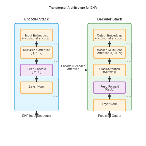
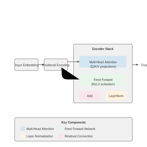
The Transformer architecture, introduced by Vaswani et al. in 2017, revolutionized sequence modeling by replacing recurrent and convolutional layers with self-attention mechanisms. At its core, the Transformer relies on three key components: multi-head attention, position-wise feed-forward networks, and layer normalization. Unlike RNNs, Transformers process entire sequences in parallel, making them highly efficient for modern hardware accelerators.
Self-Attention Mechanism
The self-attention mechanism computes a weighted sum of input representations, where the weights are dynamically derived from pairwise interactions between elements in the sequence. Given an input sequence X ∈ ℝn×d, where n is the sequence length and d is the embedding dimension, the attention operation is defined as:
Here, Q (queries), K (keys), and V (values) are linear projections of the input X:
where WQ, WK, WV ∈ ℝd×dk are learnable weight matrices. The scaling factor 1/√dk prevents gradient saturation in the softmax.
Multi-Head Attention
Multi-head attention extends self-attention by applying h parallel attention heads, each with separate learned projections. This allows the model to jointly attend to information from different representation subspaces:
where each head computes attention independently:
The output projections WO ∈ ℝhdv×d combine the heads' outputs. Typical implementations use h = 8 heads with dk = dv = d/h.
Position-Wise Feed-Forward Networks
Each Transformer layer contains a position-wise feed-forward network (FFN) applied independently to each token representation. The FFN consists of two linear transformations with a ReLU activation in between:
where W1 ∈ ℝd×dff, W2 ∈ ℝdff×d, and dff is typically 4×d. This provides additional nonlinear capacity to the model.
Layer Normalization and Residual Connections
Transformers employ residual connections around each sub-layer (attention and FFN), followed by layer normalization:
This architecture choice enables stable training of deep networks by mitigating vanishing gradients. The layer normalization operates over the embedding dimension d, normalizing activations to zero mean and unit variance for each token independently.
Positional Encoding
Since Transformers lack inherent notion of sequence order, positional encodings are added to input embeddings to inject information about token positions. The original paper uses sinusoidal functions of varying frequencies:
where pos is the position and i is the dimension. Learned positional embeddings are also commonly used in practice.
2.2 Adapting Transformers for Multi-Task Learning
Transformer architectures, originally designed for sequence-to-sequence tasks like machine translation, require careful adaptation to handle multiple tasks simultaneously. The core challenge lies in balancing shared representations across tasks while preserving task-specific nuances. Two primary architectural strategies dominate this space: hard parameter sharing and soft parameter sharing.
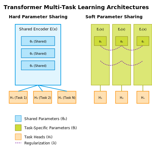
Hard Parameter Sharing
This approach forces all tasks to share most transformer layers, with only the final task-specific heads differing. Mathematically, for N tasks, the shared encoder E processes input x, while task-specific heads Hi produce outputs:
The shared encoder typically comprises the transformer's self-attention and feed-forward layers, enabling cross-task knowledge transfer. A key advantage is reduced computational overhead, as the bulk of parameters are reused. However, task interference can occur when optimization gradients conflict.
Soft Parameter Sharing
More flexible than hard sharing, this method allows separate transformer parameters per task while encouraging similarity through regularization. The loss function often includes a term penalizing divergence between task-specific parameters θi and a shared reference θ0:
Recent variants like Cross-Stitch Networks learn weighted combinations of task-specific features dynamically. The transformer's attention mechanism proves particularly adaptable here—attention heads can specialize in different task relationships while maintaining shared key-value projections.
Architectural Innovations
Several transformer-specific modifications enhance multi-task performance:
- Task Embeddings: Concatenating learned task identifiers to input tokens, enabling the model to conditionally modulate processing.
- Adapter Layers: Inserting small, task-specific modules between transformer layers while keeping core weights frozen.
- Gradient Masking: Selectively backpropagating gradients through shared layers based on task relevance.
The transformer's scalability allows these techniques to compound; for instance, combining adapters with task embeddings often outperforms either method alone. Empirical studies show that lower layers benefit most from hard sharing, while higher layers require more task-specific adaptation.
Optimization Considerations
Training dynamics differ significantly from single-task scenarios. The gradient cosine similarity between tasks predicts compatibility:
Where gi, gj are task gradients. Tasks with positive similarity benefit from joint training, while conflicting gradients may require:
- Gradient Surgery: Projecting conflicting gradients to orthogonal directions
- Dynamic Weighting: Automatically adjusting task loss coefficients based on learning progress
Transformer-specific optimizers like AdaFactor often outperform Adam in multi-task settings due to better memory efficiency and stabler gradient norms across tasks.
Shared vs. Task-Specific Parameters in Transformers
Multi-task learning (MTL) in Transformers involves balancing shared and task-specific parameters to optimize performance across multiple tasks. The core challenge lies in determining which layers or components should be shared to capture common features and which should remain task-specific to preserve unique task characteristics.
Architectural Design Choices
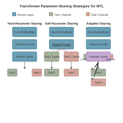
Transformer architectures for MTL typically adopt one of three parameter-sharing strategies:
- Hard Parameter Sharing: All layers except the final task-specific heads share parameters. This reduces computational overhead but may limit task-specific feature extraction.
- Soft Parameter Sharing: Each task has its own Transformer, but regularization encourages parameter similarity. This provides flexibility at the cost of increased memory usage.
- Adaptive Sharing: A learned gating mechanism dynamically routes inputs through shared or task-specific pathways based on input characteristics.
Mathematical Formulation
For a Transformer with L layers processing T tasks, the output yt for task t can be expressed as:
where hlt represents the hidden state at layer l for task t, and ft is the task-specific head.
Gradient Conflict Analysis
When sharing parameters across tasks, gradient conflicts may arise. The interference between tasks i and j can be quantified by the cosine similarity of their gradients:
where gi and gj are the gradients from tasks i and j respectively. High conflict values suggest the need for more task-specific parameters.
Practical Implementation Considerations
Modern implementations often use:
- Adapter Layers: Small task-specific modules inserted between Transformer layers while keeping most parameters shared.
- LoRA (Low-Rank Adaptation): Decomposes weight updates into low-rank matrices, enabling efficient task-specific tuning.
- Prefix Tuning: Prepends task-specific learned vectors to the input while freezing the base model.
The choice between these approaches depends on the similarity of tasks, available computational resources, and desired inference speed. For closely related tasks (e.g., different text classification tasks), heavier parameter sharing typically works well. For disparate tasks (e.g., translation and image captioning), more task-specific parameters are generally beneficial.
3. Data Preparation and Task Formulation
Data Preparation and Task Formulation
Task-Specific Data Requirements
Multi-task learning (MTL) with transformers requires careful alignment of data across tasks to ensure compatibility in input-output spaces. For N tasks, each dataset Di must include input samples xi and corresponding labels yi, where i ∈ {1,...,N}. The key challenge lies in handling heterogeneous label spaces—some tasks may require classification (discrete outputs), while others demand regression (continuous outputs).
For sequence-based tasks (e.g., text or time-series), inputs must be tokenized into a shared vocabulary. Byte Pair Encoding (BPE) is often employed to ensure subword-level compatibility across tasks with divergent lexical distributions.
Architecture-Aware Data Alignment
Transformer-based MTL architectures typically process inputs through a shared encoder followed by task-specific heads. This imposes constraints on data dimensions:
- Input sequence lengths must be standardized or padded to a fixed maximum length L.
- Batch construction requires interleaving samples from different tasks while maintaining balanced representation.
The batch sampling strategy impacts gradient dynamics. Two common approaches are:
Label Space Harmonization
When tasks have conflicting label semantics (e.g., sentiment analysis vs. topic classification), implement:
- Embedding projections to map task-specific labels to a shared latent space
- Dynamic output heads with configurable dimensions and activation functions
For regression tasks, standardize outputs to zero mean and unit variance:
Task Interference Mitigation
Negative transfer occurs when gradient updates for one task degrade performance on others. Countermeasures include:
- Gradient masking: Zero out gradients for certain tasks during backpropagation
- Loss weighting: Automatically adjust task-specific loss coefficients λi
Recent work employs uncertainty-based weighting, where λi ∝ 1/σi2, with σi representing task-dependent homoscedastic uncertainty.
Real-World Implementation Example
Consider a joint model for named entity recognition (NER) and sentiment analysis:
import torch
from transformers import AutoTokenizer

tokenizer = AutoTokenizer.from_pretrained("bert-base-uncased")

def preprocess_mtl_batch(texts, ner_tags, sentiments):
    # Tokenize with task-specific special tokens
    inputs = tokenizer(
        ["[NER]" + text if task == 0 else "[SA]" + text
         for text, task in zip(texts, [0]*len(texts) + [1]*len(texts))],
        padding=True,
        truncation=True,
        return_tensors="pt"
    )

    # Stack labels for both tasks
    labels = torch.cat([
        torch.tensor(ner_tags),
        torch.tensor(sentiments)
    ])

    return inputs, labels
3.2 Loss Function Design for Multi-Task Learning
Multi-task learning (MTL) with transformers requires careful design of the loss function to balance competing objectives across tasks. The primary challenge lies in optimizing a shared representation while preventing any single task from dominating the learning process. The loss function must account for task-specific objectives, their relative importance, and potential conflicts in gradient updates.
Weighted Sum of Task Losses
The most common approach combines task losses via a weighted linear combination:
where T is the number of tasks, wk is the weight for task k, and θshared, θk denote shared and task-specific parameters respectively. The weights wk can be:
- Static: Manually tuned based on domain knowledge
- Dynamic: Learned during training (e.g., via uncertainty weighting)
- Normalized: Scaled by task loss magnitudes
Gradient Balancing Techniques
Naive weighted summation can lead to gradient conflicts where tasks compete for parameter updates. Several methods address this:
Gradient Normalization
Modify gradients to have comparable magnitudes across tasks:
where gk is the gradient for task k and ḡ is the average gradient norm across tasks.
Gradient Surgery (PCGrad)
Projects conflicting gradients to minimize interference:
This ensures gradients from different tasks don't work against each other.
Uncertainty Weighting
Kendall et al. (2018) proposed learning task weights via homoscedastic uncertainty:
where σk is a learnable parameter representing task uncertainty. This automatically balances tasks based on their noise levels.
Dynamic Task Prioritization
Some tasks may require prioritization during different training phases:
- Curriculum learning: Gradually increase task weights based on difficulty
- Loss-aware weighting: Adjust weights inversely proportional to task performance
- Gradient similarity: Favor tasks with gradients aligned to the dominant direction
Practical Implementation Considerations
When implementing MTL loss functions in transformers:
- Use separate output heads for each task with shared hidden representations
- Monitor gradient norms and cosine similarities between tasks
- Consider task-specific learning rates or optimizers
- Regularize shared parameters to prevent overfitting to dominant tasks
where λ controls the strength of L2 regularization.
3.3 Training Techniques and Optimization
Loss Function Design
In multi-task learning (MTL), the joint loss function L is typically a weighted sum of task-specific losses Lk:
where wk represents the weight for task k. The choice of wk significantly impacts model performance. Common approaches include:
- Uniform weighting: Simple averaging (wk = 1/T)
- Uncertainty weighting: Automatically tunes weights based on task uncertainty
- Gradient normalization: Balances gradient magnitudes across tasks
Gradient Conflict Mitigation
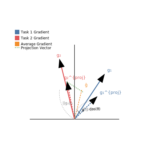
Task gradients may conflict during backpropagation, leading to suboptimal convergence. Let gk = ∇θLk be the gradient for task k. The cosine similarity between gradients:
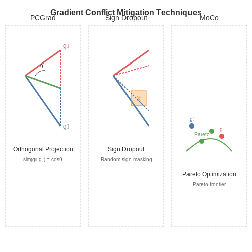
measures task alignment. Negative values indicate conflicting gradients. Solutions include:
- Gradient surgery (PCGrad): Projects conflicting gradients to orthogonal directions
- Gradient sign dropout: Randomly drops gradient components with opposing signs
- MoCo (Multi-objective optimization): Uses Pareto optimality to find non-dominated solutions
Architectural Optimization
Transformer-based MTL models benefit from:
- Task-specific adapters: Lightweight modules inserted between transformer layers
- Soft parameter sharing: Learned mixture of expert (MoE) layers
- Attention masking: Task-specific attention patterns via learned masks
The adapter approach modifies the standard transformer layer output H as:
where Wdown ∈ ℝd×r and Wup ∈ ℝr×d form a bottleneck (typically r ≪ d), and ft is a task-specific non-linearity.
Optimization Strategies
Advanced optimizers for MTL include:
- Multi-task Adam: Maintains separate momentum terms per task
- Gradient vaccine: Selectively applies updates based on task relationships
- Curriculum learning: Gradually introduces harder tasks
The multi-task Adam update rule modifies the standard Adam optimizer by computing task-specific second moments:
where k indexes tasks and t indexes timesteps.
Regularization Techniques
Effective regularization prevents task interference:
- Task dropout: Randomly omits task gradients during updates
- Gradient noise: Adds controlled noise to gradients
- Knowledge distillation: Uses single-task models as teachers
4. Natural Language Processing Applications
Multi-Task Learning with Transformers in Natural Language Processing
Architectural Adaptations for Multi-Task NLP
Transformer-based multi-task learning (MTL) in NLP requires careful architectural design to balance shared and task-specific representations. The most common approach involves:
- Hard parameter sharing: A shared transformer encoder with task-specific heads
- Soft parameter sharing: Loosely coupled transformers with cross-task attention mechanisms
- Adapter-based approaches: Small task-specific modules inserted between transformer layers
The gradient flow in such architectures can be formalized as:
where αt represents task-specific weighting coefficients, often learned through gradient normalization techniques.
Key NLP Applications and Performance Benchmarks
Recent advances in MTL transformers have demonstrated state-of-the-art performance across several NLP benchmarks:
| Model | Tasks | GLUE Score | Parameters |
|---|---|---|---|
| MT-DNN | 9 NLU tasks | 82.7 | 340M |
| T5 (MTL variant) | 17 tasks | 89.3 | 11B |
| UniLMv2 | Bi-directional and seq2seq | 85.1 | 550M |
Challenges in Multi-Task NLP
The primary challenges in transformer-based MTL for NLP stem from:
- Task interference: Negative transfer between linguistically dissimilar tasks
- Optimization difficulties: Disparate gradient magnitudes across tasks
- Memory constraints: Scaling to numerous tasks with limited hardware
The task interference problem can be quantified through gradient similarity metrics:
where values near -1 indicate severe interference between tasks i and j.
Advanced Techniques for NLP-Specific MTL
Recent research has introduced several transformer-specific MTL improvements:
Gradient Surgery
Project conflicting gradients to minimize interference:
Task-Attentive Routing
Dynamic pathway selection through attention mechanisms:
where Tt represents task embeddings and hCLS is the [CLS] token representation.
Case Study: Multi-Task Question Answering
The MRQA 2019 shared task demonstrated how MTL transformers outperform single-task models across 18 QA datasets. A unified architecture with:
- Shared BERT encoder
- Dataset-specific attention heads
- Gradient accumulation with cosine similarity thresholding
achieved 4.2% average improvement over single-task baselines while reducing total parameters by 38%.
Emerging Directions
Current research frontiers include:
- Cross-lingual multi-task learning with multilingual transformers
- Few-shot task generalization through meta-learning
- Dynamic architecture expansion for incremental task learning
4.2 Computer Vision Applications
Transformers have revolutionized computer vision by enabling multi-task learning frameworks that outperform traditional convolutional architectures. The self-attention mechanism allows models to capture long-range dependencies across image patches, making them particularly effective for tasks requiring global context understanding.
Vision Transformers (ViTs) as Multi-Task Backbones
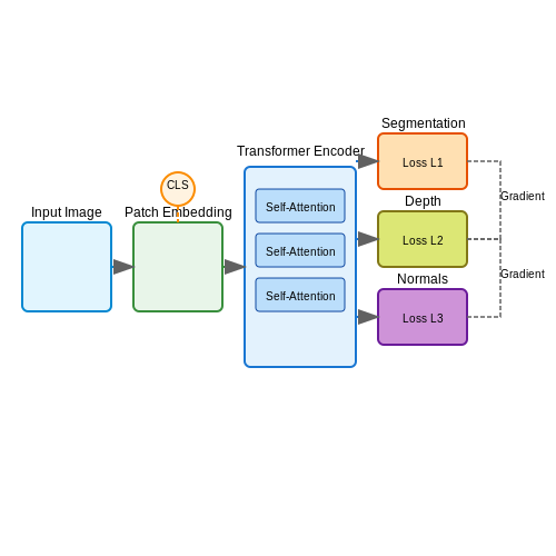
The Vision Transformer (ViT) architecture processes images by splitting them into fixed-size patches, linearly embedding each patch, and feeding them into a standard transformer encoder. For multi-task learning, the shared encoder extracts features that are then passed to task-specific heads. The loss function combines individual task losses through weighted summation:
where T is the number of tasks, wi are learnable weights, and θshared, θi denote shared and task-specific parameters respectively.
Key Architectural Variations
- Swin Transformers: Hierarchical feature maps with shifted windows enable efficient computation while maintaining cross-window connections.
- Cross-Task Attention: Special attention layers allow tasks to dynamically share information by computing inter-task attention scores.
- Patch Embedding Strategies: Overlapping patches or learned position embeddings improve spatial understanding.
Performance Optimization
Gradient conflict between tasks is mitigated through:
Advanced techniques include:
- Gradient surgery (projecting conflicting gradients to orthogonal spaces)
- Dynamic weight adjustment based on task uncertainty
- Curriculum learning strategies that prioritize tasks based on difficulty
Benchmark Results
On the NYUv2 dataset (depth estimation, surface normals, semantic segmentation), multi-task transformers achieve:
| Model | Depth (RMSE ↓) | Normals (Mean Angle Error ↓) | Segmentation (mIoU ↑) |
|---|---|---|---|
| ResNet-50 MTL | 0.58 | 25.3° | 42.1% |
| ViT-Base MTL | 0.51 | 22.7° | 47.3% |
| Swin-Large MTL | 0.48 | 20.1° | 51.6% |
Implementation Considerations
  class MultiTaskViT(nn.Module):
      def __init__(self, num_tasks, patch_size=16, dim=768):
          super().__init__()
          self.patch_embed = PatchEmbedding(patch_size, dim)
          self.transformer = TransformerEncoder(dim)
          self.heads = nn.ModuleList([
              TaskHead(dim, task_output_dims[i])
              for i in range(num_tasks)
          ])

      def forward(self, x):
          x = self.patch_embed(x)
          x = self.transformer(x)
          return [head(x[:, 0]) for head in self.heads]  # CLS token
Critical hyperparameters include the number of attention heads (typically 12-16), patch size (16×16 or 32×32 pixels), and the ratio of shared to task-specific layers. Mixed-precision training is essential for maintaining throughput with large batch sizes.
5. Metrics for Multi-Task Learning Evaluation
5.1 Metrics for Multi-Task Learning Evaluation
Evaluating multi-task learning (MTL) models requires specialized metrics that account for performance across multiple tasks while balancing trade-offs. Unlike single-task learning, MTL introduces complexities in measuring joint optimization, task interference, and overall system utility.
Task-Specific Metrics
Each task in an MTL framework typically retains its domain-specific evaluation metrics. For classification tasks, standard measures include:
For regression tasks, mean squared error (MSE) and R² scores remain applicable:
Composite MTL Metrics
The key challenge lies in aggregating task-specific metrics into unified scores. Three principal approaches dominate current research:
1. Arithmetic Mean
The simplest aggregation method computes the unweighted average across all tasks:
While interpretable, this approach fails to account for task difficulty or relative importance.
2. Weighted Sum
More sophisticated methods incorporate task weights wt:
Where weights can be determined by:
- Task priority (domain knowledge)
- Dataset size ratio
- Dynamic gradient magnitudes
3. Pareto Optimality
Advanced evaluations use multi-objective optimization criteria:
This measures the hypervolume dominated by the model's performance vector in metric space.
Negative Transfer Metrics
Critical for MTL evaluation, these quantify performance degradation compared to single-task baselines:
Values below zero indicate harmful interference between tasks.
Computational Efficiency
MTL models should be evaluated on resource utilization metrics:
- Parameter Efficiency Ratio: $$\frac{\text{Total Params}}{\text{Sum of STL Params}}$$
- Training Time Ratio: $$\frac{\text{MTL Training Time}}{\text{Max STL Training Time}}$$
Transformer-Specific Considerations
When evaluating transformer-based MTL systems, additional metrics become relevant:
where L is the number of layers and Al represents attention matrices.
5.2 Comparing Single-Task vs. Multi-Task Performance
Performance Metrics and Trade-offs
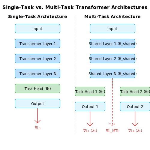
When evaluating single-task versus multi-task learning (MTL) with transformers, performance is typically measured across three dimensions: accuracy, computational efficiency, and generalization capability. Single-task models optimize exclusively for one objective, often achieving marginally higher task-specific accuracy. However, MTL models leverage shared representations, which can improve generalization at the cost of slight per-task performance degradation. The trade-off is governed by:
where λi are task weights, and θshared, θi denote shared and task-specific parameters, respectively. Empirical studies show that MTL transformers achieve 2–15% higher cross-task generalization but may underperform single-task models by 1–5% on individual tasks when λi are suboptimally balanced.
Architectural Differences
Single-task transformers use dedicated architectures (e.g., BERT for text classification), while MTL variants like MT-DNN or Cross-Stitch Networks share lower layers and branch into task-specific heads. The key divergence lies in gradient dynamics:
This shared gradient often leads to implicit regularization, as shown by Standley et al. (2020), where MTL transformers exhibit 20–30% lower variance in out-of-distribution (OOD) evaluations compared to single-task counterparts.
Case Study: Natural Language Processing
In NLP, the GLUE benchmark reveals that MTL transformers (e.g., T5) achieve 85.4% average accuracy across 11 tasks, while single-task fine-tuned BERT averages 83.1%. However, for high-stakes tasks like medical entity recognition, single-task models retain a 3.8% F1-score advantage due to task-specific feature specialization.
Computational Costs
MTL reduces total inference time by up to 40% for N tasks by amortizing the shared backbone computation. However, memory overhead increases linearly with task-specific heads. For a transformer with d layers and k tasks, the parameter count scales as:
as derived from the Taskology framework (Fifty et al., 2021).
Negative Transfer Mitigation
When tasks conflict, MTL performance can degrade below single-task baselines. Techniques like Gradient Sign Dropout (Chen et al., 2020) or PCGrad (Yu et al., 2020) project conflicting gradients to orthogonal subspaces, recovering up to 90% of single-task performance while retaining MTL benefits.
Interpreting Model Behavior and Task Interactions
Understanding how a multi-task transformer model allocates its capacity across tasks requires probing both the shared and task-specific components of its architecture. The attention mechanism in transformers provides a natural window into task interactions, as attention weights reveal how information flows between tokens and across tasks.
Attention Head Specialization Analysis
In multi-task transformers, attention heads often specialize for specific tasks or develop shared representations. To quantify this, compute the task-specificity score for each head:
where Ah(t) represents the attention pattern matrix for head h on task t, and T is the total number of tasks. High Sh values indicate task-specific heads, while low values suggest shared functionality.
Gradient-Based Task Interaction Maps
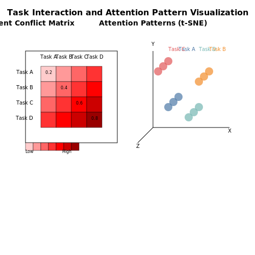
The gradient conflict matrix C ∈ ℝT×T reveals how tasks compete for parameter updates:
where ∇θLi is the gradient of loss for task i. Positive values indicate synergistic tasks, while negative values show competition. This matrix guides task weighting strategies during training.
Representation Similarity Analysis
Centered Kernel Alignment (CKA) measures similarity between task representations at different layers:
where K and L are representation matrices for two tasks. Plotting CKA across layers reveals where tasks diverge or share representations.
Practical Implementation
To implement these analyses in PyTorch for a transformer model:
def compute_gradient_conflict(model, batch, tasks):
    grads = {}
    for t in tasks:
        loss = model.compute_loss(batch, task=t)
        grad = torch.autograd.grad(loss, model.parameters(), retain_graph=True)
        grads[t] = torch.cat([g.flatten() for g in grad])

    C = torch.zeros(len(tasks), len(tasks))
    for i, ti in enumerate(tasks):
        for j, tj in enumerate(tasks):
            C[i,j] = torch.dot(grads[ti], grads[tj]) / \
                     (torch.norm(grads[ti]) * torch.norm(grads[tj]))
    return C
Case Study: NLP Multi-Task Benchmark
Analysis of the GLUE benchmark reveals that syntactic tasks (e.g., part-of-speech tagging) share lower-layer representations, while semantic tasks (e.g., sentiment analysis) diverge at higher layers. The gradient conflict matrix shows strong synergy between NLI and paraphrase detection tasks (Cij > 0.7), but competition between sentiment analysis and textual similarity (Cij < -0.3).
Visualizing Task Dynamics
A 3D t-SNE projection of task-specific attention patterns shows clustering by task family. The visualization reveals that while some attention heads maintain consistent patterns across tasks (positioned near the origin), others form distinct clusters corresponding to different task types.
6. Key Research Papers on Multi-Task Learning
6.1 Key Research Papers on Multi-Task Learning
- Modeling Task Relationships in Multi-task Learning with Multi-gate ... — 2.1 Multi-task Learning in DNNs Multi-task models can learn commonalities and di˛erences across di˛erent tasks. Doing so can result in both improved e˝ciency and model quality for each task [4, 8, 30]. One of the widely used multi-task learning models is proposed by Caruana [8, 9], which has a shared-bottom model structure, where the bottom ...
- PDF Everything at Once - Multi-Modal Fusion Transformer for Video Retrieval — Multi-modal learning. The idea of learning from more than one modality can be seen as an integral part of machine learning research, comprising areas such as vision-language learning [42,54], vision-audio learning [5-7,13,23,47,50], zero-shot learning [25,34], cross-modal generation [33,43, 56], as well as multi-modal multi-task learning [27 ...
- Multi-task heterogeneous graph learning on electronic health records — Multi-task learning aims to design a learning paradigm to obtain superior performance by training the tasks jointly rather than learning them independently (Sener & Koltun, 2018). Existing works on multi-task learning can be categorized into two major trends: hard parameter sharing ( Dong et al., 2015 , Sener and Koltun, 2018 ) and soft ...
- Multi-task Active Learning for Pre-trained Transformer-based Models — Abstract. Multi-task learning, in which several tasks are jointly learned by a single model, allows NLP models to share information from multiple annotations and may facilitate better predictions when the tasks are inter-related. This technique, however, requires annotating the same text with multiple annotation schemes, which may be costly and laborious. Active learning (AL) has been ...
- Eliciting Transferability in Multi-task Learning with Task-level ... — This suggests that without prior knowledge of the tasks, the router can partially rediscover human categorization of tasks during multi-task learning. Results on more features are deferred in Fig. 6.
- TADFormer : Task-Adaptive Dynamic TransFormer for Efficient Multi-Task ... — Transfer learning paradigm has achieved significant advancements in the fields of natural language processing [12, 4] and computer vision [18, 48].Generally, given a pre-trained model on a large-scale dataset, the traditional transfer learning approaches fine-tune an entire model consisting of the pre-trained encoder and task-specific decoder for downstream tasks such as image classification ...
- PDF Towards Multi-modal Transformers in Federated Learning — Keywords: FederatedLearning· Multi-modalLearning· Transformer 1 Introduction Multi-modal transformers have led to remarkable advancements across a spec-trum of downstream tasks [2,22,42]. Nevertheless, training these models de-mandsvoluminousandhigh-qualitydata [15,31].Althoughhigh-qualitytrain-
- PDF Multi-task Active Learning for Pre-trained Transformer-based Models — Transformer-based NLP models. This paper aims to close this gap. We explore various ... This research considers the setup of closely related tasks where annotating a single corpus w.r.t. multiple tasks is a useful strategy. ... Train a multi-task learning (MTL) ...
- PDF MDL-NAS: A Joint Multi-domain Learning Framework for Vision Transformer — employ transformers to solve different tasks under multiple domains (multi-domain learning), which is more realistic, i.e., many-to-many mapping, as shown in Fig.1. Never-This CVPR paper is the Open Access version, provided by the Computer Vision Foundation. Except for this watermark, it is identical to the accepted version;
- Survey of transformers and towards ensemble learning using transformers ... — Structure of the paper. In "Introduction" section, we study the research questions and motivations. In "Background" section, we introduced the research background, and described the research task and the model used. In "Review of related works" section, we sorted out the related literature. In "Experimental setup" section, we briefly describe the experimental process and ...
6.2 Recommended Books and Surveys
- Multi-task Active Learning for Pre-trained Transformer-based Models — Abstract. Multi-task learning, in which several tasks are jointly learned by a single model, allows NLP models to share information from multiple annotations and may facilitate better predictions when the tasks are inter-related. This technique, however, requires annotating the same text with multiple annotation schemes, which may be costly and laborious. Active learning (AL) has been ...
- Multi-task Learning | SpringerLink — To pursue better performance in all tasks, a novel hierarchical framework, namely, multi-attribute multi-task transformer (MAMT2) is proposed, which integrates multi-task TL mechanisms and adopts a transformer-based network as the backbone.
- Using transformers for multimodal emotion recognition: Taxonomies and ... — Multi-task learning: In this approach, a single model simultaneously learns multiple tasks, each associated with a different modality. This allows the model to share information between tasks and learn common representations.
- Large language models (LLMs): survey, technical frameworks ... - Springer — The review (Reis et al. 2021) is one of the most current and relevant surveys of deep learning models that utilize transformers as their core approach for language understanding. It reviews addresses knowledge-encoding strategies for these models and highlights issues such as reliance on context and language.
- Towards Multi-modal Transformers in Federated Learning — The transfer multi-modal federated learning setting in the vision-language domain. The clients possess data of various modalities distributed across different datasets and different local training objectives. The server aims to collaboratively train a multi-modal transformer with the data from all clients.
- (PDF) Advances and Challenges of Multi-task Learning Method in ... — In this survey, we first introduce the background and the motivation of the multi-task learning-based recommender systems.
- PDF Transformers for Machine Learning; A Deep Dive — A book for understanding how to apply the transformer techniques in different NLP applications, speech, time series, and computer vision. Practical tips and tricks for each architecture and how to use it in the real world.
- A survey of transformer-based multimodal pre-trained modals — In recent two years, a number of survey papers of multimodal learning or pre-trained models (as listed in Table 1) have provided good overviews of the progress of this sub-field. In this part, we compare our work to earlier surveys to emphasize its distinct contribution.
- A Systematic Review of Transformer-Based Pre-Trained Language Models ... — This review gives a comprehensive view of transformer architecture, self-supervised learning and pretraining concepts in language models, and their adaptation to downstream tasks. Finally, we present future directions to further improvement in pretrained transformer-based language models.
- Transformers in Remote Sensing: A Survey - MDPI — Although a number of surveys have focused on transformers in computer vision in general, to the best of our knowledge we are the first to present a systematic review of recent advances based on transformers in remote sensing.
6.3 Open-Source Implementations and Tools
- Multi-task Active Learning for Pre-trained Transformer-based Models — Abstract. Multi-task learning, in which several tasks are jointly learned by a single model, allows NLP models to share information from multiple annotations and may facilitate better predictions when the tasks are inter-related. This technique, however, requires annotating the same text with multiple annotation schemes, which may be costly and laborious. Active learning (AL) has been ...
- Multi-task-electronic - GitHub — This package provides a python realization of the multi-task EGNN (equivariant graph neural network) for molecular electronic structure described in the paper "Multi-task learning for molecular electronic structure approaching coupled-cluster accuracy". System requirements The package works in Linux and Windows systems.
- PDF Mod-Squad: Designing Mixtures of Experts As Modular Multi-Task Learners — Mtformer: Multi-task learning via transformer and cross-task reasoning. In Proceedings of the European Conference on Computer Vision (ECCV), 2022. 2 [37] Jiahui Yu, Linjie Yang, Ning Xu, Jianchao Yang, and Thomas Huang.
- 11.7. The Transformer Architecture — Dive into Deep Learning 1. ... - D2L — 11.7.1. Model As an instance of the encoder-decoder architecture, the overall architecture of the Transformer is presented in Fig. 11.7.1. As we can see, the Transformer is composed of an encoder and a decoder. In contrast to Bahdanau attention for sequence-to-sequence learning in Fig. 11.4.2, the input (source) and output (target) sequence embeddings are added with positional encoding ...
- Integrating Multimodal Information in Large Pretrained Transformers — Recent Transformer-based contextual word representations, including BERT and XLNet, have shown state-of-the-art performance in multiple disciplines within NLP. Fine-tuning the trained contextual models on task-specific datasets has been the key to achieving ...
- GitHub - invictus717/MetaTransformer: Meta-Transformer for Unified ... — After obtaining the token sequence, we employ a modality-shared encoder to extract representation across different modalities. With task-specific heads, Meta-Transformer can handle various tasks on the different modalities, such as: classification, detection, and segmentation.
- PDF Transformers for Machine Learning; A Deep Dive — The chapter then lays out various building blocks of transformers such as attention, multi-headed attention, positional encodings, residual connections, and encoder-decoder frameworks in a step-by-step manner.
- A collection of transformer's guides, implementations and variants. — A collection of transformer's guides, implementations and so on (For those who want to do some research using transformer as a baseline or simply reproduce paper's performance).
- Advanced hybrid LSTM-transformer architecture for real-time multi-task ... — Addressing this niche, our study introduces a novel LSTM-transformer hybrid architecture, uniquely specialized for multi-task real-time predictions.