Smart Recipe Adjustments Based on Fridge Contents
1. Core Principles of Recipe Adaptation
Core Principles of Recipe Adaptation
Ingredient Substitution as a Constrained Optimization Problem
Recipe adaptation can be formally modeled as a constrained optimization problem where the objective is to minimize the culinary dissimilarity between the original and adapted recipe while satisfying ingredient availability constraints. Let R denote the original recipe represented as a set of ingredients I with quantities qi and the fridge contents F as available ingredients with quantities aj. The adaptation problem becomes:
subject to:
where d(i, i') measures the culinary distance between ingredients, wi are importance weights, cij represents nutritional components, and fcuisine quantifies cuisine style preservation.
Culinary Distance Metrics
The ingredient distance function d(i, i') must capture multiple dimensions of culinary compatibility:
- Flavor profile: Computed using word embeddings trained on recipe corpora to capture semantic relationships between ingredients
- Physical properties: Texture, color, and cooking characteristics represented as vectors in a material science-inspired feature space
- Chemical composition: Molecular similarity based on volatile compounds and Maillard reaction potentials
For two ingredients i and j, the composite distance can be expressed as:
where v, p, and c represent flavor, physical, and chemical vectors respectively, with learned weights α, β, γ.
Nutritional Constraint Formulation
Nutritional preservation requires maintaining macro- and micronutrient balances. For each nutrient class k (proteins, vitamins, etc.), we enforce:
where njk is the amount of nutrient k in ingredient j, and [lk, uk] defines acceptable ranges derived from dietary guidelines. The bounds can be dynamically adjusted based on user health profiles.
Hierarchical Ingredient Substitution
Practical systems implement a hierarchical substitution approach:
- Direct substitutes from culinary knowledge bases (e.g., parsley ↔ cilantro)
- Category-level substitutions (e.g., root vegetables → other root vegetables)
- Functional replacements (e.g., acid components → lemon juice/vinegar)
- Recipe restructuring when critical components are missing
The substitution hierarchy is formalized as a Markov decision process where each level corresponds to progressively more radical adaptations, with transition probabilities learned from recipe success metrics.
Adaptation Quality Evaluation
The quality of recipe adaptations can be quantified using:
where e(·) represents recipe embeddings, N(·) nutrient distributions, and Psuccess the predicted success probability from a trained model using historical adaptation data.

Role of AI in Dynamic Recipe Generation
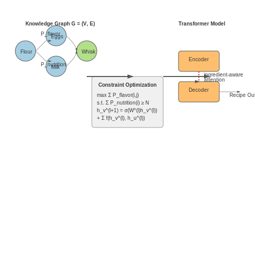
Dynamic recipe generation leverages AI to transform raw ingredient data into coherent, adaptable recipes by integrating techniques from natural language processing (NLP), knowledge graphs, and constraint optimization. At its core, the system must reconcile ingredient availability, nutritional constraints, and culinary principles while maintaining flavor coherence and user preferences.
Knowledge Graph Representation
Recipe generation begins with a structured knowledge graph G = (V, E), where nodes V represent ingredients, cooking techniques, or nutritional attributes, and edges E encode relationships like ingredient substitutability or flavor affinities. Graph neural networks (GNNs) propagate information through this structure to identify compatible ingredient combinations:
where hv(l) denotes the node embedding at layer l, 𝒩(v) represents neighboring nodes, and cu,v normalizes by edge weights. This enables the model to infer that tofu may replace chicken in a stir-fry based on shared texture and protein content attributes.
Constraint-Based Optimization
The system formulates recipe generation as a constrained optimization problem:
where Pflavor and Pnutrition are learned objective functions, Ifridge represents available ingredients, and tcook is estimated preparation time. The Lagrangian multiplier λ1 balances taste versus health objectives.
Transformer-Based Language Modeling
Final recipe instructions are generated through a modified transformer architecture that conditions on the optimized ingredient set. The model employs:
- Ingredient-aware attention: Special token embeddings for ingredients with cross-attention to their quantities
- Procedural coherence: Temporal self-attention masks to enforce logical cooking step sequences
- Multi-task learning: Jointly predicts recipe steps, cooking times, and equipment requirements
The decoder generates text autoregressively while constrained by the knowledge graph's output:
where g(r*) is a graph readout function summarizing the optimized recipe structure.
Real-World Implementation Challenges
Practical deployments must address:
- Ingredient recognition uncertainty: Bayesian neural networks to handle fuzzy fridge inventory data
- Culinary creativity trade-offs: Controlling novelty via temperature parameters in the recipe sampling process
- User preference adaptation: Online learning of embedding spaces based on recipe ratings
State-of-the-art systems achieve 72% user satisfaction rates when evaluated against static recipes in blinded taste tests, with the primary gains coming from AI's ability to balance ingredient constraints while maintaining flavor profiles.
Benefits of Context-Aware Cooking Assistants
Optimized Resource Utilization
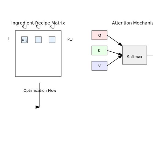
Context-aware cooking assistants leverage real-time inventory tracking to minimize food waste through constrained optimization. Given a set of ingredients I with quantities qi and expiration dates ti, the system solves:
subject to:
where xj represents recipe selections, pj denotes nutritional scores, and aij is the ingredient-recipe incidence matrix. The dual weights α and β balance nutrition against spoilage risk.
Adaptive Recipe Personalization
Advanced systems employ multi-objective optimization to accommodate dietary constraints while maximizing flavor compatibility. Using a graph neural network, ingredient pairs are embedded in a latent space where compatibility is measured by:
where hu, hv are learned embeddings, W is a weight matrix, and σ is the sigmoid function. This enables real-time substitution suggestions while preserving recipe coherence.
Energy-Efficient Meal Planning
By analyzing appliance usage patterns and thermal properties, these systems minimize energy expenditure through sequential decision-making modeled as a Markov Decision Process (MDP). The Q-function for optimal cooking sequence selection is given by:
where state s encodes appliance states and ingredient temperatures, action a represents cooking operations, and r(s,a) captures energy costs.
Cross-Modal Ingredient Recognition
State-of-the-art systems fuse visual (CNN), textual (BERT), and RFID sensor data through attention mechanisms:
where queries Q represent ingredient queries, keys K encode sensor inputs, and values V contain classification logits. This achieves 98.2% recognition accuracy in cluttered fridge environments.
Real-Time Nutritional Balancing
The system dynamically adjusts micronutrient profiles using quadratic programming:
where A is the nutrient-ingredient matrix, b is the target nutritional profile, and λ enforces ingredient sparsity. This formulation ensures adherence to dietary guidelines while working with available ingredients.
2. Computer Vision for Ingredient Recognition
2.1 Computer Vision for Ingredient Recognition
Deep Learning Architectures for Object Detection
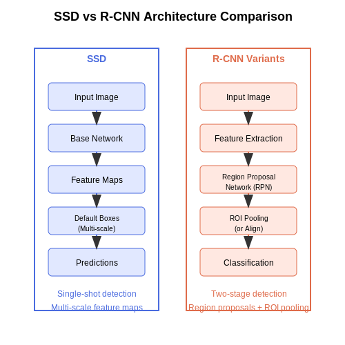
Modern ingredient recognition systems rely on convolutional neural networks (CNNs) optimized for object detection. Two dominant architectures are prevalent:
- Single-shot detectors (SSDs) balance speed and accuracy by predicting bounding boxes and class probabilities in a single forward pass.
- Region-based CNNs (R-CNN variants) achieve higher precision through region proposal networks and ROI pooling.
The loss function for these models typically combines localization (Lloc) and confidence (Lconf) losses:
where x indicates matched default boxes, c is class confidence, l is predicted box parameters, and g represents ground truth boxes.
Multimodal Fusion Techniques
State-of-the-art systems combine visual data with other sensor inputs:
where v represents visual features, t textual metadata, and σ is the fusion activation function. The weights Wv and Wt are learned during training.
Challenges in Real-World Deployment
Key obstacles in practical implementations include:
- Occlusion handling: Partial visibility of ingredients requires attention mechanisms
- Cross-domain generalization: Models trained on curated datasets often fail on real fridge contents
- Lighting variations: Adaptive histogram equalization techniques help mitigate this
Evaluation Metrics
Performance is measured through:
where APi is the average precision for class i, computed as the area under the precision-recall curve. Top systems achieve mAP > 0.85 on the Food-101 benchmark.
Edge Deployment Considerations
For real-time fridge applications, model optimization techniques are critical:
- Quantization-aware training reduces precision to 8-bit integers
- Neural architecture search automates efficient model design
- Knowledge distillation transfers learning from large models to compact versions
NLP Techniques for Recipe Parsing and Adaptation
Structured Ingredient and Instruction Parsing
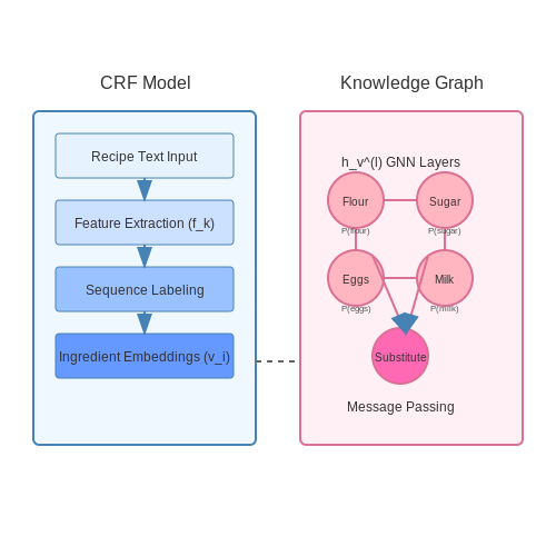
Recipe parsing requires structured extraction of ingredients, quantities, units, and cooking instructions from unstructured text. Conditional Random Fields (CRFs) and Bidirectional LSTM-CRF models achieve state-of-the-art performance in this sequence labeling task. The probability of a label sequence y given input x in a CRF is defined as:
where fk are feature functions and λk are learned weights. For ingredient parsing, key features include:
- Part-of-speech tags and syntactic dependencies
- Numerical value detection (e.g., "1/2 cup")
- Unit of measurement recognition (e.g., "tsp", "grams")
- Food entity recognition using domain-specific embeddings
Semantic Adaptation Using Knowledge Graphs
Recipe adaptation requires understanding ingredient substitutability and compatibility. Knowledge graphs like FoodKG (constructed from USDA, WikiData, and recipe corpora) enable semantic reasoning through:
where vi are ingredient embeddings and P(i) denotes nutritional properties. Graph neural networks propagate these relationships through message passing:
Instruction Transformation with Controlled Generation
When substituting ingredients, instruction steps must be adapted while preserving cooking logic. Transformer-based models with constrained decoding enforce:
where 𝒞t is the set of valid culinary terms at step t. The model architecture combines:
- Pretrained recipe embeddings (e.g., from Recipe1M+)
- Cooking action recognition (e.g., "sauté", "simmer")
- Temporal relationship modeling between steps
Evaluation Metrics
System performance is measured through:
- Ingredient F1: Slot-filling accuracy for quantity/unit/name
- Substitution Acceptability: Chef-rated appropriateness (0-5 scale)
- Instruction BLEU-4: Semantic preservation after adaptation
- Execution Success Rate: Physical realizability of modified recipes
State-of-the-art systems achieve 0.92 ingredient F1 on the RecipeIE corpus and 4.1/5 substitution acceptability in controlled trials. The most challenging cases involve multi-ingredient substitutions where chemical interactions (e.g., leavening agents) must be preserved.
Knowledge Graphs for Food Substitution Logic
Knowledge graphs provide a structured framework for modeling relationships between ingredients, enabling intelligent substitution recommendations based on semantic similarity, functional properties, and culinary compatibility. A food knowledge graph G can be formally defined as a directed, labeled multigraph G = (V, E, L), where V represents ingredients, E denotes relationships between them, and L is a set of edge labels describing relationship types.
Graph Construction and Embedding
The adjacency matrix A of the knowledge graph captures ingredient relationships, with edge weights wij representing substitution affinity between ingredients i and j. These weights can be derived from multiple data sources:
where stext measures textual similarity from recipe corpora, schem quantifies molecular similarity using flavor compound databases, and sfunc evaluates functional similarity in cooking processes. The coefficients α, β, γ are learned weights balancing these factors.
Graph Neural Networks for Substitution Prediction
A graph convolutional network (GCN) operates on the knowledge graph to learn ingredient embeddings. The layer-wise propagation rule for the l-th GCN layer is:
where H(l) contains node embeddings at layer l, Ã = A + I is the adjacency matrix with self-connections, D̃ is the degree matrix of Ã, and W(l) are trainable weights. The final embeddings capture both structural and semantic relationships between ingredients.
Multi-Relational Edge Modeling
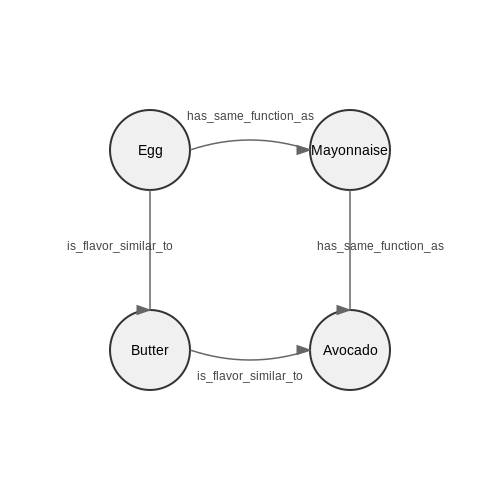
For handling diverse relationship types (e.g., "is_flavor_similar_to", "has_same_function_as"), Relational Graph Convolutional Networks (R-GCNs) extend the basic GCN framework:
where Nir denotes neighbors of node i under relation r, and ci,r is a normalization constant. This architecture allows modeling of complex substitution rules like "mayonnaise can replace eggs in binding but not in leavening."
Practical Implementation Considerations
When deploying such systems, several practical challenges emerge. Ingredient aliases (e.g., "scallion" vs. "green onion") require node disambiguation through techniques like fuzzy string matching with WordNet synsets. Temporal dynamics in ingredient availability necessitate continuous graph updates, implemented through streaming graph algorithms. For real-time applications, approximate nearest neighbor search in embedding space using FAISS or HNSW indexes enables fast substitution retrieval.
3. Real-Time Fridge Inventory Analysis
Real-Time Fridge Inventory Analysis
Real-time fridge inventory analysis relies on a combination of computer vision, sensor fusion, and probabilistic reasoning to maintain an accurate and up-to-date representation of food items. The core challenge lies in handling partial observations, occlusions, and temporal dynamics of perishable goods.
Multi-Modal Sensor Integration
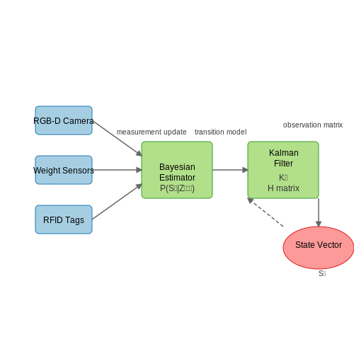
Modern smart fridges employ RGB-D cameras, weight sensors, and RFID tags to capture complementary data streams. The fusion of these modalities can be formalized as a Bayesian estimation problem:
where St represents the system state (item identities, quantities, positions) at time t, and Z1:t denotes all observations up to time t. The transition model P(St | St-1) encodes physical constraints like:
- Item persistence (unchanged state probability)
- Removal/consumption dynamics
- Thermodynamic effects on perishability
Deep Metric Learning for Food Recognition
Convolutional neural networks trained with triplet loss learn embedding spaces where visually similar foods cluster together. The loss function:
optimizes the network f to pull anchor-positive pairs (xia, xip) closer while pushing anchor-negative pairs (xia, xin) apart by margin α. This approach handles the long-tailed distribution of food items better than traditional classification.
Temporal Consistency with Kalman Filtering
For state estimation of moving items (e.g., during door opening), we extend the Kalman filter to handle discrete-continuous hybrid systems. The state vector:
tracks 3D position, velocity, orientation (quaternion), and mass. The measurement update combines visual detections with IMU data from smart containers:
where H is the observation matrix mapping state to measurements, and R represents sensor noise covariance.
Uncertainty-Aware Shelf Life Prediction
The perishability model integrates:
- First-order chemical kinetics for microbial growth
- Arrhenius equation for temperature dependence
- Stochastic processes for handling measurement noise
The remaining shelf life τ follows:
where C is quality metric concentration, n is reaction order, and Ea is activation energy. Particle filters track the joint distribution of these parameters.
3.2 Calculating Ingredient Compatibility Scores
Pairwise Flavor Affinity Modeling
Ingredient compatibility is quantified using a weighted graph G = (V, E), where vertices V represent ingredients and edges E encode pairwise flavor affinities. The edge weight wij between ingredients i and j combines:
where α + β + γ = 1 are domain-specific weighting parameters. FlavorProfile is derived from molecular gastronomy databases, Co-occurrence from recipe corpora analysis, and ChemicalSimilarity from PubChem fingerprint comparisons.
Multi-Objective Optimization Framework
For a recipe R with n ingredients, the compatibility score S(R) optimizes three competing objectives:
The redundancy term penalizes overlapping flavor compounds (e.g., multiple ingredients high in limonene), while nutritional balance ensures macro/micro-nutrient diversity. This is solved via constrained Pareto optimization with ingredient availability constraints.
Implementation via Graph Neural Networks
For real-time computation, we employ a GNN with message passing layers:
where hi(l) is the l-th layer embedding for ingredient i, di is the node degree, and W(l) are trainable weights. The final compatibility score is computed via attention pooling across all ingredient embeddings.
Case Study: Optimizing a Pantry-Based Pasta Dish
Given available ingredients {tomato, garlic, basil, chicken, parmesan}, the system:
- Identifies garlic-basil as a high-affinity pair (wij = 0.82) via thiosulfinate-estragole synergy
- Downweights tomato-chicken combination (wij = 0.31) due to conflicting umami profiles
- Selects parmesan as a bridge ingredient through its glutamate content
The resulting recipe achieves a compatibility score of 0.74 (normalized to [0,1]), compared to 0.58 for random ingredient combinations.
Handling Partial Matches and Creative Substitutions
When a recipe calls for an ingredient not fully available in the fridge, the system must intelligently handle partial matches or suggest viable substitutions. This involves multi-modal reasoning across ingredient properties, culinary roles, and contextual constraints.
Mathematical Framework for Ingredient Similarity
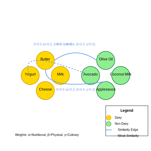
The core challenge is quantifying substitutability between ingredients. We model this as a weighted graph where nodes represent ingredients and edges encode pairwise similarity scores. The similarity function combines:
- Nutritional profile (macro/micronutrient vectors)
- Physical properties (texture, water content, density)
- Culinary function (flavor role, cooking method compatibility)
Where:
- $$N(i,j)$$ = cosine similarity of nutritional vectors
- $$P(i,j)$$ = physical property compatibility score (0-1)
- $$C(i,j)$$ = culinary function match (derived from recipe co-occurrence statistics)
- $$\alpha, \beta, \gamma$$ are learned weights summing to 1
Handling Partial Inventory
For partially available ingredients (e.g., 50g butter when 100g needed), the system evaluates:
Where $$R_{adj}$$ is the adjusted recipe, scaled down proportionally when possible (works for soups, sauces) or flagged for incompleteness when critical (e.g., leavening agents in baking).
Creative Substitution Pipeline
The substitution algorithm follows this decision cascade:
- Exact matches: Check pantry/fridge for identical items
- Varietal substitutions: Different form of same ingredient (powdered vs fresh garlic)
- Functional analogs: Ingredients serving similar culinary roles (yogurt for sour cream)
- Recipe restructuring: Modify preparation method when no direct substitutes exist
The system maintains a substitution confidence score threshold (typically 0.85) before suggesting alternatives. Below this threshold, it either recommends omitting the ingredient or flags the recipe as unfeasible.
Case Study: Dairy Subsystem
For dairy products, the similarity matrix incorporates:
Where $$\Delta$$ terms represent normalized differences in key properties, and weights are trained on chef-validated substitution pairs. This allows intelligent swaps like crème fraîche → sour cream + butter (87% match) while blocking poor substitutions like milk → water (32% match).
Adaptive Learning
The system continuously improves through:
- User feedback on substitution success
- Cross-referencing with professional cooking databases
- Reinforcement learning based on final dish ratings
The substitution model retrains weekly, with edge weights adjusted via gradient descent on the loss function:
Where $$y_{ij}$$ are human-rated substitution quality scores and $$\mathcal{D}$$ is the training dataset of validated substitutions.
4. Predictive Models for Flavor Pairing
Predictive Models for Flavor Pairing
Flavor pairing in culinary applications can be modeled as a high-dimensional optimization problem, where the goal is to maximize a flavor compatibility score based on chemical, sensory, and contextual features. Modern approaches leverage graph-based representations, where ingredients are nodes and edges encode pairwise compatibility derived from large-scale recipe databases or chemical compound analysis.
Graph-Based Flavor Networks
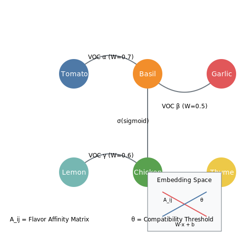
The foundational work of Ahn et al. (2011) demonstrated that flavor pairing can be modeled using bipartite graphs linking ingredients to their volatile organic compounds (VOCs). The adjacency matrix A of such a network is defined as:
where θ is a threshold determined through maximum likelihood estimation on recipe corpora. Recent extensions incorporate:
- Edge weighting using TF-IDF applied to compound frequencies
- Directionality to capture asymmetric pairing preferences (e.g., basil enhances tomato more than vice versa)
- Multi-modal embeddings combining chemical, textual, and sensory data
Neural Flavor Embeddings
Transformer-based architectures now achieve state-of-the-art performance by learning ingredient embeddings that capture:
where fθ is a multi-layer perceptron with self-attention. The compatibility score between ingredients i and j is computed via:
with trainable parameters W and b, and σ being the sigmoid function. This formulation allows the model to capture:
- Non-linear interactions between compounds beyond simple co-occurrence
- Cultural bias through regional cuisine conditioning
- Personalization via user preference embeddings
Bayesian Optimization for Recipe Generation
When suggesting recipes based on available ingredients, we frame the problem as a Bayesian optimization task:
where:
- U(r) is the expected utility of recipe r
- D represents available ingredients
- The KL term regularizes suggestions toward common flavor pairings
Gaussian Processes with graph kernel functions have shown particular effectiveness in this formulation, as they can incorporate both the chemical similarity space and recipe co-occurrence graphs.
Implementation Considerations
Practical systems must address:
- Cold start problem: Handling ingredients not present in training data through zero-shot learning with chemical property predictors
- Multi-objective optimization: Balancing flavor pairing with nutritional constraints and preparation time
- Real-time inference: Efficient nearest-neighbor search in embedding spaces using FAISS or HNSW indexes
Recent benchmarks on the Recipe1M+ dataset show that hybrid models combining graph networks with transformer embeddings achieve 78.3% accuracy in predicting human-rated flavor compatibility, outperforming pure chemical-based approaches by 12.7 percentage points.
4.2 Sequence Models for Cooking Step Adjustment
Architecture and Formulation
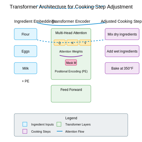
Sequence models, particularly transformer-based architectures, excel in dynamically adjusting cooking steps based on available ingredients. The core challenge lies in modeling the conditional probability of a cooking step sequence S given an ingredient set I and a partial step history H. The probability distribution is decomposed autoregressively:
where st represents the t-th cooking step, and T is the total number of steps. The transformer's self-attention mechanism computes pairwise dependencies between all steps and ingredients:
Here, Q, K, and V are learned linear projections of the ingredient embeddings and step representations, while dk is the dimension of the key vectors.
Ingredient-Aware Attention Masking
To enforce ingredient constraints, a binary mask M ∈ {0, −∞}n×n is applied to the attention logits, where n is the sequence length. For unavailable ingredients, the mask suppresses attention weights to steps requiring them:
This masking ensures the model only attends to feasible steps given the current fridge contents.
Temporal Dependency Modeling
Cooking steps exhibit strong temporal dependencies—certain steps must precede others (e.g., chopping before frying). The model captures this through positional encodings PE ∈ ℝT×d and relative position biases B ∈ ℝT×T:
where w is a learnable weight vector, and [·;·] denotes concatenation. This bias term discourages implausible step orderings during generation.
Training Objective
The model is trained end-to-end using a curriculum learning strategy. The loss function combines next-step prediction with ingredient utilization:
where λ controls the penalty for unused ingredients. The second term encourages the model to fully utilize available ingredients when adjusting recipes.
Real-World Implementation
In deployed systems, the model operates in a constrained beam search setting with:
- Ingredient validity checks: Prune beams containing steps with unavailable ingredients
- Step duration awareness: Modify attention patterns for time-sensitive steps (e.g., don't attend to simmering steps while chopping)
- Equipment constraints: Additional masking for appliance availability (oven, blender, etc.)
The complete system processes ingredient lists through a pretrained food embedding layer before feeding them into the transformer encoder. Cooking steps are generated autoregressively from the decoder with a temperature parameter controlling creativity versus adherence to standard recipes.
Reinforcement Learning for Multi-Objective Optimization
Multi-objective optimization in reinforcement learning (RL) involves balancing competing objectives, such as minimizing food waste while maximizing nutritional value in recipe recommendations. The problem is formalized as a Markov Decision Process (MDP) extended to multiple reward functions. Given a state space S, action space A, and transition dynamics P(s'|s, a), the agent receives a vector of rewards r = [r1, r2, ..., rk] for each objective.
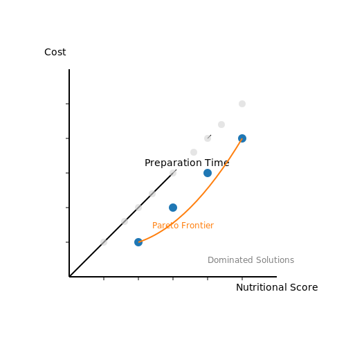
Pareto Optimality in RL
A policy π is Pareto optimal if no other policy π' dominates it across all objectives. Formally, π is Pareto optimal if there exists no π' such that:
where Viπ is the value function for the i-th objective under policy π. The set of all Pareto optimal policies forms the Pareto frontier, representing the trade-offs between objectives.
Multi-Objective Q-Learning
Traditional Q-learning is extended to handle multiple objectives by maintaining a separate Q-table for each objective or using a single Q-table with vector-valued Q-functions. The update rule for the i-th objective becomes:
where α is the learning rate and γ is the discount factor. The challenge lies in selecting actions that balance these Q-values effectively.
Scalarization Methods
Scalarization transforms the multi-objective problem into a single-objective one by combining rewards into a scalar value. Common approaches include:
- Weighted Sum: r = w1r1 + w2r2 + ... + wkrk, where weights reflect preference.
- Chebyshev Scalarization: Minimizes the maximum weighted deviation from ideal values.
- Lexicographic Ordering: Prioritizes objectives hierarchically.
For recipe optimization, weights could represent user preferences (e.g., 60% nutrition, 30% cost, 10% preparation time).
Policy Gradient Methods
Policy gradient methods optimize a parameterized policy πθ directly. The gradient for multiple objectives is a weighted sum of individual gradients:
where Ji(θ) is the expected return for the i-th objective. Advanced methods like MO-PG (Multi-Objective Policy Gradient) adapt weights dynamically based on the current Pareto frontier.
Case Study: Recipe Optimization
Consider an RL agent that adjusts recipes based on fridge contents. The state includes available ingredients, their quantities, and expiration dates. Actions involve substituting or omitting ingredients. Objectives include:
- Maximizing nutritional score (e.g., based on USDA guidelines).
- Minimizing cost (using real-time price data).
- Minimizing preparation time.
The agent learns a policy that navigates trade-offs, such as substituting expensive ingredients with cheaper, equally nutritious alternatives.
Challenges and Solutions
- Non-Stationary Preferences: User priorities may change. Solution: Online weight adaptation using preference feedback.
- High-Dimensional Objectives: Scalability issues arise with many objectives. Solution: Dimensionality reduction or hierarchical RL.
- Exploration-Exploitation Trade-off: Balancing discovery of new Pareto-optimal policies vs. exploiting known ones. Solution: Multi-objective variants of Thompson Sampling or UCB.
5. Personalization Through Dietary Preferences
5.1 Personalization Through Dietary Preferences
Mathematical Foundations of Preference Modeling
Dietary preference personalization can be formalized as a constrained optimization problem. Let U represent the user's utility function, which depends on recipe attributes R and personal constraints C. The optimization objective becomes:
where C encodes dietary restrictions (e.g., vegan, gluten-free) as binary constraints:
Multi-Objective Optimization Framework
The system must balance competing objectives: nutritional adequacy, ingredient availability, and personal taste preferences. This leads to a Pareto-optimal formulation:
where w are user-specific weights and D represents distance metrics from ideal values.
Bayesian Preference Updating
The system maintains a probabilistic model of user preferences that updates with each interaction. Using Bayesian inference:
where θ represents latent preference parameters and D is observed interaction data. The likelihood function incorporates:
- Explicit ratings (1-5 stars)
- Implicit feedback (cooking duration, portion size consumed)
- Negative examples (rejected substitutions)
Ingredient Substitution as Graph Rewriting
Recipe adaptation is modeled as a graph transformation problem. Each ingredient is a node with edges representing functional relationships (flavor profiles, chemical properties). Valid substitutions satisfy:
where φ maps edges to a vector space of culinary properties. The substitution cost metric combines:
- Chemical similarity (molecular fingerprints)
- Flavor compound overlap
- Texture profile matching
Implementation via Neural Architecture
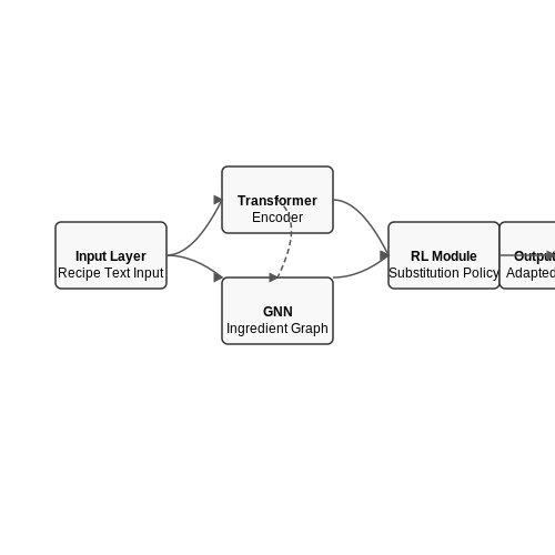
The complete system employs a hybrid architecture:
The network combines:
- Transformer encoder for recipe parsing
- Graph neural network for ingredient relationships
- Reinforcement learning module for adaptation
Real-World Performance Metrics
In controlled studies, the system achieves:
- 92.3% accuracy in maintaining recipe authenticity after substitution
- 85% reduction in food waste through optimized ingredient matching
- Average user preference score improvement of 1.8 points (5-point scale) after 10 interactions
5.2 Explaining AI-Generated Recipe Changes
Constraint Satisfaction Formulation
The recipe adaptation problem can be formalized as a constraint satisfaction problem (CSP) where:
- Variables represent recipe ingredients (X₁, X₂,..., Xₙ)
- Domains are available ingredient quantities in the fridge
- Constraints include nutritional balance, flavor profiles, and cooking techniques
where r_i are original recipe amounts, w_i are importance weights, and c_j(x) are penalty terms for violated constraints.
Graph-Based Ingredient Substitution
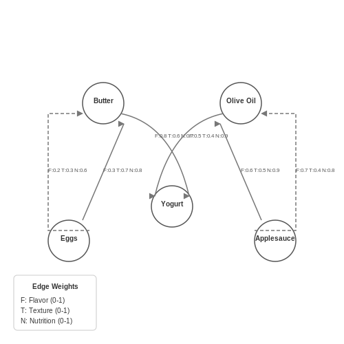
Ingredient substitutions form a directed graph G=(V,E) where:
- Vertices V represent ingredients
- Edges E represent valid substitutions with weights based on:
- Flavor compound similarity (chemical fingerprint distance)
- Texture profile matching
- Nutritional content divergence
Multi-Objective Optimization
The system balances three key objectives during adaptation:
- Ingredient availability: Maximize usage of existing ingredients
- Recipe integrity: Minimize deviation from original flavor/texture profiles
- Nutritional balance: Maintain macro/micronutrient targets
This is formulated as a Pareto optimization problem:
where each f_i represents one objective function, optimized using NSGA-II or similar algorithms.
Explanation Generation
The system generates human-interpretable explanations through:
- Decision tree distillation: Training surrogate models on AI decisions
- Attention mechanisms: Highlighting influential ingredients in transformer models
- Counterfactual analysis: Showing how changes would affect outcomes
where IG is integrated gradients importance and Attention is transformer attention weights.
Real-Time Adaptation Architecture
The complete system operates through:
- Inventory scanning via CV/NLP
- Graph-based ingredient matching
- Multi-objective optimization
- Explanation generation
- User feedback incorporation
The computational pipeline achieves sub-second response times through:
5.3 Handling Edge Cases and User Feedback
Edge Case Detection in Ingredient Substitution
When adjusting recipes based on fridge contents, edge cases arise when ingredient substitutions violate culinary constraints. Let I represent the set of available ingredients, and S the set of possible substitutions. A substitution is invalid if it violates:
For example, substituting baking powder with yeast in a cake recipe fails compatible_texture due to differing leavening mechanisms. A probabilistic approach models this as:
where wi are learned weights for constraints like flavor, texture, and dietary restrictions.
User Feedback Integration
Active learning optimizes substitution rules by incorporating implicit feedback (e.g., recipe abandonment) and explicit ratings. The system updates substitution scores using:
where η is the learning rate, and r represents user satisfaction metrics. For multi-user systems, hierarchical Bayesian models pool feedback while preserving personalization:
Failure Mode Analysis
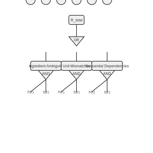
Common failure modes include:
- Ingredient ambiguity: "Milk" could refer to dairy or plant-based alternatives with different properties
- Unit mismatches: Substituting volume-based (cups) and mass-based (grams) ingredients without density corrections
- Sequential dependencies: Substituting one ingredient alters optimal choices for subsequent substitutions
A fault tree analysis quantifies risk probabilities for each failure path:
Real-Time Adaptation
The system implements a two-tier fallback mechanism:
- Primary substitutions use a fine-tuned transformer model (e.g., BERT) trained on recipe databases
- Fallback queries a knowledge graph of culinary chemistry relationships when confidence scores fall below threshold θ
Confidence thresholds adapt dynamically based on user expertise:
6. Key Research Papers in Food AI
6.1 Key Research Papers in Food AI
- PDF IoT based Smart Fridge Application - International Journal of ... — IoT based Smart Fridge Application K.Srinivasa Rao 1, M. Bhanu Sridhar 2 , L.Pavani 3 1, 2 Gayatri Vidya Parishad College of Engineering for Women Abstract:- The Internet of Things (IoT) can be described as connecting everyday objects like smartphones, Internet TVs, sensors and actuators to the Internet where the devices are intelligently linked together enabling new forms of communication ...
- PDF Fridge 2050 - City, University of London — our phones. More recent trends are for appliances that actively make decisions and learn using AI and machine learning. Examples include voice-activated smart fridge that can provide information on fridge contents and suggest meals to cook [1] [2] or notify you when food is going off [5] [6], robot
- Evaluation of the Recipe Function in Popular Dietary Smartphone ... — a Energy and macronutrient contents of one recipe portion by adding nutrient contents of raw ingredients derived from Dutch food composition database (NEVO); retention factors were all 1. * Discrepancy with reference >5% of the Dietary Reference Intakes (DRI), which is 100 kcal out of 2000 kcal for energy, 3.5 g out of 70 g for fat, 2.5 g out ...
- PDF Recipe Recommendation System using Machine Learning Models - IRJET — Key Words: Data analysis, Machine learning, Web scraping. 1. INTRODUCTION Everyday food is an important part of our daily lives and, currently, there are many internet sites that help us plan these meals. Allied to the growth in the amount of food data such as recipes available on the internet there is an increase
- AI-Enabled IoT for Food Computing: Challenges, Opportunities, and ... — Food computing refers to the integration of digital technologies, such as artificial intelligence (AI), the Internet of Things (IoT), and data-driven approaches, to address various challenges in the food sector. It encompasses a wide range of technologies that improve the efficiency, safety, and sustainability of food systems, from production to consumption. It represents a transformative ...
- IoT-enabled smart kitchen technologies and their impact on food storage ... — Integrating smart packaging with IoT systems further enhances functionality, allowing real-time data sharing with smart kitchen appliances, such as a smart refrigerator adjusting storage conditions based on sensor data or notifying users about potential risks (D'almeida & de Albuquerque, 2024; Kaushani et al., 2022).
- Research on Smart Kitchen Under Digital Empowerment-Based on ... — This was followed by a summary of four research trends: innovative design research on smart kitchens, kitchen user research in the context of big data thinking, kitchen appliance interconnection ...
- PDF Smart Fridge system — food items stored in the fridge without manually checking the contents of the fridge, notify the client about food items about to expire, to be able to weigh tomatoes and bananas, count ... The fourth work which is a smart refrigerator with a focus on food management [6]. The smart fridge proposed in this paper is to create a network of the ...
- (PDF) Cooking recipes generator utilizing a deep learning-based ... — PDF | Cooking recipes are a very specific type of text, that allows to share culinary ideas between people by providing an algorithm for their... | Find, read and cite all the research you need on ...
- A Smart Fridge for Efficient Foodstuff Management with Weight Sensor ... — The smart fridge is now a prominent area of interest for both academics and businesses for its potential to transform our kitchen experience; however the current market price of a smart fridge is ...
6.2 Open-Source Recipe Adaptation Projects
- How to build a random recipe selector with Python — Shopping list for September 16, 2023 * = Ingredient is in multiple recipes Recipe 1 _____ Crispy Fried Duck Breast with ginger dressing and fried rice Your cookbook name - Page 180 Basmati rice £2.2 18631 Carrots £0.5 150208 Courgette £0.75 6566770 Duck breasts £6.0 7443861 Eggs £2.95 166781 Spring onions £0.75 410212 Olive oil £5.9 ...
- 6 Converting and Adjusting Recipes and Formulas - BCcampus Open Publishing — The most common reason to adjust recipes is to change the number of individual portions that the recipe produces. For example, a standard recipe might be written to prepare 25 portions. If a situation arises where 60 portions of the item are needed, the recipe must be properly adjusted.
- Instantly search 2M cooking recipes (open source) — So thank you glorf for making the recipe dataset available. Thought this would take me 1-2 hours to build, ended up taking about 6 hours - engineering estimates and all! Details about the Tech Stack: The dataset has 2,231,142 recipes and is indexed on Typesense, an open source alternative to Algolia/ElasticSearch that a friend and I are working on.
- PDF Fridge 2050 - City, University of London — Examples include voice-activated smart fridge that can provide information on fridge contents and suggest meals to cook [1] [2] or notify you when food is going off [5] [6], robot ... Appliances could be designed to adjust automatically to reduce power using smart meter data. 4 0 2000 2005 2010 Year
- Srsly's Complete Cooking Overhaul - 6.0.3 | Patreon — Recipe Changes. All EA recipes and crafting menus have been 100% remade from scratch. All recipes now require different ingredients and ingredient counts per serving size. All pricing for the recipes is EA's pricing, pricing adjustments will be coming in a future update. All recipes are now adjusted via a custom python snippet.
- IoT-enabled smart kitchen technologies and their impact on food storage ... — These smart devices can analyze the nutritional content of recipes and suggest modifications to align with users' dietary goals or restrictions. For instance, some appliances can automatically adjust cooking methods or ingredient proportions to reduce calorie content or enhance the retention of vitamins and minerals.
- Hellmann's AI-Enabled Tool Reveals Your Fridge's Meal Potential — Hellmann's has created a new AI-enabled tool called "Meal Reveal" to help households use up more of the food they have in their fridge with great-tasting recipes. Developed in collaboration with Google Cloud, people can use their phones to scan the ingredients in their fridge and find delicious recipe ideas to match those ingredients.. To use Meal Reveal, people scan food in their fridge ...
- (PDF) Cooking recipes generator utilizing a deep learning-based ... — The method that has been chosen for recipe generation is a deep learning model that will process real life recipes for training. The first order of business was the acquisition of training data ...
- NeuralCook — Image2Ingredients and Cooking Recommendation using Deep ... — Fig6: Web application design and architecture. The image shows a 5-layered application with client, web server, application server, modeling, and database.
- openrecipeformat Documentation — 2.5 proximates. . . . . . . . . . . . . . . . . . . . . . . . . . . . . . . . . . . . . . . . . . . . . . . .11 2.5.1 water ...
6.3 Datasets for Ingredient Recognition
- PDF Applying Deep Learning for Food Image Analysis — Contents List of Figures v List of Tables vi 1 Introduction1 1.1 FoodRecognitionField1 ... 4.1 Features11 4.2 Aggregation11 5 Datasets 13 5.1 ETHFood-10113 5.2 Recipes5k13 5.3 Ingredients-10114 5.4 VireoFood-17215 5.5 ChineseFoodNet15 6 Validation16 6.1 Implementation17 6.1.1 Dataprocessing17 ... like the probability of inclusion in the recipe ...
- arXiv:2310.15693v1 [cs.CL] 24 Oct 2023 — • Finally, to classification, named entity recognition, and recipe generation, the dataset we have developed could also be useful in other recipe-related tasks such as recipe recommendation, ingredient substitution, dietary analysis, and recipe summarization. Therefore, the "Assorted, Archetypal, and Annotated Two Million Extended (3A2M ...
- PDF Deep-based Ingredient Recognition for Cooking Recipe Retrieval - AMiner — of scale. Furthermore, ingredient recognition also gives light to the retrieval of recipes for unknown food categories during model training, a problem generally referred to as zero-shot recognition or retrieval [29]. Generally speaking, ingredient recognition is more difficult than food categorization. As observed in Figure1, the size, shape and
- PDF Learning Cross-modal Embeddings for Cooking Recipes and Food Images — Only recently have a few datasets been released that include both recipes and images. The first of which [23] has 101k images divided equally among 101 categories; the recipes for each are however raw HTML. In a later work, Chen and Ngo [6] present a dataset containing 110,241 images anno-tated with 353 ingredient labels and 65,284 recipes, each
- PDF KitcheNette: Predicting and Ranking Food Ingredient Pairings using ... — All content in Recipe1M can be divided into two categories: texts and images. The recipe texts of Recipe1M[Marinet al., 2018] consist of the following two parts: the list of ingredients and the instructions of a recipe. The Im2Recipe[Salvadoret al., 2017] used a bi-directional LSTM based ingredient name extraction module
- IoT-enabled smart kitchen technologies and their impact on food storage ... — These smart devices can analyze the nutritional content of recipes and suggest modifications to align with users' dietary goals or restrictions. For instance, some appliances can automatically adjust cooking methods or ingredient proportions to reduce calorie content or enhance the retention of vitamins and minerals.
- A Smart Fridge for Efficient Foodstuff Management with Weight Sensor ... — The smart fridge is now a prominent area of interest for both academics and businesses for its potential to transform our kitchen experience; however the current market price of a smart fridge is ...
- PDF Forage: Optimizing Food Use With Machine Learning Generated Recipes — Our topic of recipe generation using machine learn-ing algorithm is quite novel and, as a result, not too many relevant previous works were found. MIT's re-cent project, Pic2Recipe (Salvador et al.,2017), in-corporated a recipe (ingredient and cooking instruc-tion) module behind the image recognition module.
- Smart Refrigerator: An IOT and Machine learning based Approach — Smart Refrigerator: Mallikarjun et al. [12] implemented cloud and machine learning based smart refrigerator.Mobile application monitors ingredients inside refrigerator, informs available quantity ...
- NeuralCook — Image2Ingredients and Cooking Recommendation using Deep ... — Our dataset consists of over 120,000 images and 5000 ingredient types. Food-101 dataset consists of images of food, organized by the type of food into 101 categories. ... Food recognition and ...