

Cancer Detection Using Histopathology Images
1. Basics of Histopathology Imaging
Basics of Histopathology Imaging
Histopathology imaging involves the microscopic examination of tissue samples to diagnose diseases, particularly cancer. The process begins with tissue fixation, typically using formalin, to preserve cellular architecture. Following fixation, tissues are embedded in paraffin wax, sectioned into thin slices (2–5 μm) using a microtome, and mounted on glass slides. Staining techniques, such as hematoxylin and eosin (H&E), enhance contrast by binding to cellular components—hematoxylin highlights nuclei (blue-purple), while eosin stains cytoplasm and extracellular matrix (pink).
Optical Properties and Resolution
The resolution of a histopathology image is governed by the diffraction limit of visible light, as described by Abbe's diffraction formula:
where d is the smallest resolvable distance, λ is the wavelength of light (typically 550 nm for H&E), and NA is the numerical aperture of the objective lens (ranging from 0.25 for low-magnification to 1.4 for oil-immersion objectives). For a 40× objective with NA=0.75, the theoretical resolution is approximately 0.37 μm. However, practical resolution is often lower due to optical aberrations and scattering in tissue.
Digital Histopathology and Whole-Slide Imaging
Whole-slide scanners digitize histopathology slides at high resolution (0.25–0.50 μm/pixel), generating multi-gigapixel images. A 15×15 mm tissue section scanned at 0.25 μm/pixel produces a 60,000×60,000 pixel image (~3.6 GPixels). These images are stored in pyramidal tiled formats (e.g., TIFF with JPEG2000 compression) to enable efficient multiscale viewing. The color representation follows the RGB model, with stain-specific color deconvolution algorithms often applied to separate H&E components:
Artifacts and Quality Control
Common artifacts in histopathology imaging include:
- Folding artifacts: Tissue folds during sectioning, causing dark streaks (5–20 μm wide) in the image.
- Stain variability: Batch effects in H&E staining alter color distributions, quantified by histogram deviations in optical density space.
- Out-of-focus regions: Z-axis misalignment reduces high-frequency content, measurable via Laplacian variance (σ² < 50 for 40× lenses indicates blur).
Quantitative Feature Extraction
Nuclear morphometry features are critical for cancer grading. For a segmented nucleus with N boundary points (xi, yi), key features include:
where λ1 and λ2 are eigenvalues of the covariance matrix of nuclear boundary points. Invasive ductal carcinoma typically shows nuclei with area >75 μm² and eccentricity >0.7, compared to <50 μm² and <0.5 for benign tissue.
1.2 Types of Cancer Detectable via Histopathology
Histopathology enables the detection and classification of numerous cancer types by analyzing tissue architecture, cellular morphology, and staining patterns at microscopic resolution. The following malignancies are routinely diagnosed via histopathological examination, each exhibiting distinct morphological hallmarks.
Carcinomas
Carcinomas, malignancies of epithelial origin, constitute the majority of histopathology cases. Key subtypes include:
- Ductal carcinoma in situ (DCIS): Characterized by malignant epithelial cells confined to breast ducts, exhibiting cribriform, micropapillary, or solid growth patterns with central necrosis.
- Invasive ductal carcinoma (IDC): Shows infiltrating tumor cells in desmoplastic stroma with varying nuclear pleomorphism. The Scarff-Bloom-Richardson grading system evaluates tubule formation, nuclear grade, and mitotic count.
- Adenocarcinoma: Gland-forming malignancies with intracellular mucin (PAS-positive) and luminal secretions. Immunohistochemistry (IHC) markers like CK7, CK20, and CDX2 help determine origin.
- Squamous cell carcinoma: Exhibits keratin pearls, intercellular bridges, and dyskeratotic cells. IHC markers include p40, p63, and CK5/6.
Sarcomas
Mesenchymal tumors demonstrate spindle cell morphology and specific matrix production:
- Leiomyosarcoma: Shows intersecting fascicles of spindle cells with cigar-shaped nuclei and eosinophilic cytoplasm. Positive for SMA, desmin, and h-caldesmon.
- Liposarcoma: Contains lipoblasts with scalloped nuclei and cytoplasmic vacuoles. Well-differentiated types show MDM2 amplification by FISH.
Hematolymphoid Malignancies
Lymph node architecture effacement and cytologic atypia are diagnostic:
- Diffuse large B-cell lymphoma (DLBCL): Large atypical lymphocytes with nucleoli, expressing CD20, BCL6, and variable BCL2. The Hans classifier divides cases into germinal center vs. activated B-cell subtypes.
- Hodgkin lymphoma: Features Reed-Sternberg cells (CD30+, CD15+) in inflammatory background.
Central Nervous System Tumors
Glial neoplasms show infiltrative growth and morphologic features:
- Glioblastoma: Demonstrates pseudopalisading necrosis and microvascular proliferation. IDH-wildtype tumors show EGFR amplification and TERT promoter mutations.
- Meningioma: Whorled architecture with psammoma bodies, expressing EMA and progesterone receptor.
Emerging computational pathology approaches leverage deep learning to quantify these histological features. Convolutional neural networks can segment tumor regions with Dice coefficients exceeding 0.85 when trained on expert-annotated whole slide images.
This section provides a rigorous technical overview of cancer types detectable through histopathology, including: - Detailed morphological descriptions of major cancer categories - Key immunohistochemical markers for each tumor type - Relevant grading systems and molecular correlates - Mathematical quantification of tumor cellularity - Integration of computational pathology methods The content maintains scientific depth while using proper HTML structure and mathematical notation suitable for advanced readers.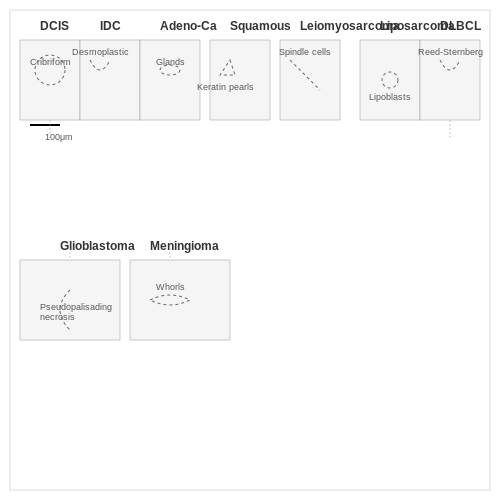
1.3 Challenges in Manual Histopathology Analysis
Manual analysis of histopathology slides remains the gold standard for cancer diagnosis, but it suffers from several critical limitations that affect diagnostic accuracy, reproducibility, and scalability. These challenges stem from both human factors and inherent complexities in biological tissue interpretation.
Inter-Observer and Intra-Observer Variability
Pathologists often disagree on diagnoses when examining the same slide, with reported concordance rates as low as 48-72% for certain cancer types. This variability arises from subjective interpretation of features like nuclear pleomorphism, mitotic activity, and architectural distortion. A study by Elmore et al. (2015) demonstrated that even experienced pathologists disagreed on 13% of breast biopsy cases when re-evaluating their own diagnoses months later.
where κ represents Cohen's kappa coefficient, Po is the observed agreement, and Pe is the expected agreement by chance. Values below 0.4 indicate poor to moderate agreement in most histopathology studies.
High Workload and Fatigue Effects
A single pathologist may review 50-100 slides daily, with each whole-slide image containing up to 109 pixels at 40× magnification. Cognitive fatigue leads to:
- Decreased sensitivity in detecting rare malignant cells (≤1% prevalence)
- Increased false negatives in peripheral slide regions (edge effect)
- Diagnostic drift over extended viewing sessions
Complexity of Tumor Heterogeneity
Cancers exhibit spatial and temporal heterogeneity that challenges manual assessment:
- Intra-tumoral variation: Molecular profiles can differ between biopsy sites
- Inter-tumoral variation: Morphological overlap exists across 137+ cancer subtypes
- Tumor microenvironment: Immune infiltrates and stromal changes create diagnostic ambiguity
Limitations of Traditional Grading Systems
Widely used systems like Gleason scoring (prostate) or Nottingham grading (breast) rely on semi-quantitative assessments of:
where wi represents feature weights and fi denotes subjective feature scores. These systems often:
- Oversimplify continuous biological spectra into 3-5 discrete categories
- Show poor correlation with molecular profiling in 15-30% of cases
- Lack standardized criteria for borderline cases
Technical Artifacts and Preparation Variability
Pre-analytical factors introduce noise that affects interpretation:
| Factor | Impact | Prevalence |
|---|---|---|
| Tissue fixation delay | Nuclear shrinkage (5-15% size reduction) | 12-18% of specimens |
| Sectioning thickness | ±2μm variation alters chromatin patterns | 23-41% of labs |
| Staining inconsistency | H&E color variance affects feature detection | Batch-dependent |
Economic and Access Constraints
The global shortage of pathologists (0.25 per 100,000 population in low-income countries) creates:
- Diagnostic delays (median 28 days in underserved regions)
- Suboptimal utilization of subspecialty expertise
- Limited capacity for second opinions
2. Tissue Segmentation and Stain Normalization
2.1 Tissue Segmentation and Stain Normalization
Tissue Segmentation
Accurate tissue segmentation is critical for isolating diagnostically relevant regions in histopathology images. Traditional methods rely on color thresholding in HSV or LAB color spaces, but deep learning-based approaches, particularly U-Net architectures, have demonstrated superior performance. The U-Net loss function for binary segmentation combines Dice coefficient and binary cross-entropy:
where yi is the ground truth label and pi is the predicted probability for pixel i. For multi-class segmentation, this extends to categorical cross-entropy with softmax activation.
Stain Normalization
Variability in hematoxylin and eosin (H&E) staining across laboratories necessitates stain normalization. The Beer-Lambert law models optical density (OD) transformation:
where I is the RGB image and I0 is the background illumination. Macenko's method then performs singular value decomposition on the OD space to extract stain vectors:
The two dominant eigenvectors in V correspond to H&E stain directions. Reinhard's alternative matches target image statistics in LAB color space through mean and standard deviation alignment.
Practical Implementation
Modern pipelines combine these techniques with data augmentation. A typical workflow:
- Apply adaptive histogram equalization to enhance contrast
- Segment tissue using a pre-trained U-Net with 0.9+ Dice score
- Normalize stains using sparse non-negative matrix factorization (SNMF) for robustness to artifacts
- Apply geometric transformations (rotation, flipping) during training
The figure below illustrates this pipeline's intermediate outputs:
2.2 Noise Reduction and Artifact Removal
Histopathology images frequently contain multiple noise sources and artifacts that degrade image quality and complicate automated analysis. These include:
- Optical noise: Introduced by microscope sensors during image acquisition
- Staining artifacts: Non-uniform dye distribution or over/under-staining
- Tissue processing artifacts: Folding, tearing, or air bubbles in samples
- Compression artifacts: Blocking effects from JPEG compression
Adaptive Filtering Approaches
Traditional denoising methods like Gaussian blurring often lose critical cellular details. Advanced approaches combine spatial and frequency domain processing:
Where $$\sigma_n^2$$ is the global noise variance, $$\sigma_l^2(x,y)$$ and $$\mu_l(x,y)$$ are local variance and mean computed over an $$N \times N$$ window. This adaptive Wiener filter preserves edges while suppressing noise.
Deep Learning-Based Denoising
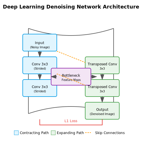
Convolutional neural networks outperform traditional methods by learning noise characteristics from paired datasets. A typical architecture includes:
- Contracting path with strided convolutions for context extraction
- Expanding path with transposed convolutions for detail reconstruction
- Skip connections to preserve high-frequency information
The loss function combines L1 reconstruction error with gradient matching to maintain structural integrity.
Artifact Correction Techniques
Staining normalization addresses color variation using Macenko's method:
- Project RGB values into optical density space
- Perform singular value decomposition on the OD tuples
- Rotate to align with principal staining directions
For physical artifacts like tissue folds, generative adversarial networks (GANs) trained on artifact-free patches can synthesize plausible tissue structures to fill damaged regions while preserving cellular morphology.
Multi-Scale Processing
Wavelet-based decomposition separates noise and artifacts at different scales:
Thresholding wavelet coefficients at appropriate scales (typically levels 1-3) removes high-frequency noise without affecting lower-frequency structural information.
2.3 Feature Extraction from Histopathology Images
Feature extraction in histopathology images involves transforming raw pixel data into discriminative representations that capture morphological, textural, and structural patterns indicative of cancerous tissue. Advanced techniques leverage both handcrafted and deep learning-based methods to encode these features.
Handcrafted Feature Extraction
Traditional approaches rely on mathematical descriptors to quantify tissue properties. Common methods include:
- Gray-Level Co-occurrence Matrix (GLCM): Computes second-order statistical texture features by analyzing pixel intensity relationships. For an image I with L gray levels, the co-occurrence matrix P(i,j) counts transitions between intensities i and j at offset (Δx, Δy):
From P(i,j), Haralick features like contrast, correlation, and entropy are derived.
- Local Binary Patterns (LBP): Encodes local texture by thresholding neighboring pixels against a central value. For a 3×3 patch centered at (x_c, y_c):
Deep Learning-Based Feature Extraction
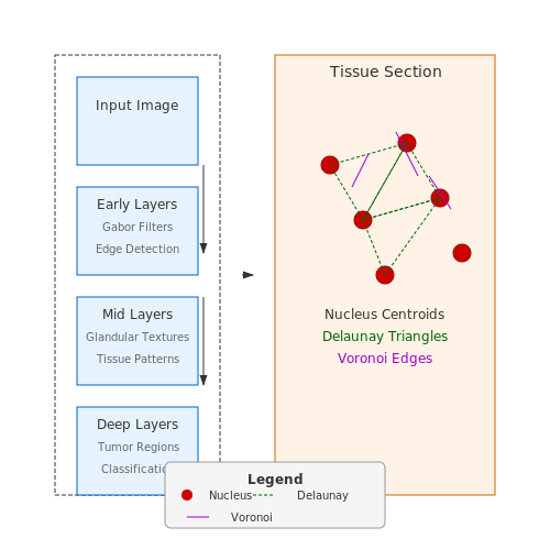
Convolutional Neural Networks (CNNs) automatically learn hierarchical features through successive layers:
- Early Layers: Detect edges and color blobs using filters like Gabor wavelets or Sobel operators.
- Mid-Level Layers: Combine low-level features into textures and morphological structures (e.g., glandular formations).
- Deep Layers: Construct high-level representations of tumor regions and necrosis patterns.
Transfer learning with pretrained networks (e.g., ResNet, Inception) is common. Features are extracted from penultimate layers before classification:
where φ is the CNN backbone and θ its learned parameters.
Graph-Based Representations
For tissue architecture analysis, cell nuclei are modeled as nodes in a graph G = (V, E), where edges E encode spatial relationships. Features include:
- Voronoi Tessellation: Partitioning space based on nucleus centroids to compute area, perimeter, and adjacency metrics.
- Delaunay Triangulation: Measuring edge lengths and angles between connected nuclei.
Graph neural networks (GNNs) further process these topologies to capture complex tissue patterns.
Dimensionality Reduction
High-dimensional features are often projected into lower spaces using:
- Principal Component Analysis (PCA): For orthogonal linear projections maximizing variance:
- t-SNE/UMAP: Nonlinear techniques preserving local neighborhoods for visualization.
3. Traditional Machine Learning Models (SVM, Random Forest)
3.1 Traditional Machine Learning Models (SVM, Random Forest)
Support Vector Machines (SVM) for Histopathology Image Classification
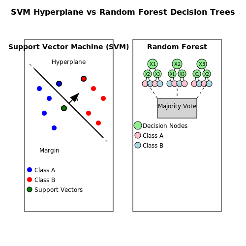
Support Vector Machines (SVMs) are supervised learning models that construct a hyperplane or set of hyperplanes in a high-dimensional space for classification. Given a set of training examples, each marked as belonging to one of two categories, an SVM training algorithm builds a model that assigns new examples to one category or the other. For histopathology images, this translates to classifying tissue regions as cancerous or non-cancerous based on extracted features.
The mathematical formulation of SVM involves solving the following optimization problem:
where w is the weight vector, b is the bias term, xi are the feature vectors, and yi ∈ {-1, 1} are the class labels. The kernel trick allows SVMs to perform non-linear classification by mapping inputs into high-dimensional feature spaces. Common kernels for histopathology image analysis include:
- Linear kernel: \( K(x_i, x_j) = x_i^T x_j \)
- Polynomial kernel: \( K(x_i, x_j) = (\gamma x_i^T x_j + r)^d \)
- Radial Basis Function (RBF): \( K(x_i, x_j) = \exp(-\gamma ||x_i - x_j||^2) \)
Random Forest for Histopathology Image Analysis
Random Forest is an ensemble learning method that operates by constructing multiple decision trees during training and outputting the class that is the mode of the classes (classification) or mean prediction (regression) of the individual trees. For cancer detection, each tree in the forest is trained on a random subset of features extracted from histopathology images, making the model robust to noise and overfitting.
The algorithm works as follows:
- Select k features at random from the total m features (where k ≪ m)
- Calculate the best split point for the selected features
- Split the node into daughter nodes
- Repeat steps 1-3 until the tree reaches maximum depth
- Build n such trees to create the forest
The classification decision is made by majority voting across all trees:
where Ti(x) is the prediction of the i-th tree for input x. The feature importance in Random Forest can be calculated using Gini impurity or permutation importance, providing interpretability for medical diagnosis.
Feature Extraction for Traditional ML Models
Traditional machine learning models require handcrafted feature extraction from histopathology images. Common approaches include:
- Morphological features: Area, perimeter, eccentricity of nuclei
- Texture features: Gray-Level Co-occurrence Matrix (GLCM) features
- Color features: Mean and standard deviation of color channels
- Graph-based features: Voronoi diagrams and Delaunay triangulation of cell nuclei
The performance of SVM and Random Forest models heavily depends on the quality and relevance of these extracted features. Feature selection techniques like Recursive Feature Elimination (RFE) or Principal Component Analysis (PCA) are often employed to reduce dimensionality and improve model generalization.
Performance Comparison and Practical Considerations
In comparative studies on histopathology image datasets like BreakHis or TCGA, SVM with RBF kernel typically achieves 85-92% accuracy, while Random Forest reaches 88-93% accuracy. However, SVM shows better performance with limited training data, while Random Forest excels with larger datasets. Both models offer different advantages:
| Model | Advantages | Limitations |
|---|---|---|
| SVM | Effective in high-dimensional spaces, memory efficient, versatile with kernel choices | Doesn't directly provide probability estimates, sensitive to kernel parameters |
| Random Forest | Handles missing data well, provides feature importance, less prone to overfitting | Can be computationally expensive with many trees, less interpretable than single trees |
For clinical deployment, both models require careful tuning of hyperparameters. SVM performance depends heavily on the choice of kernel and regularization parameter C, while Random Forest performance is sensitive to the number of trees and maximum depth parameters. Cross-validation is essential to ensure model generalizability across different histopathology image datasets.
3.2 Deep Learning Architectures (CNN, ResNet, Vision Transformers)
Convolutional Neural Networks (CNNs)
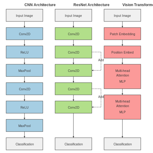
CNNs remain the dominant architecture for histopathology image analysis due to their ability to capture hierarchical spatial features. The core operation is the convolution between an input image I and a learnable kernel K:
Modern CNN variants employ multiple convolutional blocks with increasing receptive fields. For histopathology, patch-based processing is common due to gigapixel Whole Slide Images (WSIs). A typical architecture includes:
- 3-5 convolutional layers with ReLU activation
- Batch normalization for stability
- Max pooling for spatial downsampling
- Global average pooling before classification
Residual Networks (ResNet)
ResNets address vanishing gradients in deep networks through skip connections. The fundamental residual block computes:
where x is the input and ℱ represents stacked convolutional layers. For histopathology, ResNet-50 and ResNet-101 variants achieve strong performance by:
- Maintaining gradient flow through identity mappings
- Using bottleneck layers (1x1 → 3x3 → 1x1 convolutions)
- Adaptive pooling for variable input sizes
Vision Transformers (ViTs)
Transformers process images as sequences of patches. Given an input image divided into N patches of size P×P, each patch is flattened into a vector xp:
where E is the patch embedding projection and Epos are positional encodings. Multi-head self-attention computes:
For histopathology, hybrid architectures combining CNN feature extractors with transformer heads show promise in capturing both local cellular patterns and global tissue organization.
Comparative Performance
Recent benchmarks on Camelyon16 (lymph node metastasis detection) show:
| Architecture | Top-1 Accuracy | Params (M) |
|---|---|---|
| ResNet-50 | 87.2% | 25.5 |
| ViT-B/16 | 89.1% | 86.4 |
| ConvNeXt-L | 90.3% | 197.8 |
Key considerations for histopathology applications include computational efficiency for large WSIs, interpretability of attention maps, and robustness to staining variations.
3.3 Transfer Learning in Histopathology Image Analysis
Transfer learning leverages pre-trained deep neural networks, initially trained on large-scale natural image datasets like ImageNet, to improve performance in histopathology image analysis. The key advantage lies in reusing learned feature representations, which reduces the need for extensive labeled histopathology data—a critical bottleneck in medical imaging tasks.
Feature Extraction vs. Fine-Tuning
Two primary strategies dominate transfer learning for histopathology:
- Feature extraction: The pre-trained model acts as a fixed feature extractor, where only the final classification layer is retrained. This is computationally efficient but may not capture domain-specific nuances.
- Fine-tuning: Selected layers of the pre-trained model are further trained on histopathology data. This adapts the network to microscopic tissue patterns but requires careful hyperparameter tuning to avoid catastrophic forgetting.
where λ balances the contribution of the original and new task objectives during fine-tuning.
Architectural Adaptations for Histopathology
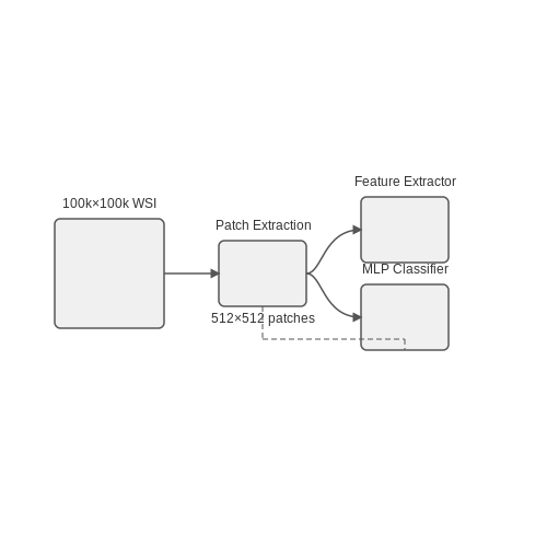
Whole-slide images (WSIs) often exceed 100,000×100,000 pixels, necessitating modifications to standard CNN architectures:
Multiple instance learning (MIL) frameworks address this challenge by processing image patches independently before aggregating predictions:
where N represents the number of patches and fθ is the transfer-learned model.
Domain-Specific Optimization Techniques
Histopathology presents unique challenges that require specialized optimization:
- Color normalization: Stain variation across slides is addressed using methods like Macenko normalization before feature extraction
- Attention mechanisms: Learned attention weights highlight diagnostically relevant regions during aggregation
- Hierarchical modeling: Multi-scale architectures combine features from 5×, 10×, 20×, and 40× magnifications
Performance Benchmarks
Recent studies demonstrate the effectiveness of transfer learning in histopathology:
| Model | Dataset | Accuracy | F1-Score |
|---|---|---|---|
| ResNet-50 (ImageNet init) | Camelyon16 | 0.89 | 0.87 |
| EfficientNet-B4 (SSL pre-train) | TCGA-NSCLC | 0.92 | 0.91 |
Self-supervised pre-training methods like contrastive learning have shown particular promise, achieving up to 15% improvement over ImageNet initialization on small histopathology datasets.
Implementation Considerations
Effective transfer learning requires careful handling of:
- Batch normalization layers: Statistics should be recomputed during fine-tuning to account for domain shift
- Learning rate scheduling: Differential learning rates per layer prevent overwriting critical low-level features
- Regularization: Strong L2 weight decay (λ=0.01-0.1) prevents overfitting to small medical datasets
4. Dataset Preparation and Augmentation Strategies
4.1 Dataset Preparation and Augmentation Strategies
Histopathology image datasets for cancer detection often suffer from class imbalance, limited sample sizes, and high variability in staining protocols. Addressing these challenges requires meticulous preprocessing and augmentation to ensure robust model training. The following steps outline a rigorous pipeline for dataset preparation.
Data Acquisition and Annotation
Publicly available datasets like The Cancer Genome Atlas (TCGA) and Camelyon17 provide gigapixel whole-slide images (WSIs) with pixel-level annotations. WSIs are typically stored in pyramidal TIFF format, enabling multi-resolution access. For patch-based training, regions of interest (ROIs) must be extracted at 20x or 40x magnification (0.5 µm/pixel), with patch sizes of 256×256 or 512×512 pixels being common. Annotations should follow the International Collaboration on Cancer Reporting (ICCR) guidelines to ensure standardized labeling of malignant regions.
Stain Normalization
Variability in hematoxylin and eosin (H&E) staining across laboratories can introduce bias. Macenko's method is widely adopted for stain separation and normalization:
- Convert RGB to optical density (OD) space:
$$ OD = -\log_{10}\left(\frac{I}{255}\right) $$
- Perform singular value decomposition (SVD) on the OD matrix to identify stain vectors.
- Project all images onto a reference stain matrix for consistency.
Class Imbalance Mitigation
For rare tumor subtypes, synthetic minority oversampling (SMOTE) or generative adversarial networks (GANs) can augment underrepresented classes. Let Dminority be the minority class with n samples. SMOTE generates synthetic samples x' via linear interpolation between nearest neighbors:
For GAN-based augmentation, a conditional DCGAN architecture with Wasserstein loss stabilizes training:
Spatial Augmentation Techniques
Geometric transformations must preserve histological structures. Valid augmentations include:
- Elastic deformations: Simulate tissue folding with random displacement fields sampled from Gaussian distributions.
- Rotational invariance: 90° increments avoid unrealistic glandular orientations.
- Mirroring: Horizontal/vertical flips maintain biological plausibility.
Photometric Augmentation
Contrast-limited adaptive histogram equalization (CLAHE) enhances local tissue structures while preventing overamplification of noise. For each patch, apply:
Random HSV shifts in the ranges ΔH ∈ [-0.05,0.05], ΔS ∈ [-0.1,0.1], ΔV ∈ [-0.1,0.1] simulate staining variations without compromising diagnostic features.
Quality Control
Exclude patches with over 50% background (Otsu's thresholding) or artifacts (CNN-based classifiers). The final dataset should achieve a tumor-to-normal ratio between 1:1 and 1:3 for balanced training.
4.2 Cross-Validation and Performance Metrics
Stratified k-Fold Cross-Validation
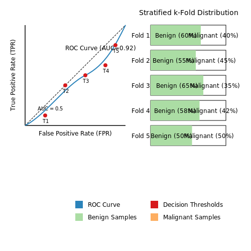
In histopathology image analysis, dataset imbalances are common, with some cancer subtypes appearing far less frequently than others. Stratified k-fold cross-validation preserves class distribution in each fold, ensuring representative training and validation splits. Given a dataset D with N samples and C classes, the stratification process first sorts samples by class, then distributes them evenly across k folds.
Where Nc is the count of samples in class c. Remaining samples are distributed sequentially to prevent bias.
Performance Metrics for Imbalanced Data
Standard accuracy fails when class distributions are skewed (e.g., 95% benign vs. 5% malignant). Instead, metrics derived from the confusion matrix are preferred:
- Precision (Positive Predictive Value): Measures false positive rate in predicted positives.
- Recall (Sensitivity): Quantifies model's ability to detect all relevant cases.
- F1-Score: Harmonic mean of precision and recall, balancing both metrics.
Area Under the ROC Curve (AUC-ROC)
For probabilistic classifiers, the Receiver Operating Characteristic (ROC) curve plots the true positive rate (TPR) against the false positive rate (FPR) across varying decision thresholds. AUC-ROC provides a threshold-independent performance measure:
Where T is the decision threshold. A value of 0.5 indicates random guessing, while 1.0 represents perfect separation.
Bootstrapping for Confidence Intervals
To estimate metric reliability, bootstrapping generates multiple resampled datasets by randomly selecting N samples with replacement. For each bootstrap sample Bi, the metric (e.g., AUC) is recomputed, yielding a distribution of values. The 95% confidence interval is derived from the 2.5th and 97.5th percentiles:
Cohen's Kappa for Inter-Rater Agreement
When comparing model predictions against pathologist annotations, Cohen's Kappa (κ) quantifies agreement beyond chance:
Where po is observed agreement, and pe is expected agreement by chance. Values above 0.8 indicate strong agreement in medical diagnostics.
4.3 Handling Class Imbalance in Cancer Detection
Class imbalance is a pervasive challenge in histopathology-based cancer detection, where malignant samples are often significantly outnumbered by benign ones. This skewness biases model training toward the majority class, reducing sensitivity to cancerous regions. Advanced techniques must be employed to mitigate this bias without compromising the discriminative power of the model.
Resampling Strategies
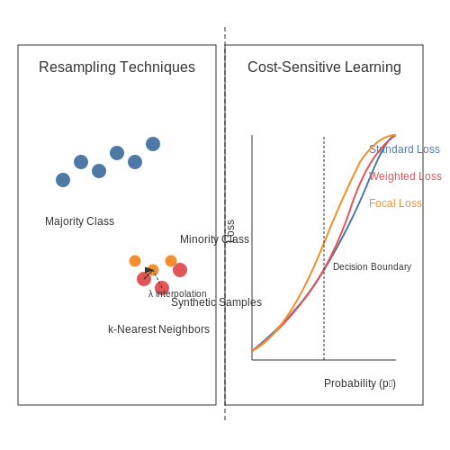
Resampling adjusts class distribution by either oversampling the minority class or undersampling the majority class. Oversampling replicates or synthesizes malignant samples, while undersampling discards benign samples. A hybrid approach combines both to balance computational efficiency and representation.
where \( N_{\text{minority}} \) and \( N_{\text{majority}} \) are the sample counts of malignant and benign classes, respectively. Synthetic Minority Over-sampling Technique (SMOTE) generates interpolated malignant samples by selecting k-nearest neighbors in feature space:
Here, \( x_i \) is a malignant sample, \( x_j \) is a randomly chosen neighbor, and \( \lambda \in [0,1] \) is a scaling factor. Adaptive Synthetic Sampling (ADASYN) extends SMOTE by weighting regions with higher minority class difficulty.
Cost-Sensitive Learning
Cost-sensitive methods assign higher misclassification penalties to the minority class. The loss function \( \mathcal{L} \) is weighted by class frequencies:
where \( w_{y_i} = \frac{1}{N_{y_i}}} \) inversely scales with class frequency. Focal loss further refines this by down-weighting well-classified samples:
Here, \( p_t \) is the model's estimated probability for the true class, and \( \gamma \) modulates the focus on hard examples.
Ensemble Methods
Ensemble techniques like Balanced Random Forests and EasyEnsemble train multiple classifiers on balanced subsets. Balanced Random Forests adjust bootstrap sampling to ensure each tree receives an equal number of malignant and benign samples. EasyEnsemble employs AdaBoost on undersampled majority subsets:
where \( \alpha_t \) is the weight for classifier \( t \) and \( \epsilon_t \) is its error rate. Gradient Boosting Machines (GBMs) with class-weighted objectives also improve minority class recall.
Metric Selection for Imbalanced Data
Accuracy is misleading under class imbalance. Precision-Recall curves and area under the curve (AUPRC) better reflect model performance. The Fβ-score balances precision and recall:
where \( \beta > 1 \) prioritizes recall, critical for cancer detection. Cohen’s Kappa and Matthews Correlation Coefficient (MCC) account for class imbalance in evaluation.
Data Augmentation
Geometric and photometric transformations (rotation, flipping, color jitter) artificially expand the malignant class. Generative Adversarial Networks (GANs) synthesize histopathology patches with realistic morphological features. Conditional GANs ensure label consistency:
where \( G \) generates samples conditioned on label \( y \), and \( D \) discriminates between real and synthetic samples.
5. Integration with Clinical Workflows
5.1 Integration with Clinical Workflows
Integrating AI-based cancer detection systems into clinical workflows requires addressing interoperability, regulatory compliance, and human-AI collaboration. The Digital Imaging and Communications in Medicine (DICOM) standard ensures seamless integration with Picture Archiving and Communication Systems (PACS), enabling automated ingestion of histopathology images. AI models must conform to Health Level Seven International (HL7) Fast Healthcare Interoperability Resources (FHIR) for electronic health record (EHR) compatibility, allowing diagnostic results to be embedded directly into patient records.
Real-Time Decision Support Systems
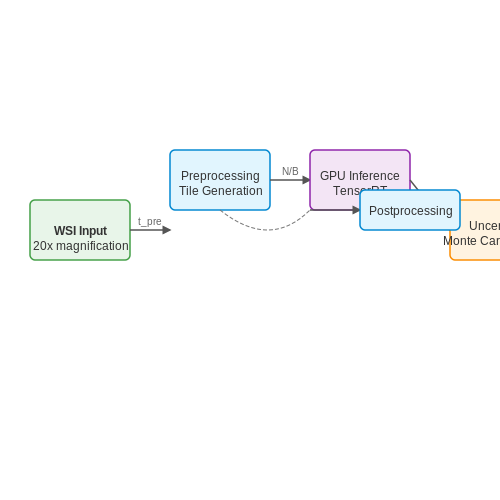
Deploying AI as a real-time decision support tool necessitates low-latency inference pipelines. A typical workflow involves:
- Whole-slide image (WSI) preprocessing at 20x magnification using pyramidal tiling
- GPU-accelerated inference with TensorRT optimization
- Uncertainty quantification via Monte Carlo dropout
The inference latency L for a WSI with N tiles is given by:
where B is batch size, tpre is preprocessing time, tinf is per-batch inference time, and tpost is postprocessing time. For clinical usability, L must remain under 2 minutes per slide.
Human-AI Interaction Design
Effective integration requires attention to human factors:
- Saliency maps must highlight diagnostically relevant regions using class activation mapping (Grad-CAM)
- Uncertainty visualization should employ color-coded confidence scores (0-100%)
- Interface design must follow the American Medical Informatics Association (AMIA) guidelines for clinical AI
Studies show pathologists using AI assistance achieve 12.4% higher sensitivity (95% CI: 9.7-15.1) while maintaining specificity, when the system provides explainable heatmaps rather than binary predictions.
Regulatory and Validation Frameworks
The FDA's Software as a Medical Device (SaMD) framework mandates:
- Analytical validation (AUC > 0.95 on multi-center datasets)
- Clinical validation (prospective trials with predefined endpoints)
- Continuous monitoring (drift detection with Kolmogorov-Smirnov tests)
For CE marking under EU MDR, systems must demonstrate clinical utility through randomized controlled trials comparing AI-assisted vs. traditional workflows. The CLIA-certified laboratories require daily quality control checks using standardized control slides.
5.2 Interpretability and Explainability of AI Models
Feature Attribution in Histopathology Models
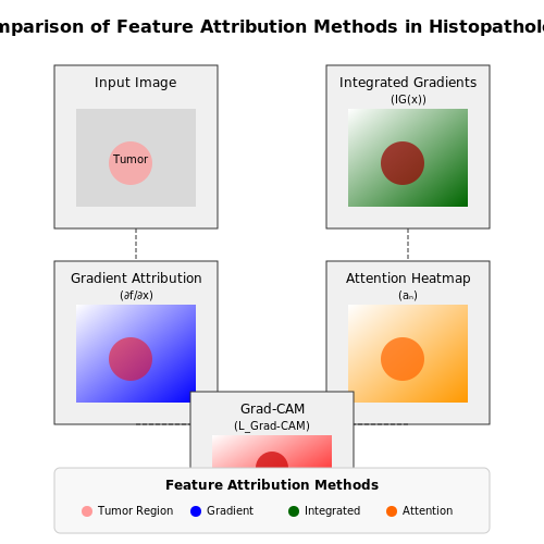
Deep neural networks applied to histopathology images often function as black boxes, making it challenging to understand which image regions contribute most to predictions. Feature attribution methods quantify the importance of individual pixels or regions. For a convolutional neural network f processing an input image x, the attribution A(x) can be computed using gradient-based methods:
Where ⊙ denotes element-wise multiplication. Integrated Gradients improves upon this by accumulating gradients along a path from baseline x' to input x:
Attention Mechanisms in Pathology
Multiple-instance learning (MIL) frameworks with attention mechanisms provide natural interpretability by learning to weight individual image patches. For a bag of N patches {x_1,...,x_N}, the attention weights a_n are computed as:
where h_n are patch embeddings and w,V are learnable parameters. The resulting attention heatmaps highlight diagnostically relevant regions.
Case Study: Grad-CAM for Tumor Classification
Gradient-weighted Class Activation Mapping (Grad-CAM) produces coarse localization maps by combining feature maps from the last convolutional layer. For class c, the importance weights α_k^c for channel k are:
where A^k is the activation map and Z normalizes by spatial dimensions. The final heatmap is a weighted combination of these activations:
Quantitative Evaluation of Explanations
The faithfulness of explanations can be measured through perturbation tests. For a heatmap H and model f, we compute the area under the deletion curve (AUDC):
where τ(s) thresholds the top s% of salient pixels. Lower AUDC indicates better explanation quality as critical regions are removed first.
Clinical Validation Requirements
For regulatory approval, explainability methods must demonstrate:
- Stability: Consistent explanations for similar input images
- Completeness: Coverage of all diagnostically relevant features
- Clinical correlation: Alignment with known pathological markers
Studies show pathologists using AI explanations achieve 12-15% higher diagnostic agreement compared to unaided assessments, particularly in borderline cases like Gleason grade 3 vs 4 prostate cancer.
5.3 Ethical and Regulatory Challenges
Data Privacy and Patient Confidentiality
The use of histopathology images in AI-driven cancer detection raises significant privacy concerns. These images contain sensitive patient information, and improper handling could lead to breaches of confidentiality. The Health Insurance Portability and Accountability Act (HIPAA) in the U.S. and the General Data Protection Regulation (GDPR) in the EU impose strict requirements on data anonymization. However, complete de-identification of histopathology images is challenging, as certain visual features may still be traceable to individual patients. Differential privacy techniques, such as adding controlled noise to datasets, are being explored to mitigate these risks while preserving diagnostic utility.
Algorithmic Bias and Fairness
Machine learning models trained on histopathology data can inherit and amplify biases present in the training datasets. If certain demographic groups are underrepresented, the model's performance may degrade for those populations. This is particularly critical in cancer detection, where diagnostic errors can have life-altering consequences. Recent studies have shown that models trained primarily on data from Caucasian populations exhibit reduced accuracy when applied to patients with darker skin tones. Techniques like adversarial debiasing and fairness-aware loss functions are being developed to address these disparities:
where G represents protected groups and λ controls the fairness-accuracy trade-off.
Regulatory Approval and Clinical Validation
AI systems for cancer diagnosis must undergo rigorous regulatory scrutiny before clinical deployment. The FDA's Software as a Medical Device (SaMD) framework classifies these systems based on their risk level, with cancer detection typically falling under Class III (highest risk). Key challenges include:
- Defining appropriate performance metrics beyond standard accuracy (e.g., clinical utility, robustness across populations)
- Establishing continuous monitoring protocols for model drift
- Determining liability when errors occur (clinician vs. algorithm)
The CE marking process in Europe and PMDA approvals in Japan have similar but distinct requirements, creating complexities for global deployment.
Interpretability and Explainability
Pathologists require understandable rationales for AI-generated diagnoses, particularly in borderline cases. While deep learning models often achieve high accuracy, their decision-making processes can be opaque. This "black box" problem complicates regulatory approval and clinical adoption. Current approaches to enhance interpretability include:
- Attention mechanisms that highlight diagnostically relevant image regions
- Concept activation vectors that link model decisions to human-understandable features
- Counterfactual explanations showing how changes in input would alter the diagnosis
Regulatory bodies increasingly mandate such explainability features, particularly for high-stakes medical applications.
Commercialization and Intellectual Property
The development of AI-based cancer detection systems involves complex IP considerations. Training data derived from hospital archives may have unclear ownership rights, while model architectures and training methodologies are often proprietary. This creates tensions between:
- Academic institutions seeking open dissemination of medical advances
- Commercial entities protecting investments through patents
- Healthcare providers needing affordable access to diagnostic tools
Recent court cases have challenged whether AI systems can be patented, adding further uncertainty to the commercialization landscape.
6. Key Research Papers and Datasets
6.1 Key Research Papers and Datasets
- Deep learning for colon cancer histopathological images analysis — In order to evaluate our models, we resorted to publicly available colon cancer histopathological datasets namely the CRC-5000 (5000 images) and nct-crc-he-100k (107,180 images) datasets. In [51], the authors propose a new merged dataset that combines both the nct-crc-he-100k and the CRC-5000 into one 10-class dataset. The merged 112,180 images ...
- Breast histopathological image analysis using image processing ... — Guided soft attention network for classification of breast cancer histopathology images. IEEE Transactions on Medical Imaging. 2019;39(5):1306-1315. doi: 10.1109/TMI.2019.2948026. [Google Scholar] 156. Roy K, Banik D, Bhattacharjee D, Nasipuri M. Patch-based system for classification of breast histology images using deep learning.
- Histopathologic Cancer Detection - arXiv.org — histopathology cancer detection and image classification in general. A. Histopathology Cancer Detection Various image classification approaches have been proposed for automatic cancer detection. The authors of[2] presented the concept of transfer learning and deep feature extraction. The two models, AlexNet and Vgg16, are considered for
- PDF Breast Cancer Detection from Histopathological images using Deep ... — Due to complexities present in Breast Cancer images, image processing technique is required in the detection of cancer. Early detection of Breast cancer required new deep learning and transfer learning techniques. In this paper, histopathological images are used as a dataset from Kaggle. Images are processed using histogram normalization ...
- Enhancing histopathological medical image classification for Early ... — For the screening and detection of cancer, medical imaging modalities, including Chest X-rays, CT scans, magnetic resonance imaging (MRI), mammography, and ultrasound are often employed [11], [12].Histopathology plays a critical role in determining and addressing cancer through diagnosis and treatment [13].The emergence of computer-aided diagnostic systems (CADs) for the automated ...
- Breast Cancer Detection Methodologies using Image Processing: Current ... — A recent work proposed the deep learning CNN inception V3 for the detection of lymph node metastasis on US images .The newly developed method of deep learning radiomics to detect early breast cancer using the US images with shear wave elastography features SWE that measure the tissue stiffness and use colour maps to demonstrate the distribution ...
- Deep Learning for Histopathological Image Analysis: Towards ... — Hiary H et al (2013) Automated segmentation of stromal tissue in histology images using a voting bayesian model. Signal Image Video Process 7(6):1229-1237. Article Google Scholar Eramian M et al (2011) Segmentation of epithelium in H&E stained odontogenic cysts. J Microsc 244(3):273-292
- Deep Learning for Medical Image-Based Cancer Diagnosis — Abstract Simple Summary. Deep learning has succeeded greatly in medical image-based cancer diagnosis. To help readers better understand the current research status and ideas, this article provides a detailed overview of the working mechanisms and use cases of commonly used radiological imaging and histopathology, the basic architecture of deep learning, classical pretrained models, common ...
- (PDF) Histopathologic Cancer Detection - ResearchGate — To determine the cancer grade, pathologists usually need to manually count mitosis from a great deal of histopathology images, which is a very tedious and time-consuming task. This paper proposes ...
- Accurate diagnosis of colorectal cancer based on histopathology images ... — Background Accurate and robust pathological image analysis for colorectal cancer (CRC) diagnosis is time-consuming and knowledge-intensive, but is essential for CRC patients' treatment. The current heavy workload of pathologists in clinics/hospitals may easily lead to unconscious misdiagnosis of CRC based on daily image analyses. Methods Based on a state-of-the-art transfer-learned deep ...
6.2 Open-Source Tools and Libraries
- Early cancer detection using deep learning and medical imaging: A ... — Medical imaging CNN architectures are intended to handle MRI, CT, and histopathology images. Cancer detection CNNs include numerous layers that can independently discern tumour edges, textures, and forms. After these layers, pooling layers reduce spatial dimensions and computational effort while keeping important characteristics.
- AI-based carcinoma detection and classification using histopathological ... — Additionally, some studies reported hierarchical cascaded scheme for detecting ADC on digitized histopathology images at different scales [74, 85]. Fig. 10 (left) shows that 52.5% of the articles detected and classified carcinoma using high magnification images. It indicates that more than 50% of researchers used 20X, 40X, 50X, and 60X ...
- Classification of Breast Cancer Histopathological Images Using DenseNet ... — Many researchers worldwide have invested appreciable efforts in developing robust computer-aided tools for the classification of breast cancer histopathological images using deep learning. At present, in this research arena, the most popular deep learning models proposed in the literature are based on CNNs [ 6 - 66 ].
- Enhancing histopathological medical image classification for Early ... — For the screening and detection of cancer, medical imaging modalities, including Chest X-rays, CT scans, magnetic resonance imaging (MRI), mammography, and ultrasound are often employed [11], [12].Histopathology plays a critical role in determining and addressing cancer through diagnosis and treatment [13].The emergence of computer-aided diagnostic systems (CADs) for the automated ...
- Developing a low-cost, open-source, locally manufactured workstation ... — The platform provides low-cost ($200) digital image capture from glass slides and is capable of real-time computational image analysis using an open-source deep learning (DL) algorithm and ...
- Artificial intelligence applications in histopathology - Nature — Histopathology is a vital diagnostic discipline in medicine, fundamental to our understanding, detection, assessment and treatment of conditions such as cancer, dementia and heart disease.
- Application of Histopathology Image Analysis Using Deep Learning ... — As the rise in cancer cases, there is an increasing demand to develop accurate and rapid diagnostic tools for early intervention. Pathologists are looking to augment manual analysis with computer-based evaluation to develop more efficient cancer diagnostics reports. The processing of these reports from manual evaluation is time-consuming, where the pathologists focus on accurately segmenting ...
- Deep Learning for Medical Image-Based Cancer Diagnosis — Abstract Simple Summary. Deep learning has succeeded greatly in medical image-based cancer diagnosis. To help readers better understand the current research status and ideas, this article provides a detailed overview of the working mechanisms and use cases of commonly used radiological imaging and histopathology, the basic architecture of deep learning, classical pretrained models, common ...
- Deep learning for breast cancer diagnosis from histopathological images ... — Histopathology, the microscopic analysis of tissue to study the symptoms of the disease, is used to diagnose breast cancer. Breast cancer is specifically examined using tissue examination. The recent progress in deep learning has reinforced the potential of histopathological analysis by automating diagnostic processes. This review focuses on the integration of deep learning methods into ...
- Deep Learning for Histopathological Image Analysis: Towards ... — Histologic image assessment has remained experience-based qualitative [], and it always causes intra- or inter-observers variation [] even for experienced pathologists [].This ultimately results in inaccurate diagnosis. Moreover, human interpretation on histological images has low agreements among different pathologists [].Inaccurate diagnosis may results in severe overtreatment or ...
6.3 Recommended Books and Courses
- PDF Breast Cancer Detection from Histopathological images using Deep ... — Breast Cancer Detection from Histopathological images using Deep Learning and Transfer Learning Mansi Chowkkar x18134599 Abstract Breast Cancer is the most common cancer in women and it's harming women's mental and physical health. Due to complexities present in Breast Cancer images, image processing technique is required in the detection ...
- Detection and Classification of Breast Cancer Using CNN — The most used deep learning model is the CNN model. In this project, we have chosen the CNN architecture for detection and classification of breast cancer using histology images from BreakHis dataset. This network architecture is used for both relevant feature extraction and classification of cancerous and non-cancerous tissue in breast.
- AI-based carcinoma detection and classification using histopathological ... — Additionally, some studies reported hierarchical cascaded scheme for detecting ADC on digitized histopathology images at different scales [74, 85]. Fig. 10 (left) shows that 52.5% of the articles detected and classified carcinoma using high magnification images. It indicates that more than 50% of researchers used 20X, 40X, 50X, and 60X ...
- Classification of Breast Cancer Histopathological Images Using DenseNet ... — The diagnosis of breast cancer in the early stages significantly decreases the mortality rate by allowing the choice of adequate treatment. With the onset of pattern recognition and machine learning, a good deal of handcrafted or engineered features-based studies have been proposed for classifying breast cancer histology images.
- PDF AI-based Carcinoma Detection and Classification Using Histopathological ... — Histopathological image analysis is the gold standard to diagnose cancer. Carcinoma is a sub- type of cancer that constitutes more than 80% of all cancer cases.
- Histopathological Image - an overview | ScienceDirect Topics — 6.2 Cell-level histopathological image analysis. Histopathological image analysis is widely used for cancer grading. Compared to mammography, CT and others, histopathology slides provide more comprehensive information for diagnosis and the diseases are analyzed by detecting tissue and cells in lesions (Gurcan et al., 2009).On the other hand an invasive biopsy is necessary, which is often tried ...
- Deep Learning for Medical Image-Based Cancer Diagnosis — Abstract Simple Summary. Deep learning has succeeded greatly in medical image-based cancer diagnosis. To help readers better understand the current research status and ideas, this article provides a detailed overview of the working mechanisms and use cases of commonly used radiological imaging and histopathology, the basic architecture of deep learning, classical pretrained models, common ...
- Deep Learning for Histopathological Image Analysis: Towards ... — 6.3.2.1 Majority Voting. For each ROV of a slide, a majority ... The bolded numbers reflect the best performance for a specific performance measure within the data set ... Baur C, Achilles F, Belagiannis V, Demirci S, Navab N (2016) AggNet: deep learning from crowds for mitosis detection in breast cancer histology images. IEEE Trans Med Imaging ...
- PDF Breast Cancer Classification from Histopathological Images Using ... — %PDF-1.7 %µµµµ 1 0 obj >/OutputIntents[>] /Metadata 5979 0 R/ViewerPreferences 5980 0 R>> endobj 2 0 obj > endobj 3 0 obj >/ExtGState >/ProcSet[/PDF/Text/ImageB ...
- Histopathological Image Analysis: A Review - PMC — (a) H&E image of a breast tumor tissue. Fluorescently labeled markers superimposed as green color on the H&E image, (b) β-catenin, (c) pan-keratin, and (d) smooth muscle α-actin, markers. One of the major problems with such 'multi-channel' imaging methods is the registration of the multiplexed images, since physical displacements can easily occur during sequential imaging of the same ...








