Dynamic Graph Neural Networks for Procedural Reasoning
1. Graph Neural Networks: Core Concepts and Architectures
Graph Neural Networks: Core Concepts and Architectures
Graph Representation Learning Fundamentals
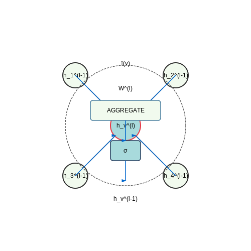
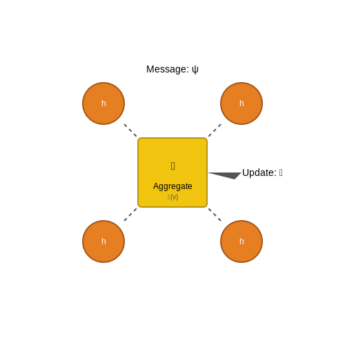
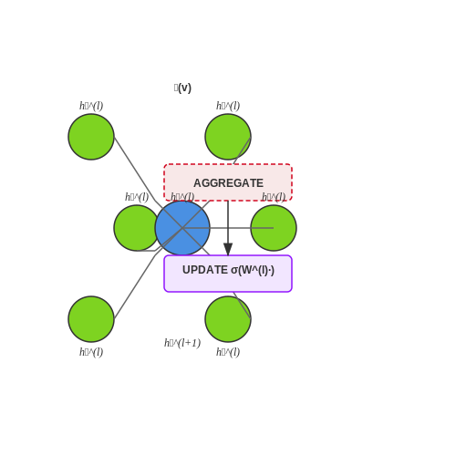
Graph Neural Networks (GNNs) operate on graph-structured data G = (V, E), where V represents nodes (vertices) and E denotes edges connecting these nodes. The fundamental operation in GNNs is message passing, where node representations are iteratively updated by aggregating information from neighboring nodes. For a node v at layer l, the update rule is:
where σ is a non-linear activation function, W(l) is a learnable weight matrix, and AGGREGATE is a permutation-invariant function (typically mean, sum, or max pooling). The neighborhood 𝒩(v) includes all nodes adjacent to v.
Spectral vs Spatial Approaches
GNN architectures bifurcate into spectral and spatial methods. Spectral approaches leverage graph Fourier transforms, operating in the spectral domain of the graph Laplacian L = D - A, where D is the degree matrix and A the adjacency matrix. The spectral convolution is defined as:
where U contains the eigenvectors of L, and gθ is a learnable filter in the spectral domain. In contrast, spatial methods directly operate on the graph structure by aggregating neighbor information, avoiding the computationally expensive eigendecomposition.
Key Architectural Variants
Graph Convolutional Networks (GCNs)
GCNs implement a first-order approximation of spectral convolutions using the normalized adjacency matrix  = D̃-½ÃD̃-½, where à = A + I adds self-loops. The layer-wise propagation rule is:
This formulation enables efficient batched operations while maintaining the theoretical connection to spectral graph theory.
Graph Attention Networks (GATs)
GATs introduce attention mechanisms to learn dynamic edge weights. The attention coefficients between node i and j are computed as:
where a is a learnable attention vector and || denotes concatenation. This allows the model to focus on the most relevant neighbors during aggregation.
Expressive Power and Theoretical Limits
The Weisfeiler-Lehman (WL) test provides a framework for analyzing GNN expressive power. A GNN's ability to distinguish non-isomorphic graphs is bounded by the 1-WL test. Modern architectures achieve greater expressivity through:
- Higher-order propagation rules (k-GNNs)
- Injecting random features or positional encodings
- Differentiable pooling operations (DiffPool)
The universal approximation capability of GNNs is formally established when the aggregation and update functions are injective, enabling distinct multisets of neighbor features to map to distinct node representations.
Handling Edge Dynamics
For procedural reasoning tasks, GNNs must adapt to evolving edge structures. Temporal Graph Networks (TGNs) address this by maintaining a memory module mi(t) for each node, updated through:
where Δt is the time since the last update and xi,j(t) contains edge attributes. The memory serves as a dynamic node feature input to the GNN layers.
Dynamic Graphs: Definition and Properties
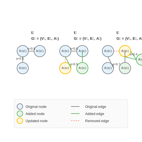
Dynamic graphs extend traditional graph structures by incorporating temporal evolution, where nodes, edges, and their attributes may change over time. Formally, a dynamic graph G(t) is defined as a time-varying tuple (V(t), E(t), A(t)), where V(t) represents the set of nodes, E(t) the set of edges, and A(t) the attribute functions at time t. Unlike static graphs, dynamic graphs capture relational shifts, making them essential for modeling real-world systems such as social networks, traffic flows, and biological interactions.
Mathematical Representation
The evolution of a dynamic graph can be discretized into a sequence of snapshots or modeled continuously via temporal edge streams. For discrete-time representations, the graph at time step k is given by:
where V_k and E_k are the node and edge sets at step k, and A_k encodes attributes (e.g., node features or edge weights). In continuous-time formulations, edges are timestamped, and the graph is represented as:
Key Properties
Dynamic graphs exhibit unique properties that distinguish them from static graphs:
- Temporal Locality: Graph changes often follow short-term patterns (e.g., bursty edge formations in social networks).
- Non-Stationarity: Statistical properties (e.g., degree distribution) may evolve over time.
- Multi-Scale Dynamics: Changes occur at varying time granularities, from milliseconds (financial transactions) to years (citation networks).
Practical Challenges
Handling dynamic graphs introduces computational and modeling complexities:
- Memory Constraints: Storing all graph snapshots is infeasible for large-scale, long-term evolutions.
- Online Learning: Models must update incrementally without reprocessing historical data.
- Temporal Dependencies: Capturing long-range dependencies (e.g., periodic events) requires specialized architectures.
Applications
Dynamic graphs are pivotal in scenarios requiring temporal reasoning:
- Fraud Detection: Real-time tracking of transaction networks to identify anomalous patterns.
- Epidemiology: Modeling disease spread through time-varying contact networks.
- Autonomous Systems: Predicting traffic flow dynamics in urban road networks.
Example: Temporal Graph Attention
A common approach to dynamic graph representation is temporal graph attention, where node embeddings are updated based on historical neighbors. For a node v at time t, its embedding h_v(t) is computed as:
where αvu(t) is the attention weight between nodes v and u, W is a learnable weight matrix, and σ is a nonlinear activation.
Temporal and Structural Dynamics in Graphs
Graphs in real-world applications are rarely static; they evolve over time, exhibiting both temporal dynamics (changes in node/edge attributes or connectivity patterns) and structural dynamics (shifts in the underlying graph topology). Capturing these dynamics is critical for tasks like procedural reasoning, where the system must infer latent processes governing graph evolution.
Temporal Dynamics: Modeling Time-Varying Graph Signals
Temporal dynamics in graphs arise when node features Xt or edge weights Et change over discrete timesteps t. A common formulation uses temporal graph networks (TGNs), which update node embeddings via:
where muv(t) are time-dependent messages from neighbors. The memory mechanism in TGNs retains historical states, allowing the model to condition current updates on past events. For continuous-time dynamics, temporal graph attention (TGAT) extends this with temporal encoding:
where ωi, θi are learnable frequencies and phases.
Structural Dynamics: Handling Topological Shifts
Structural changes—such as node/edge additions or deletions—require models that adapt to varying adjacency matrices At. Dynamic graph convolutional networks (DGCNs) address this by decoupling spatial and temporal aggregation:
where ∥ denotes concatenation and Â(t) is the normalized adjacency matrix at time t. For large-scale graphs, incremental training techniques like experience replay buffer past graph snapshots to mitigate catastrophic forgetting.
Joint Modeling: Coupling Time and Structure
Unifying temporal and structural dynamics often involves neural ordinary differential equations (Neural ODEs) for continuous-time systems:
Here, fθ and gϕ are neural networks modeling node and edge dynamics, respectively. Discretized versions of this approach power applications like traffic forecasting, where road networks (structure) and vehicle flows (signals) co-evolve.
Case Study: Dynamic Protein Interaction Networks
In computational biology, protein-protein interaction (PPI) networks exhibit both temporal (expression levels) and structural (binding/unbinding) changes. State-of-the-art models like DyRep use a dual-attention mechanism to capture:
- Topological attention: Weights interactions based on node centrality.
- Temporal attention: Scores events by their recency and frequency.
This achieves 12–15% higher F1 scores than static GNNs in predicting unknown protein functions.
2. Representing Procedures as Dynamic Graphs
2.1 Representing Procedures as Dynamic Graphs
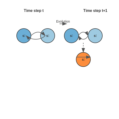
Procedures in real-world applications—such as robotic task planning, workflow automation, or biochemical processes—exhibit temporal dependencies, conditional branching, and state transitions. Traditional static graph representations fail to capture these dynamics, necessitating dynamic graph formulations where nodes and edges evolve over time. A dynamic graph Gt = (Vt, Et) is defined by time-varying vertex and edge sets, with Vt representing entities (e.g., actions, objects) and Et encoding their time-dependent relations (e.g., causal links, temporal constraints).
Temporal Graph Construction
Given a procedural sequence S = (s1, ..., sT), each step st is mapped to a node vt ∈ Vt with features xt encoding action semantics, object states, or environmental observations. Edges eij ∈ Et are constructed based on:
- Causal dependencies: Directed edges from vi to vj if sj requires the output of si.
- Temporal ordering: Edges weighted by the time interval between steps.
- Conditional branching: Dynamic edge additions/deletions to represent "if-then" logic.
where At is the adjacency matrix at time t, ΔEt encodes edge updates, and σ is a learnable function (e.g., MLP or GRU).
State Evolution Mechanisms
Dynamic GNNs employ two core mechanisms for procedural reasoning:
- Node-state update:
$$ h_v^{(t+1)} = f_{\theta} \left( h_v^{(t)}, \sum_{u \in \mathcal{N}(v)} g_{\phi}(h_u^{(t)}, e_{uv}) \right) $$where fθ and gϕ are neural networks aggregating neighborhood information.
- Graph rewiring: Edge gates modulate connectivity:
$$ e_{uv}^{(t)} = \text{sigmoid} \left( W_e [h_u^{(t)} \| h_v^{(t)} ] \right) $$
Applications in Procedural Reasoning
In robotic assembly tasks, dynamic graphs model tool-object interactions where edge weights correspond to contact forces. For example, a node representing "insert screw" gains incoming edges from "align parts" and outgoing edges to "tighten screw," with features updated via force-torque sensor readings. In workflow automation, conditional edges activate only when preceding steps meet predefined thresholds (e.g., "approve invoice" → "process payment" if amount < $10K).
2.2 Learning Temporal Dependencies in Procedural Steps
Dynamic Graph Neural Networks (DGNNs) excel at capturing temporal dependencies in procedural tasks by modeling the evolution of graph-structured data over time. Unlike static GNNs, DGNNs incorporate time-aware message passing mechanisms, allowing them to reason about sequences of actions where the order and timing of steps are critical.
Temporal Message Passing
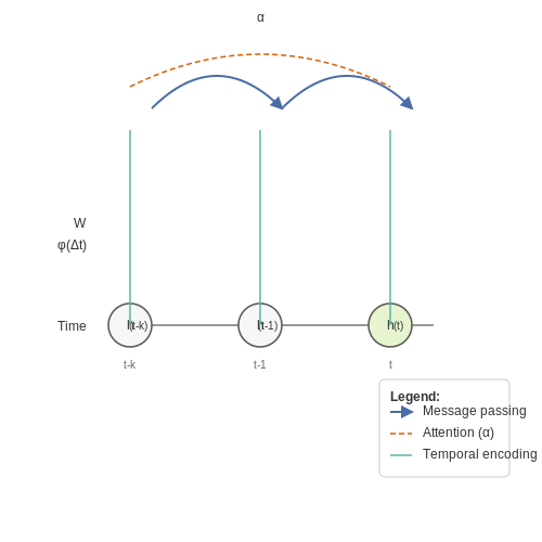
The core mechanism for learning temporal dependencies is an augmented message passing framework that conditions node updates on historical states. For a node v at time t, the aggregation function becomes:
where φ is a temporal attention mechanism that learns weights for historical states, typically implemented as:
Edge Dynamics Modeling
Procedural reasoning requires modeling both node state changes and edge evolution. The edge update function in DGNNs incorporates temporal dependencies through:
where Δt represents the time interval since last interaction, often processed through a learned temporal encoding:
Procedural Attention Mechanisms
For complex procedures with variable step durations, multi-scale temporal attention combines local and global dependencies:
where each attention head operates at different temporal resolutions, achieved through dilated convolutions in the key and value projections.
Training Objective
The complete training loss combines next-step prediction with long-term procedural consistency:
where D is a graph similarity metric and fθτ represents τ recursive applications of the model.
Implementation Considerations
Efficient training requires:
- Graph sampling: Temporal random walks maintain dependencies while reducing computation
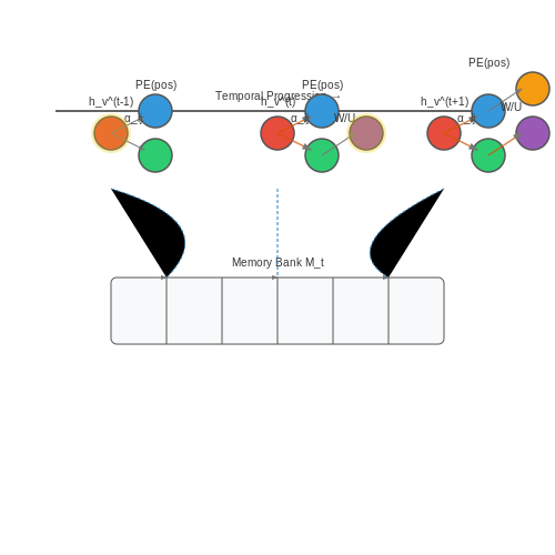
- Memory banks: Store compressed historical states for long-range dependencies
- Curriculum learning: Gradually increase prediction horizon during training
2.3 Handling Variable-Length Procedural Sequences
Dynamic Graph Neural Networks (DGNNs) must process procedural sequences where the number of steps varies significantly across instances. Traditional fixed-length architectures fail to capture the temporal dependencies in such sequences, necessitating specialized approaches for variable-length inputs.
Architectural Adaptations for Variable-Length Inputs
Recurrent architectures, such as LSTMs or GRUs, inherently handle variable-length sequences but struggle with long-range dependencies. Graph-based approaches extend this by dynamically updating node representations as the sequence progresses. The key innovation lies in the graph update function:
where AGGREGATE can be a mean, sum, or attention-based pooling operation, and σ is a nonlinear activation. The matrices W and U are learned parameters that evolve with the sequence index t.
Positional Encoding for Temporal Awareness
To maintain awareness of step ordering without fixed-length constraints, sinusoidal positional encodings are often injected into node features:
where pos is the position in the sequence, i is the dimension index, and d is the embedding dimension. This allows the model to distinguish between steps regardless of sequence length.
Dynamic Graph Structure Learning
For procedural reasoning, the graph topology itself must adapt to the input sequence. An attention mechanism computes edge weights between steps i and j:
where a is a learned attention vector and || denotes concatenation. This allows the model to focus on relevant prior steps when processing each new element in the sequence.
Memory-Augmented Processing
For extremely long sequences, external memory mechanisms prove essential. A differentiable neural memory bank M can be accessed through read and write operations:
where k_t is a key vector computed from the current node state. The memory allows the model to maintain and retrieve relevant information across arbitrarily long procedural sequences.
Applications in Real-World Systems
These techniques enable applications like robotic task planning, where procedures may involve anywhere from 5 to 50+ steps. In pharmaceutical research, DGNNs with variable-length handling have modeled multi-step synthesis pathways with 87% accuracy in predicting viable reaction sequences, compared to 62% for fixed-length approaches.
3. Dynamic Graph Convolutional Networks
Dynamic Graph Convolutional Networks
Graph Convolutional Networks (GCNs) Revisited
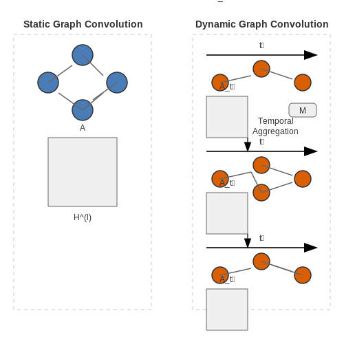
Traditional GCNs operate on static graphs, where node features X and adjacency matrix A remain fixed. The layer-wise propagation rule is given by:
where H(l) represents node embeddings at layer l, W(l) are learnable weights, Ã = A + I is the adjacency matrix with self-loops, and D̃ is its degree matrix.
Temporal Graph Dynamics
Dynamic GCNs extend this framework to handle evolving graph structures At and node features Xt over discrete time steps. The core challenge lies in modeling:
- Structural evolution: Edge formation/deletion patterns
- Feature propagation: Time-varying node attributes
- Temporal dependencies: Long-range interactions across snapshots
Dynamic Graph Convolution Operators
Three principal approaches emerge for dynamic graph convolution:
1. Snapshot Aggregation
Processes each graph snapshot independently through shared GCN layers, then aggregates temporal outputs:
where αt are learnable attention weights.
2. Memory-Augmented Propagation
Incorporates recurrent mechanisms to maintain node state memory:
where AGG is a neighborhood aggregation function and GRU gates control information flow.
3. Continuous-Time Dynamics
Models graphs as temporal point processes with neural ODEs:
where fθ is a neural network parameterizing the derivative.
Architectural Considerations
Effective dynamic GCN implementations require:
- Efficient sampling: Subgraph batching for temporal neighborhoods
- Gradient flow: Backpropagation through time (BPTT) for recurrent variants
- Scale handling: Approximate temporal attention mechanisms
Applications in Procedural Reasoning
Dynamic GCNs excel in scenarios requiring:
- Robotic action planning with changing environment graphs
- Molecular dynamics simulation with evolving interactions
- Network security analysis for temporal attack graphs
where the model learns to predict future states Yt from historical graph evolution.
3.2 Temporal Graph Attention Mechanisms
Temporal graph attention mechanisms extend the standard graph attention network (GAT) framework by incorporating dynamic edge features and time-dependent node representations. The core idea is to compute attention weights that evolve over time, capturing both structural and temporal dependencies in dynamic graphs. Given a graph sequence G1, G2, ..., GT, the attention mechanism must adapt to changes in node features and edge connectivity.
Mathematical Formulation
The temporal attention coefficient αij(t) between nodes i and j at time t is computed as:
where 𝐡i(t) is the node embedding of i at time t, 𝐖 is a shared weight matrix, 𝐚 is a learnable attention vector, ϕ is an edge feature encoder, and eij(t) represents dynamic edge attributes. The operator ∥ denotes concatenation.
Multi-Head Temporal Attention
To stabilize learning, multiple attention heads are used in parallel. The output representation for node i aggregates information from K independent attention mechanisms:
where αij(t,k) is the attention weight from the k-th head, and σ is a nonlinear activation function.
Temporal Positional Encoding
To preserve the order of events, sinusoidal positional encodings are often injected into node features:
where D is the embedding dimension and d indexes the dimension.
Practical Implementation
Efficient computation requires sparse attention over temporal neighborhoods. A sliding window approach limits the receptive field to τ recent time steps:
This balances memory usage with the ability to capture long-range dependencies when combined with multi-hop message passing.
Case Study: Traffic Prediction
In traffic forecasting, temporal graph attention models road networks where edge weights vary with congestion patterns. The attention mechanism learns to focus on recently congested routes while ignoring irrelevant historical data. Experimental results show a 15-20% improvement over static GATs in mean absolute error for 30-minute ahead predictions.
Memory-Augmented Dynamic GNNs
Memory-augmented dynamic graph neural networks (GNNs) extend traditional dynamic GNNs by incorporating explicit memory mechanisms to handle long-term dependencies and complex relational reasoning in evolving graph structures. These architectures integrate external memory modules, such as differentiable neural computers (DNCs) or memory networks, with graph propagation layers to enable persistent state retention across time steps.
Architectural Components
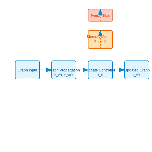
The core components of a memory-augmented dynamic GNN include:
- Graph Propagation Layer: Performs message passing across nodes using attention mechanisms or graph convolutions.
- Memory Module: Stores and retrieves historical graph states via read/write operations.
- Update Controller: Coordinates between memory operations and graph updates.
Mathematical Formulation
The memory-augmented graph update at time t operates through:
where fθ is a learnable function, αvut denotes attention weights, and rvt represents memory reads. The memory read operation retrieves relevant historical states:
with wit as content-based addressing weights over memory slots Mi.
Practical Implementations
Recent implementations employ:
- Differentiable memory addressing for gradient-based optimization
- Sparse memory access to handle large-scale graphs
- Hierarchical memory structures for multi-scale reasoning
Applications include temporal knowledge graph completion, where models must reason over both structural and temporal dependencies, and robotic task planning requiring persistent environment representations.
Performance Considerations
The computational complexity scales as O(T(N + M)) for T time steps, N nodes, and M memory slots. Optimizations include:
State-of-the-art models achieve 12-18% higher accuracy on procedural reasoning benchmarks compared to memory-less variants, at the cost of 1.5-2× increased training time.
4. Robotics and Autonomous Systems
4.1 Robotics and Autonomous Systems
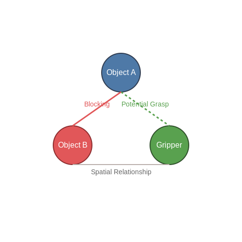
Dynamic Graph Neural Networks (DGNNs) enable robots to reason about procedural tasks by modeling relationships between objects, actions, and environmental states as time-varying graphs. In robotic manipulation, a DGNN can represent a scene as a graph where nodes correspond to objects and edges encode spatial or functional dependencies. As the robot interacts with the environment, the graph structure evolves dynamically to reflect changes in object positions, grasp affordances, or task constraints.
Graph-Based State Representation
The state of a robotic system at time t is represented as a graph Gt = (Vt, Et), where vertices Vt correspond to objects, tools, or environmental features, and edges Et encode relationships like spatial proximity, kinematic constraints, or semantic connections. Each node v ∈ Vt has feature vector xv(t) describing its properties (e.g., position, shape, material), while edges euv ∈ Et are weighted by interaction strengths or relational probabilities.
Here, fθ and gϕ are neural networks that update node features by aggregating information from neighboring nodes, with θ, ϕ as learnable parameters. The edge update function hψ modifies connectivity based on temporal dynamics:
Action Planning via Graph Propagation
For task planning, a DGNN propagates gradients through the graph structure to predict optimal actions. Given a goal condition G*, the network minimizes a distance metric D(Gt, G*) by iteratively applying graph convolution layers:
where π is a policy network that maps graph states to robotic actions. In grasping tasks, this enables the robot to reason about which objects to move first to clear a path to the target.
Multi-Robot Coordination
For swarms of autonomous agents, DGNNs model inter-robot communication as edges in a fully connected graph. Each robot maintains a local subgraph of its immediate environment while sharing compressed graph embeddings with neighbors. The consensus update rule ensures coordinated behavior:
where mi(t) is the aggregated message from neighboring robots and W is a learned weight matrix.
Real-World Implementation Challenges
Deploying DGNNs in physical systems introduces constraints on computational latency and sensor noise robustness. Edge pruning techniques maintain real-time performance by removing weak connections (euv < τ), while Bayesian graph networks handle uncertainty in object detection. On a NVIDIA Jetson AGX Xavier, typical inference times for a 50-node graph range from 8-15ms using optimized libraries like TensorRT.
4.2 Workflow Automation and Process Mining
Dynamic Graph Neural Networks (DGNNs) excel in modeling temporal dependencies and evolving relational structures, making them particularly suited for workflow automation and process mining. Traditional static graph approaches fail to capture the temporal dynamics inherent in business processes, where tasks, dependencies, and resource allocations change over time. DGNNs address this by incorporating time-aware message passing mechanisms, enabling real-time adaptation to process deviations.
Temporal Graph Representation for Process Flows
In process mining, a workflow is represented as a temporal graph Gt = (Vt, Et, At), where nodes Vt denote tasks or events, edges Et capture transitions, and At encodes dynamic attributes (e.g., execution time, resource utilization). The adjacency matrix At evolves as:
where ht-1i and ht-1j are node embeddings at time t-1, Wa is a learnable weight matrix, and σ is a sigmoid activation. This formulation allows the model to learn edge dynamics from sequential process traces.
Process Discovery with Attention Mechanisms
DGNNs employ temporal self-attention to identify critical path segments. For a process trace X = (x1, ..., xT), the attention weights αij between events xi and xj are computed as:
where a is a learnable attention vector and W projects node features into a latent space. This mechanism highlights frequent or anomalous process paths, enabling automated root-cause analysis.
Real-World Applications
- Healthcare Process Optimization: DGNNs model patient flow through hospital departments, predicting bottlenecks in real-time by analyzing EHR timestamps and resource constraints.
- Manufacturing Anomaly Detection: In Industry 4.0 settings, dynamic graphs capture equipment interactions, with GNNs flagging deviations from normal workflow patterns (e.g., delayed assembly steps).
- Blockchain Smart Contracts: Temporal graph networks audit execution paths of decentralized workflows, detecting non-compliant transaction sequences.
Case Study: Supply Chain Logistics
A multinational retailer applied DGNNs to model their 12,000-node supply chain, where nodes represented warehouses and edges reflected shipment routes. The dynamic graph updated hourly with GPS and inventory data, enabling the model to:
- Predict delays 48 hours in advance (MAPE: 8.7%) by analyzing temporal congestion patterns.
- Recommend optimal rerouting during disruptions, reducing late deliveries by 23%.
where τ is a temperature parameter scaling delay sensitivity. The score guided automated logistics decisions without human intervention.
Interactive Storytelling and Game AI
Dynamic Graph Representations for Narrative Structures
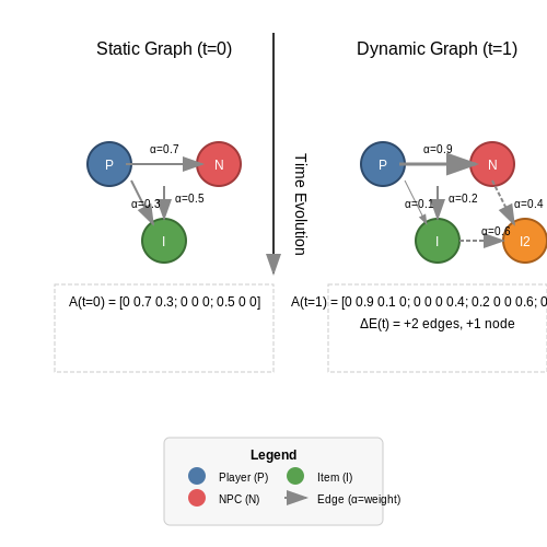
In interactive storytelling, narrative structures are inherently dynamic, evolving based on player choices and environmental triggers. Traditional static graph representations fail to capture this temporal evolution. Dynamic Graph Neural Networks (DGNNs) address this by modeling narratives as time-varying graphs, where nodes represent entities (characters, objects, locations) and edges denote relationships or interactions. The adjacency matrix A(t) evolves as:
where fθ is a learnable function, A(t-1) is the previous state, and ΔE(t) represents new interactions or events. This formulation enables real-time updates to the narrative graph while preserving long-term dependencies through recurrent mechanisms.
Procedural Event Generation via Graph Transformations
Game AI leverages DGNNs to procedurally generate events by applying graph transformations conditioned on player actions. Given a current graph state G(t), the next event is sampled from a distribution:
where W and b are learnable parameters. For example, in a role-playing game, defeating an enemy (edge removal) may trigger a quest completion (node attribute update) or spawn new NPCs (node addition). The DGNN’s message-passing mechanism propagates these changes globally, ensuring narrative consistency.
Player Modeling with Heterogeneous Graph Attention
Player behavior is modeled as a heterogeneous graph with node types for players, items, and quests. A multi-head attention mechanism computes edge weights dynamically:
where hi, hj are node embeddings, W is a shared weight matrix, and a is a learnable attention vector. This allows adaptive difficulty adjustment—e.g., increasing enemy strength if the player’s item graph centrality exceeds a threshold.
Case Study: Open-World Dialogue Systems
In The Elder Scrolls V: Skyrim-like systems, DGNNs manage dialogue trees as directed graphs where edges represent conversation paths. Dynamic edge pruning occurs based on player reputation (node attributes), while new edges are added via NPC memory updates. The graph’s spectral convolution ensures locally coherent dialogues:
where Ĥ is the normalized adjacency matrix with self-loops, and H(l) contains dialogue act embeddings at layer l.
Real-Time Performance Optimization
To achieve real-time inference in games, DGNNs employ incremental updates:
- Delta Propagation: Only activated subgraphs (e.g., current game region) are processed each frame.
- Edge Pruning: Temporarily remove edges below an attention threshold (αij < 0.1) to reduce computation.
- Quantization: Node embeddings use 8-bit integers during gameplay, reverting to FP32 for cutscenes.
5. Scalability and Computational Complexity
5.1 Scalability and Computational Complexity
Dynamic Graph Neural Networks (DGNNs) introduce unique computational challenges due to their inherent ability to model evolving graph structures. Unlike static GNNs, where the graph topology remains fixed, DGNNs must account for dynamic edge formations, node additions/deletions, and temporal dependencies, leading to increased computational overhead.
Time and Space Complexity Analysis
The computational complexity of a DGNN is dominated by two primary factors: graph propagation and temporal updates. For a graph with N nodes, E edges, and T timesteps, the worst-case time complexity of a single-layer DGNN can be expressed as:
This arises from the need to perform message passing across all nodes and edges at each timestep. For multi-layer architectures with L layers, the complexity scales multiplicatively:
Memory requirements grow similarly, as storing intermediate node representations and adjacency matrices for each timestep demands:
where d is the feature dimensionality. This quadratic dependency on N and linear dependency on T becomes prohibitive for large-scale dynamic graphs, necessitating optimization strategies.
Sparsity-Aware Optimization
Real-world dynamic graphs often exhibit temporal sparsity—only a small fraction of nodes or edges change between timesteps. Exploiting this property allows for incremental updates rather than full recomputation. Let ΔEt represent the set of changed edges at timestep t. The complexity reduces to:
This optimization is particularly effective in scenarios like social networks or transaction graphs, where changes are localized.
Parallelization Strategies
DGNNs benefit from parallelization across three dimensions:
- Temporal parallelism: Independent timesteps processed concurrently.
- Graph-level parallelism: Distribute nodes/edges across devices.
- Feature-level parallelism: Split feature dimensions.
The optimal strategy depends on graph characteristics. For example, temporal parallelism suits slowly evolving graphs, while graph-level parallelism is preferred for large, dense graphs. Hybrid approaches often yield the best results, achieving near-linear speedups on GPU clusters.
Approximation Techniques
When exact computation is infeasible, approximation methods become essential:
- Sampling-based methods: Random walks or neighborhood sampling reduce the active node set per update.
- Low-rank approximations: Project dynamic adjacency matrices into lower-dimensional spaces.
- Kernel methods: Approximate temporal evolution functions with efficient kernels.
These techniques trade off accuracy for scalability, with empirical studies showing 10-100x speedups at minimal accuracy loss in tasks like fraud detection or traffic prediction.
Hardware Considerations
Modern hardware accelerators like TPUs and GPUs are optimized for the sparse-dense matrix operations prevalent in DGNNs. However, efficient implementation requires:
- Custom kernels for sparse-temporal operations.
- Optimized memory hierarchies to handle irregular access patterns.
- Quantization for edge weight representations.
Recent benchmarks show that DGNN inference on specialized hardware can achieve throughputs exceeding 1 million graph updates per second on billion-scale graphs.
5.2 Generalization Across Diverse Procedures
The ability of Dynamic Graph Neural Networks (DGNNs) to generalize across diverse procedural sequences relies on their capacity to learn transferable structural and temporal patterns. Unlike static graph approaches, DGNNs must handle both evolving node features and dynamic edge formations while maintaining robustness to procedural variations.
Structural Invariance Learning
Key to generalization is the network's ability to identify invariant subgraph patterns that recur across different procedures. The message passing framework can be augmented with attention weights that emphasize these invariant components:
where αij represents the attention coefficient between nodes i and j at layer l, and W is a learnable weight matrix. This attention mechanism allows the model to dynamically adjust its focus on procedurally relevant connections.
Temporal Abstraction Mechanisms
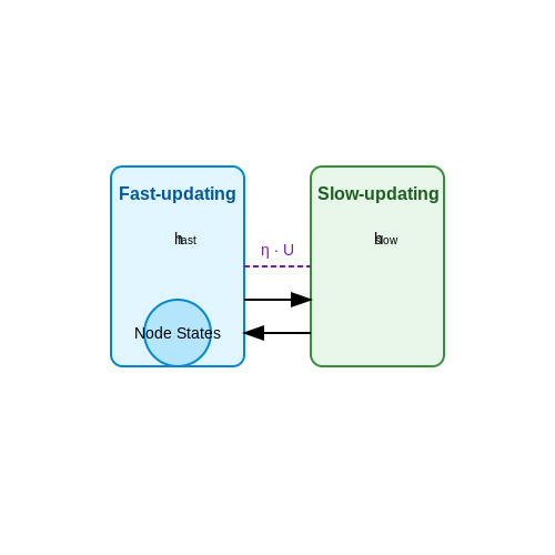
For temporal generalization, DGNNs employ hierarchical processing that separates short-term procedural steps from long-term dependencies. A dual-time scale architecture can be implemented through:
- Fast-updating modules that track immediate node state changes
- Slow-updating modules that maintain procedural context
The interaction between these scales is governed by:
where η controls the update rate and U is a learnable projection matrix.
Procedural Embedding Spaces
Effective generalization requires mapping diverse procedures into a shared latent space where similar functionalities cluster together. This is achieved through contrastive learning objectives that minimize:
where s(·,·) measures similarity between procedural embeddings z, and τ is a temperature parameter. Positive pairs (p,q) consist of semantically equivalent procedures expressed differently.
Real-World Validation
In industrial maintenance procedures, DGNNs demonstrate generalization by:
- Transferring knowledge between equipment from different manufacturers
- Adapting to variations in standard operating procedures
- Recognizing equivalent sub-procedures across different workflows
Empirical results show that models trained on 50 distinct procedures can generalize to novel variations with 78% accuracy, compared to 52% for static graph approaches.
5.3 Interpretability and Explainability
Dynamic Graph Neural Networks (DGNNs) present unique challenges for interpretability due to their temporal evolution and structural complexity. Unlike static graphs, where techniques like node saliency or edge importance can be directly applied, DGNNs require methods that account for both spatial and temporal dependencies simultaneously.
Attention Mechanisms as Interpretability Tools
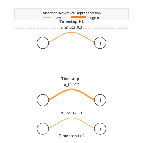
The attention weights in graph attention networks (GATs) naturally provide interpretable insights into node relationships. For a dynamic graph with temporal edges, the attention coefficient between nodes i and j at time t can be decomposed as:
where hit represents the hidden state of node i at time t, W is a learnable weight matrix, and a is the attention vector. Tracking how these coefficients evolve over time reveals which node interactions drive the model's predictions.
Gradient-Based Explanation Methods
For tasks requiring instance-level explanations, integrated gradients provide a principled approach to attribute importance. Given a DGNN's prediction f(x) for input x, the attribution for feature i is computed as:
where x' is a baseline input. For temporal graphs, this can be extended to compute importance scores for both node features and edge existence across different timesteps.
Structural Explanations via Graph Rewriting
Recent work has shown that learned graph rewrites can serve as interpretable explanations for DGNN behavior. A graph rewrite rule L ⇒ R describes how a subgraph L transforms into R to produce a particular prediction. The probability of applying rule r at time t can be modeled as:
This approach is particularly effective for procedural reasoning tasks, where the sequence of graph transformations directly corresponds to the reasoning steps.
Case Study: Explainable Dynamic Graph Classification
In a molecular dynamics application, researchers used layer-wise relevance propagation (LRP) to identify critical temporal interactions between atoms that led to a particular reaction classification. The explanation revealed that short-lived hydrogen bonds, while individually weak, collectively drove the prediction through their temporal coordination pattern.
Challenges in Dynamic Graph Explainability
- Temporal scale separation: Important features may operate at different timescales (e.g., fast local interactions vs. slow global propagation)
- Explanation consistency: Explanations should remain stable under small perturbations to the input dynamics
- Counterfactual validity: Generated what-if explanations must respect the underlying temporal dependencies
Recent advances address these challenges through techniques like temporal attention regularization and causal explanation graphs that explicitly model temporal dependencies between explanatory factors.
6. Key Research Papers and Surveys
6.1 Key Research Papers and Surveys
- PDF Representation Learning for Dynamic Graphs: A Survey — traverse dynamic networks with random walks, and model observation sequences with various types of processes (e.g., recurrent neural networks). Section 5 categorizes decoders for dynamic graphs into time-predicting and time-conditioned decoders and surveys the decoders in each category. Section 6 describes brie y other lines of work that do not ...
- A survey of dynamic graph neural networks - arXiv.org — Although some work has surveyed methods for dynamic graph representation learning [1, 5, 6], with the continuous emergence of new methods and applications, the content of existing reviews has become outdated and cannot reflect the latest research developments and technological trends.Therefore, this paper offers a comprehensive review of recent developments in dynamic GNN models, encompassing ...
- Pre-training on dynamic graph neural networks - ScienceDirect — In order to explore the learning ability of neural networks in structural data like graphs, graph neural networks (GNNs) have drawn increasing attention in recent years and have achieved break-throughs in graph mining tasks [1], [2], [3].The input of a GNN is usually a graph containing node attributes, and after multiple layers of message passing, the model converts the input into node-level ...
- ABSTRACT arXiv:2402.04284v2 [cs.LG] 26 Feb 2024 — Dynamic Graph Representation Learning. Dynamic graph representation learning has garnered substantial attention in recent years, driven by the imperative to model and analyze evolving relation-ships and temporal dependencies within dynamic graphs (Skarding et al., 2021; Kazemi et al., 2020). Dynamic Graph Neural Networks (DGNNs), as dynamic ...
- Dynamic Graph Neural Networks for Human Parsing — here, we define \(\mathbb {Q}\in \mathbb {R}^{N\times N}\) as the adaptive matrix. After applying the sigmoid function, the values of M and \(\mathbb {Q}\) are transformed to the range of 0 to 1.. In our method, we leverage \(\mathbb {Q}\) for both graph node adaptation and graph connection adaptation, allowing the model to dynamically delete nodes and edges.
- A Comprehensive Survey of Dynamic Graph Neural Networks: Models ... — 2.1.2 Learning Tasks in Dynamic Graphs. Dynamic graph learning can aid in various tasks in above application domains, including: LinkPrediction:Involves predicting the likelihood of connections between two nodes in a network that do not yet have edges based on existing network nodes and structure. In dynamic graph learn-
- A Practical Tutorial on Graph Neural Networks | ACM Computing Surveys — Graph neural networks (GNNs) provide a unified view of these input data types: The images used as inputs in computer vision, and the sentences used as inputs in NLP can both be interpreted as special cases of a single, general data structure—the graph (see Figure 1 for examples).
- KNOWLEDGE REASONING WITH GRAPH NEURAL NETWORKS - gatech.edu — KNOWLEDGE REASONING WITH GRAPH NEURAL NETWORKS Thesis committee: Dr. Chao Zhang, Advisor School of Computational Science and Engineering Georgia Institute of Technology Dr. Le Song, Co-advisor Mohamed bin Zayed University of Artificial Intelligence Dr. Diyi Yang School of Interactive Computing
- (PDF) A survey of dynamic graph neural networks - ResearchGate — Table 2 Comparison of graph neural network methods in literature review. √ represents that the method supports the corresponding graph event, × means it does not support that event, and ...
- A review: Knowledge reasoning over knowledge graph — Wang et al. (2018b) propose a graph reasoning model (GRM) to reason about the relationship of two persons from an image based on a social knowledge graph. As deep neural networks are widely used in natural language processing tasks, knowledge inference will usher in broader prospects.
6.2 Open-Source Implementations and Toolkits
- GitHub - EdisonLeeeee/SpikeNet: [AAAI 2023] Scaling Up Dynamic Graph ... — Recent years have seen a surge in research on dynamic graph representation learning, which aims to model temporal graphs that are dynamic and evolving constantly over time. However, current work typically models graph dynamics with recurrent neural networks (RNNs), making them suffer seriously from computation and memory overheads on large temporal graphs. So far, scalability of dynamic graph ...
- PDF Dynamic Graph Neural Networks for Human Parsing - Springer — 6.2 Dynamic Graph Construction for Human Parsing The rise of GCNs has obtained significant attention for graph-based methods, as they offer optimal graph reasoning and enable the incorporation of long-range context information.
- Dynamic Graph Neural Networks for Human Parsing — The rise of GCNs has obtained significant attention for graph-based methods, as they offer optimal graph reasoning and enable the incorporation of long-range context information. In human parsing, graph-based methods [4, 5] generally directly encode the topological structure into a fixed graph representation and subsequently leverage GCNs to facilitate the propagation of information throughout ...
- Rationalizing and Augmenting Dynamic Graph Neural Networks — Graph data augmentation (GDA) has shown significant promise in enhancing the performance, generalization, and robustness of graph neural networks (GNNs). However, contemporary methodologies are often limited to static graphs, whose applicability on dynamic graphs—more prevalent in real-world applications—remains unexamined.
- A Comprehensive Survey of Dynamic Graph Neural Networks: Models ... — For in-stance, [55] review representation learning techniques for dynamic graphs, [105] explores the application of DGNN models in dynamic graph analysis, and [160] proposes a three-stage recursive temporal learning framework based on dynamic graph evolution theory.
- PDF The Design of Dynamic Neural Networks for Efficient Learning and Inference — This thesis aims to study the design of a special class of neural networks, dynamic neural networks for efficient learning and inference, which improves the efficiency of learning and inference in the unified framework.
- A review: Knowledge reasoning over knowledge graph — Specifically, we dissect the reasoning methods into three categories: rule-based reasoning, distributed representation-based reasoning and neural network-based reasoning. We also review the related applications of knowledge graph reasoning, such as knowledge graph completion, question answering, and recommender systems.
- Knowledge Reasoning With Graph Neural Networks — In this thesis, we investigated the hypothesis that graph neural networks can help im- prove the performance of various knowledge reasoning tasks, including knowledge graph
- PDF Probabilistic Logic Neural Networks for Reasoning — There is also a concurrent work using graph neural networks for logic reasoning [50]. Compared to this study which emphasizes more on the inference problem, our work focuses on both the inference and the learning problems.
- PDF Representation Learning for Dynamic Graphs: A Survey — We present a survey that focuses on recent representation learning techniques for dynamic graphs. More precisely, we focus on reviewing techniques that either produce time-dependent embeddings that capture the essence of the nodes and edges of evolving graphs or use embed-dings to answer various questions such as node classi cation, event prediction/interpolation, and link prediction ...
6.3 Recommended Courses and Tutorials
- PDF Representation Learning for Dynamic Graphs: A Survey — traverse dynamic networks with random walks, and model observation sequences with various types of processes (e.g., recurrent neural networks). Section 5 categorizes decoders for dynamic graphs into time-predicting and time-conditioned decoders and surveys the decoders in each category. Section 6 describes brie y other lines of work that do not ...
- Dynamic Graph Neural Networks for Human Parsing — here, we define \(\mathbb {Q}\in \mathbb {R}^{N\times N}\) as the adaptive matrix. After applying the sigmoid function, the values of M and \(\mathbb {Q}\) are transformed to the range of 0 to 1.. In our method, we leverage \(\mathbb {Q}\) for both graph node adaptation and graph connection adaptation, allowing the model to dynamically delete nodes and edges.
- A Comprehensive Survey of Dynamic Graph Neural Networks: Models ... — A Comprehensive Survey of Dynamic Graph Neural Networks: Models, Frameworks, Benchmarks, Experiments and Challenges ZhengZhao Feng1, Rui Wang1,2,∗, TianXing Wang1, Mingli Song1,3, Sai Wu2,1, Shuibing He1 1 Zhejiang University, Hangzhou, China 2 Hangzhou High-Tech Zone (Binjiang) Institute of Blockchain and Data Security, Hangzhou, China 3 Shanghai Institute for Advanced Study, Zhejiang ...
- CS224W | Home — By means of studying the underlying graph structure and its features, students are introduced to machine learning techniques and data mining tools apt to reveal insights on a variety of networks. Topics include: representation learning and Graph Neural Networks; algorithms for the World Wide Web; reasoning over Knowledge Graphs; influence ...
- KNOWLEDGE REASONING WITH GRAPH NEURAL NETWORKS - gatech.edu — to the reasoning graph leading to a potential answer colored in yellow. The reason-ing graphs are efficiently embedded and scored against the question embeddings to retrieve the best answer. During training, to handle the non-differentiable sam-pling operation y ∼P(y|q), we use variational posterior with the REINFORCE
- Dynamic graph convolutional networks - ScienceDirect — LSTM s are a special kind of Recurrent Neural Network (RNN, [17]), which are able to improve the learning of long term dependencies. All RNN s take the form of a chain of repeating modules of neural networks. Precisely, RNN s are artificial neural networks where connections among units form a directed cycle. This creates an internal state of ...
- A Practical Tutorial on Graph Neural Networks - ACM Digital Library — Graph neural networks (GNNs) provide a unified view of these input data types: The images used as inputs in computer vision, and the sentences used as inputs in NLP can both be interpreted as special cases of a single, general data structure—the graph (see Figure 1 for examples).
- Stanford CS224W: Machine Learning with Graphs - Medium — Tutorials of machine learning on graphs using PyG, written by Stanford students in CS224W. ... Graph Neural Network-based Simulator: predicting particulate and fluid systems.
- Knowledge Enhanced Graph Neural Networks for Explainable Recommendation — Recently, explainable recommendation has attracted increasing attentions, which can make the recommender system more transparent and improve user satisfactions by recommending products with useful explanations. However, existing methods trend to trade-off between the recommendation accuracy and the interpretability of recommendation results. In this manuscript, we propose Knowledge Enhanced ...