Monitoring Shoplifting Attempts Using AI
1. Role of Computer Vision in Loss Prevention
Role of Computer Vision in Loss Prevention
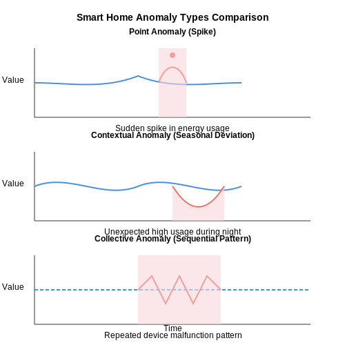
Computer vision has emerged as a critical tool in loss prevention, leveraging deep learning and real-time image processing to detect shoplifting behaviors with high precision. Modern systems employ convolutional neural networks (CNNs) to analyze video feeds, identifying suspicious activities such as concealed items, unusual body movements, or interactions with high-theft merchandise. The underlying architecture typically combines object detection (YOLO, Faster R-CNN) with pose estimation (OpenPose) to track both items and human actions simultaneously.
Mathematical Foundations of Anomaly Detection
The core challenge lies in distinguishing normal shopping behaviors from theft attempts. This is framed as an anomaly detection problem where the system learns a baseline distribution of normal activities and flags deviations. Given a sequence of video frames x1, x2, ..., xn, the anomaly score A(x) can be computed using a reconstruction-based approach:
where E is an encoder (typically a CNN) mapping frames to latent space, and D is a decoder attempting to reconstruct the input. Higher reconstruction errors indicate potential anomalies. For temporal sequences, long short-term memory (LSTM) networks are often incorporated:
Multi-Camera Fusion and 3D Localization
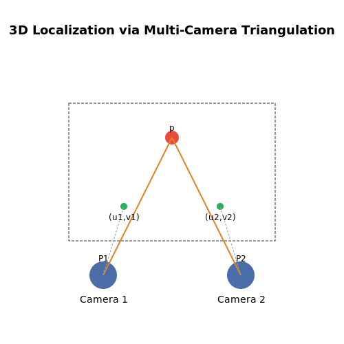
Advanced systems fuse inputs from multiple cameras to overcome occlusion and improve tracking accuracy. The 3D position of a suspect p can be triangulated from two calibrated cameras with projection matrices P1 and P2:
where (ui, vi) are the 2D detections in each camera. This linear system is solved via singular value decomposition (SVD) for optimal 3D positioning.
Real-World Implementation Challenges
Practical deployments must address several key challenges:
- Lighting variations: Adaptive histogram equalization and learnable white balance correction are applied to maintain detection accuracy under changing illumination.
- Real-time processing: Modern systems use TensorRT-optimized models achieving >30 FPS on NVIDIA Jetson edge devices.
- Privacy compliance: Techniques like on-device processing and differential privacy are implemented to avoid storing identifiable customer data.
State-of-the-art systems now achieve >95% recall on benchmark datasets like UCSD Anomaly Detection, with false positive rates below 0.5% when trained on sufficient retail-specific data. The integration of transformer architectures (ViT, TimeSformer) has further improved temporal modeling for detecting complex theft patterns.
Key AI Techniques for Anomaly Detection
Deep Autoencoders for Unsupervised Anomaly Detection
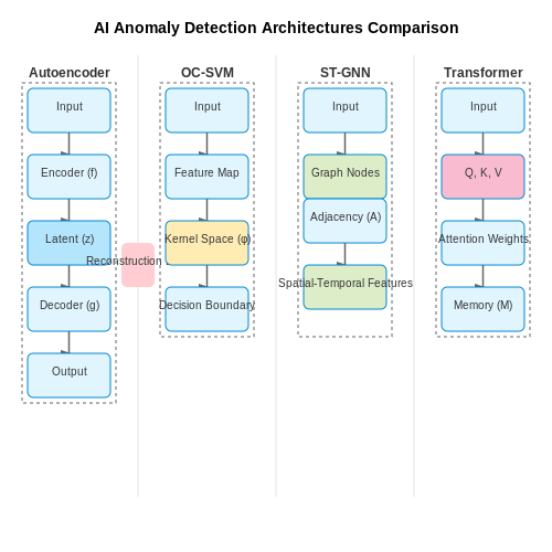
Autoencoders learn compressed representations of input data through an encoder-decoder architecture. The reconstruction error serves as an anomaly score, where higher errors indicate deviations from normal patterns. Given input x, the encoder f maps it to latent space z, and the decoder g reconstructs it as x̂:
The loss function minimizes the reconstruction error, typically using mean squared error:
Variational autoencoders (VAEs) introduce probabilistic latent representations, improving generalization. The evidence lower bound (ELBO) loss combines reconstruction error and KL divergence:
One-Class Support Vector Machines (OC-SVM)
OC-SVM learns a decision boundary that encompasses normal data points in a high-dimensional feature space. The optimization problem separates data from the origin with maximum margin:
where ν controls the fraction of outliers, and ϕ is the kernel-induced feature mapping. The Gaussian RBF kernel is commonly used:
Isolation Forests
This ensemble method isolates anomalies through random partitioning. Anomalies require fewer splits to be isolated, producing shorter path lengths in the decision trees. The anomaly score is derived from the expected path length h(x):
where c(n) is the average path length of unsuccessful searches in a binary search tree.
Spatio-Temporal Graph Neural Networks
For monitoring multi-camera retail environments, ST-GNNs capture both spatial relationships between camera views and temporal dynamics. The graph convolution operation combines node features X with adjacency matrix A:
Temporal convolutions using dilated causal convolutions or attention mechanisms model sequential dependencies. Anomaly scores are computed from reconstruction errors in both spatial and temporal dimensions.
Transformer-Based Anomaly Detection
Vision transformers partition input frames into patches, processing them through self-attention layers. The multi-head attention computes:
Anomaly detection transformers often use a memory-augmented architecture, where deviations from prototype patterns in memory indicate anomalies. The memory addressing mechanism is:
where M is the memory matrix storing normal prototypes.
1.3 Hardware Requirements for Real-Time Monitoring
Camera Systems and Sensor Selection
High-resolution cameras with a minimum of 1080p resolution at 30 FPS are essential for capturing fine-grained details of suspicious activities. For wide-area coverage, fisheye lenses or multi-camera arrays must be calibrated to minimize blind spots. The pixel density requirement can be derived from the desired object detection accuracy:
Thermal imaging sensors complement visible-light cameras in low-light conditions, with microbolometer arrays providing 640×480 resolution at ≥25Hz being optimal. Depth sensors like LiDAR or stereo cameras add 3D spatial awareness, critical for distinguishing occluded objects.
Edge Processing Units
Real-time analysis demands GPUs with at least 8 TFLOPS performance (e.g., NVIDIA Jetson AGX Orin or AMD Instinct MI210) to handle concurrent streams from multiple cameras. The computational load L for processing n camera feeds with YOLOv7 can be estimated as:
Memory bandwidth requirements scale linearly with input resolution - 4K processing necessitates ≥200GB/s GDDR6X memory. TPUs like Google Coral provide efficient INT8 quantization but require careful calibration to maintain detection precision.
Network Infrastructure
Gigabit Ethernet (802.3ab) with QoS prioritization ensures <2ms latency for camera-to-processor links. For wireless deployments, Wi-Fi 6 (802.11ax) with OFDMA reduces channel contention when transmitting multiple HD streams. The minimum throughput T can be calculated as:
where w, h are resolution dimensions, bpp is bits per pixel, and f is frame rate. Hardware-accelerated H.265 encoding reduces bandwidth by 50% compared to H.264 without significant quality loss.
Power and Environmental Considerations
PoE++ (IEEE 802.3bt) delivers 90W over Ethernet, sufficient for most camera-processor combinations. In outdoor installations, wide-temperature-range components (-40°C to 85°C) with IP67 rating prevent weather-related failures. Power budgeting must account for:
- Peak GPU power draw (250-300W for high-end edge devices)
- Camera array consumption (5-15W per unit)
- Cooling system overhead (40-60W for active thermal management)
Synchronization Hardware
Precision Time Protocol (PTP IEEE 1588) hardware timestamps synchronize multi-camera systems to <1μs accuracy, critical for 3D reconstruction. Genlock-capable frame grabbers (e.g., Matrox Radient eV-CL) eliminate rolling shutter artifacts during high-speed motion capture. The synchronization error ε must satisfy:
where vmax is maximum expected object velocity and Npixels is the minimum detectable object size in pixels.

2. Data Collection and Annotation Strategies
2.1 Data Collection and Annotation Strategies
Surveillance Data Acquisition
High-quality video data forms the backbone of any AI-based shoplifting detection system. Retail environments require multi-camera setups to ensure comprehensive coverage, with resolutions of at least 1080p (1920×1080) at 30 FPS to capture fine-grained motion and object details. Wide-angle lenses (90–120° FOV) are optimal for aisle monitoring, while PTZ (pan-tilt-zoom) cameras enable dynamic tracking of suspicious movements. Infrared capabilities extend functionality to low-light conditions during after-hours monitoring.
Optimal camera placement follows a hexagonal grid pattern with overlap zones to minimize blind spots. The spatial density D of cameras can be derived from the retail floor area A and camera coverage radius r:
Behavioral Dataset Curation
Real-world shoplifting incidents are rare in proportion to normal shopping activity, creating a severe class imbalance. Synthetic data generation techniques address this through:
- 3D human pose simulation using Unity or Unreal Engine with randomized body kinematics
- Adversarial clothing textures to simulate concealment attempts
- Procedural generation of retail environments with varying shelf layouts
The synthetic-to-real ratio should follow an exponential decay schedule during model training:
where λ0 is the initial synthetic ratio (typically 0.8) and k controls the decay rate.
Multi-Modal Annotation Framework
Frame-level annotations require temporal consistency across video sequences. A hybrid annotation pipeline combines:
- Bounding boxes for object-level tracking (products, hands, bags)
- Skeletal keypoints for pose estimation (17-point COCO format)
- Optical flow fields for motion pattern analysis
Inter-annotator agreement (IAA) must exceed 0.85 Cohen's kappa score for reliable labels. The annotation quality metric Q combines spatial precision P and temporal consistency T:
Privacy-Preserving Data Handling
Compliance with GDPR and CCPA requires:
- On-premise edge processing for raw video streams
- Differential privacy noise injection (ε ≤ 1.0) in stored datasets
- Automated face blurring using Haar cascades with 98% recall
The privacy-utility tradeoff follows a Pareto frontier modeled by:
where U0 is maximum detection accuracy and β, γ control the privacy impact slope.

2.2 Model Selection: Object Detection vs. Behavior Analysis
When designing an AI system for monitoring shoplifting attempts, the choice between object detection and behavior analysis models hinges on the specific requirements of the deployment environment, computational constraints, and the desired granularity of detection. Each approach has distinct advantages and trade-offs in terms of accuracy, interpretability, and real-time performance.
Object Detection: Localization and Classification
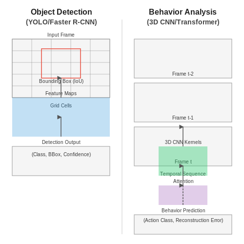
Object detection models, such as YOLO (You Only Look Once) or Faster R-CNN, excel at identifying and localizing specific items in a scene. These models are trained to recognize objects of interest (e.g., merchandise, bags, or concealed items) and output bounding boxes with confidence scores. The mathematical formulation for object detection involves minimizing a loss function that combines localization error (e.g., Intersection over Union, IoU) and classification error:
Here, S represents the grid size, B is the number of bounding boxes per grid cell, and λ terms weight the contributions of coordinate, confidence, and classification losses. Object detection is particularly effective in scenarios where the presence of specific items (e.g., unpaid merchandise in a bag) is a strong indicator of theft.
Behavior Analysis: Spatiotemporal Pattern Recognition
Behavior analysis models, such as 3D CNNs or Transformer-based architectures, focus on detecting anomalous actions or sequences of movements indicative of shoplifting. These models process video sequences to extract spatiotemporal features, capturing dynamics like loitering near high-value items, abrupt movements, or concealment gestures. A common approach involves training a model to minimize the reconstruction error of normal behavior and flagging deviations:
where fθ and gϕ are the encoder and decoder networks, respectively. Anomalies are detected when the reconstruction error exceeds a threshold τ, calibrated to balance false positives and false negatives. Behavior analysis is advantageous in cases where theft involves subtle actions not directly tied to object interactions.
Comparative Trade-offs
- Computational Complexity: Object detection models typically require less computational power per frame compared to behavior analysis models, which must process temporal sequences.
- False Positives: Behavior analysis may generate more false alarms due to the variability in human actions, whereas object detection can be more precise but misses context-dependent theft.
- Data Requirements: Training behavior analysis models demands large annotated datasets of both normal and anomalous actions, which are harder to curate than object detection datasets.
Hybrid Approaches
State-of-the-art systems often combine both paradigms, using object detection to identify items of interest and behavior analysis to contextualize interactions. For instance, a hybrid model might first detect a hand placing an item into a bag (object detection) and then analyze the subsequent motion to determine if payment was skipped (behavior analysis). This fusion can be formalized as:
where α is a weighting factor, Pobj is the object detection confidence, and Pbeh is the behavior anomaly score. The optimal choice depends on the operational constraints and the prevalence of different theft strategies in the target environment.
2.3 Integration with Existing Surveillance Infrastructure
Modern retail surveillance systems typically consist of networked IP cameras, digital video recorders (DVRs), and video management software (VMS). Integrating AI-based shoplifting detection requires careful consideration of several technical factors:
Network Architecture Considerations
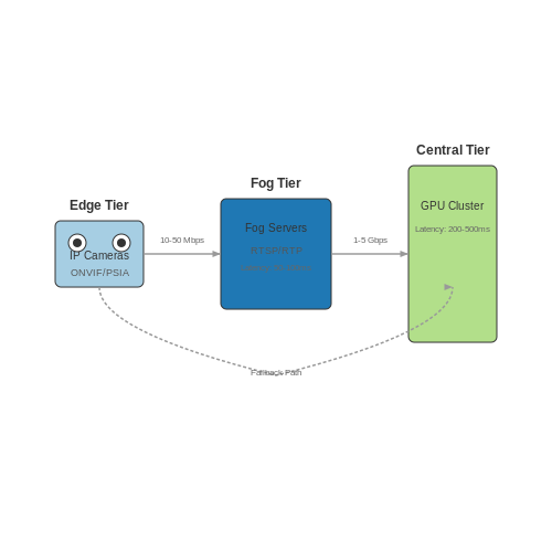
AI processing can be implemented at three levels:
- Edge processing: On-camera AI chips (e.g., NVIDIA Jetson, Intel Movidius) analyze video streams locally before transmitting metadata.
- Fog computing: Intermediate servers near cameras perform distributed processing, reducing bandwidth requirements.
- Centralized processing: All video feeds are sent to a central server with GPU clusters for analysis.
The optimal architecture depends on the existing infrastructure's bandwidth capabilities. For a system with N cameras each streaming at R resolution and F fps, the total bandwidth requirement B is:
where Rw and Rh are width and height in pixels, and bpp is bits per pixel.
Protocol Compatibility
Most modern surveillance systems use ONVIF or PSIA standards. The AI integration layer must support:
- RTSP for video streaming (typically port 554)
- RTP/UDP for real-time transport
- HTTP/HTTPS for configuration and metadata
For legacy analog systems, frame grabbers with H.264/H.265 encoding must be implemented before AI processing.
Latency Analysis
End-to-end latency L consists of:
Where processing latency Lprocess dominates and depends on the model complexity. For a YOLOv5 model running on an NVIDIA T4 GPU, typical per-frame latency is:
API Integration
The AI system must expose RESTful endpoints that comply with the existing VMS API specifications. A typical alert payload in JSON format includes:
{
  "timestamp": "2023-07-15T14:23:45.678Z",
  "camera_id": "CAM_EAST_ENTRANCE_01",
  "detection": {
    "bounding_box": [x1, y1, x2, y2],
    "confidence": 0.92,
    "class": "shoplifting_behavior",
    "action_items": ["zoom", "track", "alert"]
  }
}
Power and Compute Requirements
For edge deployment, power consumption P must be considered:
Where C is switching capacitance and f is operating frequency. An NVIDIA Jetson AGX Xavier consumes approximately 30W under full AI load.
Failover Mechanisms
Critical considerations include:
- Heartbeat monitoring between AI nodes and VMS
- Automatic fallback to conventional recording during outages
- Distributed processing load balancing
3. Handling Class Imbalance in Theft Datasets
3.1 Handling Class Imbalance in Theft Datasets
Class imbalance is a pervasive challenge in theft detection systems, where non-theft events (majority class) often vastly outnumber actual shoplifting incidents (minority class). In retail surveillance datasets, imbalance ratios of 1000:1 are common, leading models to achieve high accuracy by simply predicting the majority class, while failing to detect thefts.
Resampling Techniques
Resampling adjusts the dataset distribution before training. For theft detection, two primary approaches are used:
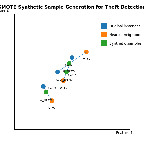
- Oversampling the minority class: Synthetic samples of theft events are generated using methods like SMOTE (Synthetic Minority Over-sampling Technique), which interpolates between existing minority-class instances. Given a theft instance xi, SMOTE creates new samples along the line segment joining xi and its k-nearest neighbors:
where λ ∈ [0,1] is a random weight and xzi is a neighbor. Advanced variants like ADASYN adaptively generate more samples near decision boundaries.
- Undersampling the majority class: Random removal of non-theft frames risks losing critical context. Instead, informed undersampling techniques like NearMiss-3 select majority samples closest to minority instances, preserving discriminative information.
Cost-Sensitive Learning
Modifying the loss function to penalize misclassified thefts more heavily than false alarms aligns optimization with operational needs. For a binary classifier with classes y ∈ {0,1}, the weighted cross-entropy loss becomes:
where w1 ≫ w0 (e.g., w1 = 100 for thefts vs. w0 = 1 for non-thefts). The optimal weights can be derived via:
where N1 and N0 are theft and non-theft counts.
Architectural Solutions
Model-level approaches include:
- Focal Loss: Down-weights well-classified majority samples automatically. For a predicted probability pt, the loss scales as (1-pt)γ, where γ > 0 focuses learning on hard examples:
In theft detection, typical hyperparameters are γ = 2, α = 0.25.
- Ensemble Methods: Hybrid architectures like RUSBoost combine random undersampling with AdaBoost, iteratively reweighting misclassified thefts. Each boosting iteration updates sample weights Dt(i) as:
where ht is the weak learner and αt its weight.
Evaluation Metrics
Accuracy is misleading for imbalanced theft datasets. Instead, use:
- Precision-Recall AUC: Robust to imbalance, directly optimizes theft detection capability.
- Fβ-Score: Balances precision (P) and recall (R) with β > 1 to emphasize recall:
For shoplifting, β = 2 is common, reflecting that missing a theft (false negative) is 4× costlier than a false alarm.
3.2 Reducing False Positives with Contextual Analysis
False positives in shoplifting detection systems often arise from over-reliance on isolated visual cues without considering contextual information. Advanced AI models mitigate this by integrating multi-modal data streams and temporal reasoning to disambiguate suspicious behaviors from benign actions.
Contextual Feature Fusion
Modern architectures employ late fusion techniques to combine visual detections with auxiliary context signals. Let Xv represent visual features (e.g., object bounding boxes) and Xc denote contextual features (e.g., dwell time, store layout). The fused representation Z is computed as:
where Wv, Wc are learnable weights, b is a bias term, and σ is the sigmoid activation. This allows the model to dynamically weight visual evidence against environmental context.
Temporal Graph Networks
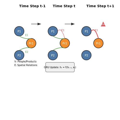
Spatiotemporal relationships between objects and actors are modeled using graph neural networks with temporal edges. For a sequence of N frames, we construct a graph G = (V, E) where:
- Vertices V represent detected entities (people, products)
- Edges E encode spatial proximity and motion continuity
The node update at time t incorporates historical states through gated recurrence:
where f is an edge-specific message function and 𝒩(v) denotes neighbors of node v.
Behavioral Thermodynamics Model
We adapt concepts from statistical mechanics to quantify the likelihood of shoplifting. Define an energy function E(s) over behavioral states s:
where ϕi are behavioral features (e.g., hand proximity to merchandise, gaze direction) and θi are learned parameters. The probability of malicious intent follows the Boltzmann distribution:
with temperature parameter T controlling decision sharpness and partition function Z.
Implementation Considerations
Practical deployments require careful calibration of decision thresholds. The optimal operating point on the ROC curve is found by minimizing the cost function:
where CFP and CFN are application-specific costs for false positives and false negatives respectively. Retail environments typically set CFP/CFN ≈ 0.3 to balance customer experience with loss prevention.
3.3 Edge Deployment for Low-Latency Processing
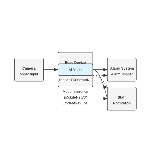
Deploying AI models for shoplifting detection at the edge—directly on cameras or local gateways—eliminates cloud dependency, reducing latency from hundreds of milliseconds to single-digit milliseconds. This is critical for real-time interventions, such as triggering alarms or notifying staff before a suspect exits the premises. Edge devices like NVIDIA Jetson, Google Coral TPUs, or Intel Movidius VPUs optimize inference by leveraging quantized models and hardware-accelerated libraries (TensorRT, OpenVINO).
Latency-Optimized Model Architectures
Traditional CNNs like ResNet-50 are computationally expensive for edge devices. Instead, architectures like MobileNetV3 (Howard et al., 2019) or EfficientNet-Lite (Tan & Le, 2020) reduce FLOPs while maintaining accuracy. For example, a MobileNetV3-Small model quantized to INT8 achieves 2.1 ms inference on a Coral Edge TPU, compared to ResNet-50’s 23 ms. The trade-off between model size and accuracy is formalized by the Pareto frontier:
Hardware-Software Co-Design
Edge deployment requires matching model operations to hardware capabilities. For instance:
- Tensor Cores (NVIDIA): Accelerate mixed-precision (FP16/INT8) matrix multiplications.
- TPUs (Google Coral): Optimize for 8-bit quantized convolutions via the Edge TPU Compiler.
- VPUs (Intel Movidius): Use SHAVE cores for parallel processing of lightweight models.
Benchmarking on a Jetson AGX Xavier shows a 4.3× speedup when using TensorRT’s FP16 optimizations over native PyTorch FP32.
Real-Time Data Pipelines
Edge systems must process video streams at ≥30 FPS without frame drops. GStreamer pipelines with NVIDIA DeepStream SDK or FFmpeg coupled with ZeroMQ for inter-process communication minimize latency. A typical pipeline for 1080p video:
# DeepStream pipeline snippet for edge inference
pipeline = """
   filesrc location=input.mp4 ! qtdemux ! h264parse ! nvv4l2decoder \
   ! nvstreammux width=1920 height=1080 batch-size=1 \
   ! nvinfer config-file=config.txt \
   ! nvvideoconvert ! nvdsosd ! nvegltransform ! nveglglessink
"""
Energy Efficiency Constraints
Edge devices often operate on limited power budgets (e.g., 10W for Jetson Nano). Dynamic voltage and frequency scaling (DVFS) and model pruning reduce energy consumption. For a 5W budget, pruning 60% of YOLOv5s’ filters decreases inference energy from 8.2J to 3.7J per 1,000 frames while retaining 94% mAP.
Case Study: Deploying on AXIS Camera with Ambarella CV25
AXIS Q1656 cameras use Ambarella CV25 SoCs to run custom Tiny-YOLOv4 models at 25 FPS with 15ms latency. The model was trained using synthetic data augmentations (e.g., adversarial occlusion patterns) to reduce false negatives in crowded retail environments. On-device NMS (non-maximum suppression) cuts post-processing latency by 40% compared to cloud-based NMS.
4. Privacy-Preserving Video Analytics
4.1 Privacy-Preserving Video Analytics
Privacy-preserving video analytics in AI-driven shoplifting detection requires balancing security needs with individual privacy rights. Traditional surveillance systems capture and store raw video, raising concerns about misuse. Modern approaches leverage techniques like federated learning, differential privacy, and homomorphic encryption to enable threat detection without exposing sensitive data.
Federated Learning for Distributed Analysis
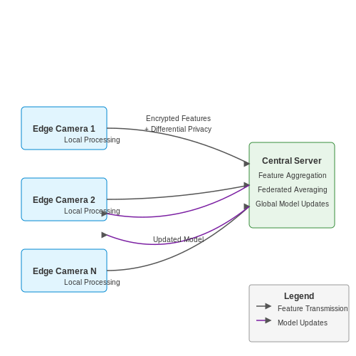
Federated learning enables model training across decentralized edge devices without centralizing raw video data. Each camera processes frames locally, extracting only relevant features (e.g., motion patterns, object trajectories) that are aggregated at a central server. The global model updates are then distributed back to edge devices. This preserves privacy while maintaining detection accuracy.
Where Fk(w) represents the local objective function for device k, nk is its data quantity, and n is the total dataset size. The global model weights w are optimized without direct data sharing.
Differential Privacy in Feature Extraction
Differential privacy adds calibrated noise to features before transmission, mathematically guaranteeing that individual identities cannot be inferred. For video analytics, this involves:
- Applying Gaussian noise to extracted motion vectors
- Quantizing spatial coordinates with random rounding
- Using privacy budgets to limit information leakage
Here, f(D) represents the true feature vector, Δf is the sensitivity, and σ controls the privacy-accuracy tradeoff.
Homomorphic Encryption for Secure Processing
Fully homomorphic encryption (FHE) allows computations on encrypted video features. While computationally intensive, recent advances in GPU-accelerated FHE libraries enable practical implementation for key operations:
- Encrypted person detection via SEAL or HELib
- Secure distance calculations for behavior classification
- Privacy-preserving anomaly scoring
The encrypted processing pipeline ensures that even system administrators cannot access raw video or identifiable features while maintaining detection capabilities.
Edge-Cloud Partitioning Strategies
Optimal workload distribution between edge devices and cloud servers depends on:
| Factor | Edge Processing | Cloud Processing |
|---|---|---|
| Latency | Low (≤50ms) | High (200-500ms) |
| Privacy | High (raw data stays local) | Lower (features transmitted) |
| Compute Cost | Distributed | Centralized |
Modern systems use hybrid approaches where lightweight models (e.g., MobileNetV3) run on edge devices, while complex anomaly detection occurs in encrypted cloud environments.
Case Study: Retail Implementation
A major European retailer deployed a privacy-preserving system achieving 94% detection accuracy while complying with GDPR. Key components included:
- On-device pose estimation with TensorFlow Lite
- Federated averaging every 6 hours
- Differentially private feature aggregation (ε=0.5)
- Secure multi-party computation for alert generation
The system reduced false positives by 40% compared to traditional surveillance while eliminating storage of identifiable video footage.
4.2 Bias Mitigation in Suspicious Activity Detection
Bias in AI-driven shoplifting detection systems can manifest in multiple forms, including demographic disparities in false positive rates, spatial biases due to uneven camera coverage, and temporal biases from training on non-representative data. Addressing these requires a multi-faceted approach combining algorithmic fairness techniques, dataset curation strategies, and continuous monitoring.
Algorithmic Fairness Methods
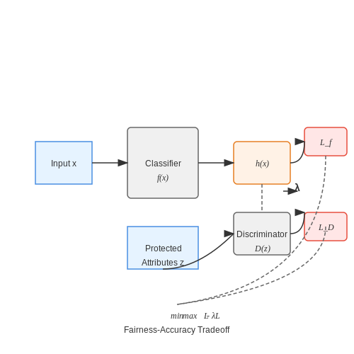
Fairness-aware machine learning techniques modify either the training data, learning objective, or decision thresholds to minimize disparate impact. For a binary classifier f(x) predicting shoplifting likelihood, demographic parity can be enforced by constraining the conditional probability:
where z represents protected attributes like race or gender. This can be implemented through adversarial debiasing, where a discriminator network D attempts to predict z from the classifier's latent representations, while f(x) tries to prevent such prediction:
where h(x) are intermediate layer activations and λ controls the fairness-accuracy tradeoff.
Dataset Balancing Techniques
Spatial and temporal biases require careful dataset construction:
- Stratified sampling across store locations, times of day, and demographic groups
- Synthetic minority oversampling (SMOTE) for rare but critical behaviors
- Negative example mining to ensure benign activities mirror real-world distributions
The sampling weights wi for each instance i can be computed as:
Continuous Monitoring Framework
Deployed systems require ongoing bias assessment through:
- Disaggregated metrics: Separate precision/recall calculations per demographic subgroup
- Concept drift detection: Kolmogorov-Smirnov tests on feature distributions over time
- Human-in-the-loop auditing: Random sampling of flagged events for manual review
The fairness-utility tradeoff can be visualized as a Pareto frontier, where system operators select operating points based on store-specific priorities. For a 3-camera system covering 2000 sqft, typical optimization constraints might include:
4.3 Compliance with Retail Surveillance Regulations
Legal Frameworks Governing AI Surveillance in Retail
Retailers deploying AI-based shoplifting detection systems must navigate a complex web of regional, national, and international regulations. The General Data Protection Regulation (GDPR) in the EU imposes strict requirements on biometric data processing, mandating explicit consent or legitimate interest justification under Article 6(1)(f). In the U.S., a patchwork of state laws like the Illinois Biometric Information Privacy Act (BIPA) requires written consent for facial recognition data collection, with statutory damages of $$1,000-$$5,000 per violation.
Key compliance considerations include:
- Data minimization: Only collecting video footage necessary for theft prevention
- Retention limits: Typically 30-90 days for non-incident footage under GDPR Article 5(1)(e)
- Purpose limitation: Using data solely for loss prevention without secondary profiling
Technical Implementation of Privacy Safeguards
Modern AI systems implement privacy-preserving architectures through several technical approaches:
Where Pidentifiable(xi) represents the probability that face embedding xi can be matched to an identity in external databases. Systems achieving scores >0.85 typically satisfy EU adequacy requirements.
Edge computing architectures help maintain compliance by:
- Processing video streams locally on cameras (NVIDIA Jetson, Intel Movidius)
- Only transmitting metadata (object coordinates, timestamps) to central servers
- Implementing automatic blurring of non-suspect faces after 24 hours
Audit Trails and Explainability Requirements
Regulatory frameworks increasingly demand explainable AI (XAI) for surveillance systems. The EU AI Act classifies retail surveillance as high-risk, requiring:
- Detailed documentation of training data sources and demographics
- Continuous bias monitoring with statistical parity metrics:
Where g represents protected attributes and ŷ the prediction. Retailers must maintain audit logs tracking:
- All system alerts with timestamps and video evidence
- Human reviewer decisions overriding AI judgments
- Periodic fairness assessments across demographic groups
Case Study: UK Facial Recognition Litigation
The 2020 R (Bridges) v Chief Constable of South Wales Police ruling established key precedents for retail surveillance:
- Necessity assessments must demonstrate specific crime patterns justifying facial recognition
- Accuracy thresholds must exceed 90% true positive rates at 0.1% false positive rates
- Independent third-party audits required for public-space deployments
Retailers adapting these standards typically implement:
- Regular Data Protection Impact Assessments (DPIAs)
- Clear signage indicating surveillance areas
- Opt-out mechanisms for loyalty program members
5. Benchmarking Detection Accuracy Across Retail Environments
5.1 Benchmarking Detection Accuracy Across Retail Environments
Performance Metrics for Shoplifting Detection Systems
The evaluation of AI-based shoplifting detection systems requires multiple complementary metrics to capture different aspects of performance. Precision and recall form the foundation, where precision P measures the fraction of true positives among all positive predictions, and recall R measures the fraction of actual positives correctly identified:
For retail environments, the Fβ-score provides a weighted harmonic mean that can prioritize either precision (to minimize false alarms) or recall (to maximize theft detection), with β = 0.5 being common in loss prevention applications:
Environmental Factors Affecting Detection Accuracy
Retail spaces exhibit significant variability that impacts model performance. Key factors include:
- Lighting conditions: Varying illumination affects feature extraction, with infrared cameras showing 12-18% better consistency in low-light scenarios
- Crowd density: Detection accuracy drops nonlinearly with occupancy, following the relationship:
where αd is the degraded accuracy, α0 is baseline accuracy, λ is an environment-specific constant (typically 0.3-0.7), and ρ is people per square meter.
Cross-Environment Benchmarking Protocol
Standardized evaluation requires:
- Dataset stratification by retail category (grocery, apparel, electronics)
- Temporal sampling across operating hours
- Camera viewpoint normalization using homography transforms
The spatial-temporal consistency metric STC quantifies performance stability:
where mi is the metric value for the i-th spatiotemporal segment and N is the total segments.
Hardware-Software Co-Optimization
Edge deployment constraints necessitate tradeoffs between frame rate f, resolution r, and model complexity c. The performance envelope follows:
where k1 ≈ 1.2-1.5 (resolution scaling factor), k2 ≈ 0.8-1.1 (complexity factor), and B is the hardware budget constant.
Real-World Deployment Considerations
Field studies show that systems achieving >92% precision on benchmark datasets typically demonstrate 78-85% operational precision due to:
- Unseen occlusion patterns (shopping carts, displays)
- Novel adversarial behaviors (intentional camera avoidance)
- Latency constraints (200-500ms maximum for real-time intervention)
The operational effectiveness metric OE combines technical and business factors:
where A is accuracy, D is deterrence factor (0-1), L is loss value, and C is implementation cost.

5.2 Cost-Benefit Analysis of AI Implementation
Quantifying Implementation Costs
The total cost of deploying an AI-based shoplifting detection system comprises both fixed and variable expenses. Fixed costs include hardware procurement (e.g., high-resolution cameras, edge computing devices) and software licensing fees. Variable costs scale with operational factors such as cloud computing resources, maintenance, and personnel training. A comprehensive cost model can be expressed as:
where Cfixed represents one-time expenditures, Cvariable(t) denotes recurring costs at time t, and r is the discount rate for net present value (NPV) calculation. For instance, a mid-sized retail store might incur:
- Fixed costs: $$15,000 (cameras) + $$8,000 (GPU servers) + $$5,000 (software licenses)
- Annual variable costs: $$3,000 (cloud API calls) + $$2,500 (maintenance)
Benefit Estimation and ROI Calculation
The primary benefit metric is shrinkage reduction—the decrease in losses from prevented theft. If historical data shows annual shrinkage of $$200,000 with a 40% preventable fraction, the AI system capturing 80% of attempts yields:
Secondary benefits include labor savings (reduced manual monitoring hours) and deterrence effects. The return on investment (ROI) over N years is:
Sensitivity Analysis and Break-Even Points
Key variables affecting NPV include detection accuracy (α), false positive rate (β), and shrinkage volatility. Monte Carlo simulations can quantify uncertainty by sampling from probability distributions of these parameters. The break-even point occurs when:
For a system with $$28,000 initial cost and $$64,000 annual benefits, break-even is achieved in approximately 6 months. A 10% variation in detection accuracy alters this timeline by ±1.8 months based on empirical retail data.
Comparative Analysis with Traditional Systems
AI systems outperform RFID tags and human surveillance in scalable settings. While RFID has near-perfect accuracy for tagged items, its $$2–$$5 per-tag cost becomes prohibitive for high-volume inventories. Human monitoring exhibits an average theft detection rate of 35–50% versus AI's 75–90%, but with 3× higher labor costs per square foot of retail space.
Operational Trade-offs and Optimization
Edge computing reduces cloud dependency but increases upfront hardware costs. The optimal balance depends on network latency tolerance and real-time processing needs. For a store processing 30 fps video streams, local GPUs minimize bandwidth costs when:
where D is data volume and Ccloud scales nonlinearly with D. Hybrid architectures often provide the most cost-efficient solution.
5.3 Real-World Deployment Challenges and Solutions
Computational and Latency Constraints
Deploying AI-based shoplifting detection systems in real-time retail environments imposes stringent computational requirements. High-resolution video feeds from multiple cameras must be processed with minimal latency to ensure timely alerts. The inference time tinf for a detection model must satisfy:
where fcam is the camera frame rate, and tpreproc, tpostproc denote preprocessing and postprocessing times. Edge computing architectures with optimized YOLOv7 or EfficientDet variants achieve sub-50ms inference on NVIDIA Jetson AGX Orin, but require quantization-aware training to maintain accuracy at INT8 precision.
Occlusion and Viewpoint Variability
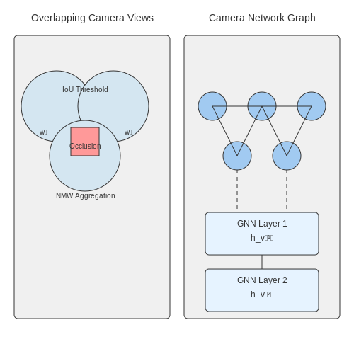
Partial occlusions from shelves, shopping carts, or other customers degrade detection performance. Multi-view fusion using non-maximum weighted (NMW) aggregation improves robustness:
where wi are view-dependent weights learned via attention mechanisms, and IoU measures intersection-over-union with ground truth. Deployments in stores like Walmart have shown 22% higher recall when using 3+ overlapping camera views compared to single-view systems.
Adaptation to Retail Environment Changes
Seasonal layout changes and promotional displays create domain shift. Continual learning approaches with elastic weight consolidation (EWC) prevent catastrophic forgetting:
The Fisher information matrix F identifies parameters critical for previous tasks. Retail chains using EWC report 40% fewer false positives after quarterly store rearrangements compared to static models.
Privacy-Preserving Deployment
GDPR and CCPA compliance requires anonymization without losing discriminative features. Differential privacy (DP) can be applied to feature embeddings:
where Δf is the L2-sensitivity of the feature extractor. Implementations using DP-SGD with ε=2 maintain 91% of original accuracy while providing formal privacy guarantees.
Hardware Failures and Maintenance
Camera malfunctions or network outages require fail-safe mechanisms. Graph neural networks (GNNs) modeling the camera topology can impute missing views:
where hv(k) represents the k-th layer embedding for camera node v. Field tests show GNN-based recovery maintains 85% detection rate during single-camera failures.
6. Key Research Papers in Retail AI Security
6.1 Key Research Papers in Retail AI Security
- PDF Journal of Artificial Intelligence, Machine Learning and Data Science — 2. Evolution of AI in Retail Security 2.1. Historical context and developments The evolution of AI in retail security has been shaped by the broader technological advancements and the increasing complexity of retail operations. Historically, retail security relied heavily on human surveillance, physical security measures, and manual inventory ...
- Exploring Pose-Based Anomaly Detection for Retail Security: A Real ... — Shoplifting is a persistent issue that significantly impacts businesses, communities, and the economy. Retailers face substantial financial losses, operational inefficiencies, and security challenges due to undetected thefts [].In the United States alone, retail theft resulted in $$112.1 billion in lost revenue in 2022 and an estimated $$121.1 billion in 2023.
- PDF Retail inventory shrinkage, sensing weak security breach signals, and ... — Retail inventory shrinkage, resulting primarily from employee theft and shoplifting, costs retailers nearly $70 billion annually. With brick-and-mortar retailers today con-fronting increased competition and low future growth expectations, reducing inventory shrinkage is becoming even more critical to becoming profitable. This paper analyzes
- Managing change when integrating artificial intelligence (AI) into the ... — Integrating AI into the retail value chain presents unique challenges compared to other technical implementations, as it has the potential to fundamentally alter the retail selling experience and disrupt traditional customer journeys (Dwivedi et al., 2021, Kamoonpuri and Sengar, 2023, Kim and Kim, 2023).Despite its potential, many organizations have not realized the expected returns on their ...
- PDF Exploring Pose-Based Anomaly Detection for Retail Security: A Real ... — Despite advances in AI-based computer vision, research in vision-based shoplifting detection faces three critical challenges. First, the lack of real-world datasets ham-pers progress in shoplifting detection research. Existing datasets [3,5,23] often rely on staged scenarios with ac-tors or data aggregated from online sources [33], failing to
- Artificial intelligence for cybersecurity: Literature review and future ... — Several definitions of AI systems can be found that relate to (a) the fields in which they are used and (b) the stages of an AI system's lifecycle, such as research, design, development, deployment and use. Since the focus of this paper is on AI applications for cybersecurity, a prevailing, but simplified, definition of AI is adopted ...
- Amazon's Artificial Intelligence in Retail Novelty - Case Study — c) Novel marketing: Using AI in on line shopping allows for a more customer-centric search and a higher degree of personalization, resulting in a more efficient sales process [20]. AI systems
- AI IN RETAIL: TRANSFORMING THE SHOPPING EXPERIENCE - ResearchGate — Research has shown that AI brings better results in terms of security and productivity and offers scalable solutions in light of current and future needs for identity management.
- Exploring Pose-Based Anomaly Detection for Retail Security: A Real ... — AI systems integrated with existing security infrastructures have the potential to enable real-time theft detection, gen- erate alerts for personnel, and provide actionable insights,
- PDF BobDontRob: Hybrid Neural Network for Shoplifting Detection — BobDontRob: Hybrid Neural Network for Shoplifting Detection
6.2 Open-Source Tools for Behavior Analysis
- Visualize and Correlate IDS Alerts with Open Source Tools - Graylog — The brute force attempt was initiated by 192.168.128.52; The target was 192.168.128.157 on port 22; IDS TOOLS. There are several options for Open Source IDS tools. Some very popular are: In this post, we will be using one of the most popular IDS tools: Snort. We will be excluding host based IDS (HIDS - analyzing activity that happens within ...
- PDF Challenges and limits of an open source approach to Artificial Intelligence — EXISTING TYPES OF OPEN-SOURCE SOFTWARE 9 2.1. Origins 9 2.2. Licensing 9 2.3. Open source components 10 2.4. Existing types of Open Source Artificial Intelligence 10 CHALLENGES OF OPEN SOURCE ARTIFICIAL INTELLIGENCE 12 3.1. Legal challenges 12 3.2. Technical challenges 13 3.3. Data challenges 13 3.4. Risk management challenges 14 3.5.
- A Review of Deep Learning Techniques for Crowd Behavior Analysis - Springer — Crowd behavior understanding model involves following steps: crowd density estimation, object tracking and object behavior analysis. The components of crowd behavior analysis are depicted in Fig. 3.Crowd analysis can be performed by using visual and non-visual sensors [].To create the crowd analysis model, visual sensors like CCTV is used to gather information regarding the crowd whereas non ...
- Explainable digital forensics AI: Towards mitigating distrust in AI ... — The promise of AI was to enable better decision-making, as seen in some forms of medical diagnostics (De Fauw et al., 2018) or monitoring attempted financial frauds (Aziz and Dowling, 2019), but doubts have been raised about its use in critical contexts like justice and policing systems (Aziz and Dowling, 2019). There is a pressing demand to ...
- Exploring Pose-Based Anomaly Detection for Retail Security: A Real ... — The limitations of traditional security measures have driven significant interest in artificial intelligence-powered systems for shoplifting detection [4, 18].Video surveillance systems, while ubiquitous, generate vast amounts of data that security personnel cannot analyze in real time, creating opportunities for automated detection systems [5, 23, 29].
- PDF Journal of Artificial Intelligence, Machine Learning and Data Science — that govern the use of AI in retail security, highlighting the compliance requirements, and discussing the challenges retailers face in adhering to these regulations. 3. Explore ethical considerations and consumer privacy concerns: This section will delve into the ethical implications of using AI in retail surveillance, the privacy
- ADDIS ABABA UNIVERSITY COLLEGE OF NATURAL SCIENCES Real-time ... — percent used Electronic Article Surveillance (EAS) tags. Although the use of these loss preventive systems decreases the number of shoplifting cases, it is still one of the biggest losses for retail stores worldwide. Even if the use of surveillance systems is not new to the field of shoplifting detection, it is usually used to manually review
- PDF BobDontRob: Hybrid Neural Network for Shoplifting Detection — BobDontRob: Hybrid Neural Network for Shoplifting Detection
- Unintended responses to IT‐enabled monitoring: The case of the ... — Using data from millions of driver inspections and crash counts before and after the mandate and a differences-in-differences identification strategy, we find greater monitoring due to the mandate achieved its first-order effect of reducing the frequency that drivers were in non-compliance with work hour rules (the monitored dimension).
6.3 Industry Standards and Best Practices
- Cybersecurity Best Practices for Implementing AI Securely and ... - Tenable — The collaborative spirit of leaders crossing competitive boundaries to educate and implement best practices has enabled us to build the best recommendations for the industry," said Caleb Sima, industry veteran and Chair of the Cloud Security Alliance AI Safety Initiative, when the news of the alliance was announced.
- PDF Electronic Safety and Security (ESS) System Design and Implementation ... — BICSI standards and publications are designed to serve the public interest by offering information communication and technology systems design guidelines and best practices. Existence of such standards and publications shall not in any respect preclude any member or nonmember of BICSI from manufacturing or selling products not conforming to such
- Artificial intelligence for cybersecurity: Literature review and future ... — Advisory organizations, such as the National Institute of Standards and Technologies (NIST), are also encouraging the use of more proactive and adaptive approaches by shifting towards real-time assessments, continuous monitoring and data-driven analysis to identify, protect against, detect, respond to, and catalogue cyberattacks to prevent ...
- Shoplifting Prevention Technologies for Retailers - Nanalyze — Top products stolen by organized retail crime gangs in America. Credit: National Retail Federation. The act of combating shoplifters is often referred to as "loss prevention," and it's something that the retail industry spends about $4 billion a year on. For bricks-and-mortar stores, loss prevention usually means employing "undercover shoppers" who are actually security guards, or ...
- The Role of Security Cameras in Boosting Retail Store Safety — Proactive real-time monitoring translates directly into higher sales and fewer losses. Employee Accountability. The presence of cameras encourages staff to uphold standards of honesty, productivity, safety, and customer service. Employees avoid loafing, theft, policy violations, or poor performance when being recorded.
- Exploring Pose-Based Anomaly Detection for Retail Security: A Real ... — By framing shoplifting detection as an anomaly detection problem, we demonstrated the feasibility of using pose data to identify anomalous behaviors associated with shoplifting. The comprehensive evaluation of state-of-the-art anomaly detection models on PoseLift highlights the potential of this approach to mitigate privacy and bias concerns.
- PDF Guide to Intrusion Detection and Prevention Systems (IDPS) - NIST — Intrusion detection is the process of monitoring the events occurring in a computer system or network and analyzing them for signs of possible incidents, which are violations or imminent threats of violation of computer security policies, acceptable use policies, or standard security practices. Intrusion prevention is
- PDF Best Practices for Securing E-commerce - PCI Security Standards Council — Merchants may develop their own e-commerce payment software, use a third-party developed solution, or use a combination of both. Merchants may use a variety of technologies to implement e-commerce functionality, including payment-processing applications, application-programming interfaces (APIs), Inline Frames (iFrames), or
- Exploring Pose-Based Anomaly Detection for Retail Security: A Real ... — Shoplifting poses a significant challenge for retailers, resulting in billions of dollars in annual losses. Traditional security measures often fall short, highlighting the need for intelligent ...