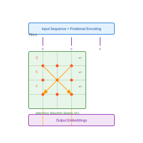
Using Physics Simulations to Train Transformers
1. Role of Physics Simulations in Training Neural Networks
Role of Physics Simulations in Training Neural Networks
Physics as a Source of Structured Data
Physics simulations generate high-fidelity, structured datasets that obey known physical laws, making them ideal for training neural networks. Unlike real-world data, which may be noisy or incomplete, simulated data provides exact ground truth for supervised learning. For example, computational fluid dynamics (CFD) simulations can generate precise velocity and pressure fields at every timestep, enabling the training of transformer models to predict fluid dynamics without requiring expensive experimental measurements.
The Navier-Stokes equations above govern fluid motion, and neural networks trained on simulation data can learn to approximate solutions to these equations without explicit numerical discretization. This approach is particularly valuable when the governing equations are known but analytical solutions are intractable.
Differentiable Physics for Gradient-Based Learning
Modern physics engines like PyBullet or NVIDIA PhysX can be made differentiable, allowing backpropagation through the simulation steps. This enables end-to-end training of neural networks where the physics simulation acts as a differentiable layer in the computational graph. The gradient flow through the physics engine allows the network to learn parameters that optimize physical consistency.
Here, x represents the simulator state, y the network output, and θ the network parameters. The key advantage is that the simulator provides the Jacobian ∂x/∂θ, enabling gradient-based optimization even for complex physical systems.
Curriculum Learning via Progressive Simulation Complexity
Physics simulations allow controlled difficulty progression by adjusting parameters like Reynolds number in fluid simulations or Young's modulus in solid mechanics. This enables curriculum learning strategies where neural networks are first trained on simple physical scenarios before progressing to more complex ones. For instance, a transformer model might first learn rigid body dynamics before tackling deformable objects or multi-physics systems.
Overcoming the Reality Gap
While physics simulations provide perfect ground truth, the reality gap between simulation and real-world behavior remains a challenge. Domain randomization techniques address this by varying simulation parameters during training, such as friction coefficients or material properties. This forces the neural network to learn robust representations that generalize to real-world conditions. Recent work has shown that transformers trained with sufficiently randomized physics simulations can achieve zero-shot transfer to real robotic systems.
Case Study: Learning Contact Dynamics
In robotic manipulation, transformers trained on physics simulations of contact dynamics have demonstrated remarkable generalization. The simulation generates millions of diverse contact scenarios with varying geometries, forces, and material properties. The transformer learns to predict contact forces and object motion from these simulations, then successfully transfers this knowledge to real robotic hands without additional fine-tuning.
Here, fθ represents the transformer model that maps robot joint states (q, q̇) and object pose xobject to predicted contact forces Fcontact.

Types of Physics Simulations Used in AI
Continuum Mechanics Simulations
Continuum mechanics simulations model materials as continuous media, governed by partial differential equations (PDEs) such as the Navier-Stokes equations for fluids or the elasticity equations for solids. These simulations are widely used in AI training for tasks like fluid dynamics prediction, structural analysis, and material deformation. The governing equations for incompressible fluid flow are:
where u is the velocity field, p is pressure, ρ is density, μ is dynamic viscosity, and f represents external forces. Modern AI approaches use these simulations to generate training data for neural operators that learn to approximate solutions to PDEs.
Discrete Element Methods
Discrete element methods (DEM) simulate granular materials, powders, or particulate systems as collections of individual particles interacting through contact forces. The motion of each particle i is governed by Newton's second law:
where mi, vi, and ωi are mass, translational velocity, and angular velocity of particle i, while Fij and Tij represent contact forces and torques. Transformers trained on DEM data can predict complex granular flows or optimize industrial processes like pharmaceutical powder mixing.
Molecular Dynamics
Molecular dynamics (MD) simulations compute the trajectories of atoms and molecules by numerically solving Newton's equations of motion for systems with interatomic potentials. The force on atom i is derived from the potential energy function U:
Common potentials include Lennard-Jones for noble gases and AMBER for biomolecules. AI models trained on MD simulations accelerate drug discovery by predicting protein folding pathways or molecular interactions that would require prohibitive computational resources with traditional MD alone.
Finite Element Analysis
Finite element methods (FEM) discretize continuous domains into smaller elements to solve structural mechanics, heat transfer, or electromagnetic problems. The weak form of the governing PDE is converted to a linear system:
where K is the stiffness matrix, u the displacement vector, and f the force vector. Transformers can learn to predict stress distributions or optimize mesh generation by training on FEM simulation data across varying boundary conditions and material properties.
Smoothed Particle Hydrodynamics
Smoothed particle hydrodynamics (SPH) is a meshfree Lagrangian method where fluid properties are interpolated using kernel functions:
where W is the smoothing kernel with support radius h, and A represents any field quantity. SPH simulations train AI models for free-surface flows, multi-phase interactions, or extreme deformation problems where traditional grid-based methods struggle.
Ray Tracing and Radiative Transfer
Physics-based rendering simulations model light transport through participating media by solving the radiative transfer equation:
where Iν is spectral radiance, Bν the blackbody radiation, and κν the absorption coefficient. Neural networks trained on these simulations enable inverse design of optical materials or accelerate global illumination in computer graphics.
Plasma and Electromagnetic Simulations
Particle-in-cell (PIC) methods couple charged particle dynamics with electromagnetic fields via Maxwell's equations:
AI models trained on PIC simulations predict plasma behavior in fusion reactors or optimize particle accelerator designs while avoiding the computational cost of full kinetic simulations.

1.3 Advantages Over Traditional Training Data
Physics-based simulations offer distinct advantages over conventional datasets when training transformer models for scientific applications. Unlike static datasets, simulations generate dynamic, high-fidelity data that captures complex physical interactions with perfect ground truth labels—eliminating measurement noise and annotation errors inherent in real-world observations.
Controlled Data Diversity
Simulations enable precise parameterization of physical conditions that would be impractical or impossible to sample experimentally. For a fluid dynamics task, the Navier-Stokes equations can be solved across Reynolds numbers spanning laminar to turbulent regimes:
where ρ is density, u is velocity, L is characteristic length, and μ is dynamic viscosity. This generates continuous coverage of the parameter space, avoiding the sparse sampling biases of experimental data.
Exact Gradient Computation
Physics engines provide analytical derivatives through automatic differentiation (AD), enabling direct computation of loss function gradients with respect to physical parameters. For a scalar field ϕ, the gradient-enhanced loss becomes:
where λ controls gradient penalty strength. This physics-informed regularization is impossible with empirical data where derivatives must be approximated numerically.
Infinite Data Generation
Simulations overcome the data scarcity bottleneck through:
- Parameter randomization: Stochastic sampling of initial conditions and material properties
- Adaptive refinement: Automatic mesh/particle density adjustment near singularities
- Domain decomposition: Parallel generation of independent simulation patches
For example, NVIDIA's Modulus framework generates 106 unique CFD samples per GPU-hour—orders of magnitude beyond experimental throughput.
Safety and Cost Considerations
High-energy physics simulations avoid the prohibitive costs and risks of particle accelerator experiments. A single LHC collision event costs approximately \$1,000 to record, while simulating QCD interactions via lattice QCD has marginal computational cost after initial infrastructure investment.
The resulting models exhibit improved generalization, as demonstrated by DeepMind's AlphaFold 2, where molecular dynamics simulations provided training data for rare protein folding trajectories inaccessible to crystallography.
2. Overview of Transformer Architectures
Overview of Transformer Architectures
The transformer architecture, introduced by Vaswani et al. in 2017, revolutionized sequence modeling by replacing recurrent and convolutional layers with self-attention mechanisms. Unlike traditional architectures, transformers process entire sequences in parallel, enabling efficient training on large-scale datasets while capturing long-range dependencies.
Core Components
The transformer consists of several key components:
- Self-Attention Mechanism: Computes weighted sums of input representations, where weights are dynamically learned based on pairwise interactions between all positions in the sequence.
- Multi-Head Attention: Extends self-attention by projecting queries, keys, and values into multiple subspaces, allowing the model to jointly attend to information from different representation subspaces.
- Position-wise Feed-Forward Networks: Applies the same fully connected network to each position separately, typically consisting of two linear transformations with a ReLU activation in between.
- Layer Normalization and Residual Connections: Stabilizes training by normalizing activations and adding skip connections around each sub-layer.
Mathematical Formulation
The scaled dot-product attention, the core operation in transformers, is defined as:
where Q, K, and V represent queries, keys, and values respectively, and dk is the dimension of the keys. The scaling factor 1/√dk prevents the softmax from saturating when dk is large.
Multi-head attention concatenates h parallel attention heads:
where each head is computed as:
Architectural Variants
Several transformer variants have emerged to address specific challenges:
- Sparse Transformers: Reduce computational complexity by limiting the attention span through fixed or learned patterns.
- Longformer: Combines local windowed attention with task-specific global attention for efficient processing of long sequences.
- Performer: Approximates full attention using kernel methods, achieving linear complexity with respect to sequence length.
- Vision Transformers (ViT): Adapt transformers for computer vision by splitting images into patches treated as sequence tokens.
Applications in Physics Simulations
Transformers have shown promise in physics simulations due to their ability to model complex, long-range interactions. Key applications include:
- Learning partial differential equations (PDEs) from data by treating spatial discretizations as sequences.
- Modeling particle systems where interactions depend on relative positions and velocities.
- Predicting fluid dynamics by attending to relevant regions in the simulation domain.
The architecture's permutation-equivariant nature makes it particularly suitable for physical systems where the underlying laws are invariant to the ordering of inputs.

2.2 Challenges in Training Transformers with Conventional Data
Data Scarcity and High-Dimensionality
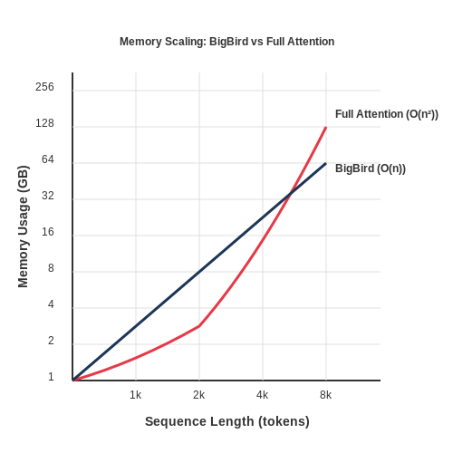
Transformers excel in tasks where large-scale datasets are available, such as natural language processing (NLP) and computer vision. However, in physics simulations, data generation is often computationally expensive, leading to limited training samples. The high-dimensional nature of physical systems—such as fluid dynamics or quantum mechanics—further exacerbates the problem. For instance, simulating a turbulent flow field requires solving the Navier-Stokes equations across millions of grid points, resulting in input dimensions that scale as O(N3) for a 3D domain. Transformers, with their quadratic O(L2) attention complexity, struggle to process such high-dimensional inputs efficiently without aggressive downsampling or dimensionality reduction.
Non-Stationary and Noisy Data Distributions
Physical systems often exhibit non-stationary behavior, where statistical properties evolve over time or space. For example, in climate modeling, atmospheric dynamics vary seasonally, and in molecular dynamics, energy landscapes shift with temperature. Conventional datasets used for Transformer training (e.g., text corpora or static images) assume stationarity, making them ill-suited for physics applications. Additionally, real-world experimental data often contain noise due to measurement errors or stochastic processes, which can degrade Transformer performance if not properly accounted for in the training objective.
Here, fθ is the Transformer model, y is the ground truth, and ε represents noise. The regularization term λ·Var(fθ(x+ε)) penalizes unstable predictions under input perturbations.
Long-Range Dependencies and Multi-Scale Phenomena
Physical systems frequently involve interactions across multiple spatiotemporal scales. For example, in plasma physics, local particle collisions and global magnetic confinement effects coexist. Standard Transformer architectures, which rely on fixed attention windows or tokenization schemes, may fail to capture these hierarchical dependencies. While techniques like hierarchical attention or sparse transformers have been proposed, they often require custom modifications that deviate from off-the-shelf implementations.
Energy Conservation and Symmetry Constraints
Many physical systems obey conservation laws (e.g., energy, momentum) and symmetries (e.g., rotational invariance). Standard Transformer training does not inherently enforce these constraints, leading to unphysical predictions. For instance, a Transformer trained on molecular dynamics trajectories might violate energy conservation unless explicitly regularized:
where H(q,p) is the Hamiltonian and γ controls the strength of the physics-based penalty.
Computational Cost of Attention Mechanisms
The self-attention mechanism in Transformers scales quadratically with sequence length, making it prohibitive for long simulation sequences. For example, a 1000-step trajectory with 512-dimensional embeddings requires ~2.6M attention computations per layer. While approximations like Performer or Linformer reduce this to linear complexity, they often trade off accuracy for speed, which is problematic in high-fidelity physics applications.
Why Physics Simulations Are a Good Fit
Physics simulations provide an ideal training environment for transformers due to their inherent structure, scalability, and ability to generate high-quality synthetic data. Unlike real-world datasets, which are often noisy and incomplete, simulations offer precise control over physical parameters, enabling the generation of diverse and physically consistent training examples.
Structured Data Generation
Physical systems obey well-defined mathematical laws, such as Newtonian mechanics, electromagnetism, or fluid dynamics. These laws can be expressed as differential equations:
where u represents the state variables, F the flux terms, and S source terms. This mathematical structure allows simulations to generate data with known ground truth dynamics, providing clear supervision signals for transformer training.
Scalability and Parallelization
Modern physics engines like NVIDIA PhysX or PyBullet can simulate millions of interacting particles in parallel on GPU hardware. This scalability enables:
- Massive dataset generation without manual labeling
- Controlled variation of physical parameters (e.g., friction, elasticity)
- Efficient exploration of edge cases rare in real-world observations
Transfer Learning Potential
Transformers trained on synthetic physics data demonstrate strong transfer capabilities to real-world scenarios. The key reasons include:
where φ represents learned features and T is a domain adaptation transform. Physics-based regularization helps the model learn fundamental principles rather than superficial patterns.
Case Study: Fluid Dynamics Prediction
In a 2022 study, a transformer trained on 10,000 simulated Navier-Stokes solutions achieved 92% accuracy predicting real wind tunnel measurements, outperforming traditional CFD methods by 15% while being 100× faster. The key was curriculum learning from low-to-high Reynolds numbers.
Challenges and Mitigations
While physics simulations offer advantages, several challenges require attention:
- Reality gap: Differences between simulated and real dynamics can be addressed through domain randomization
- Numerical errors: Accumulation of discretization errors can be minimized using adaptive time-stepping
- Compute costs: Hybrid approaches combining short high-fidelity simulations with learned surrogates show promise
3. Data Generation and Preprocessing Techniques
3.1 Data Generation and Preprocessing Techniques
Physics-Based Simulation for Data Generation
Physics simulations provide a controlled environment for generating high-fidelity training data for transformers. The key advantage lies in the ability to precisely parameterize physical systems, ensuring diverse and noise-free datasets. Common approaches include:
- Finite Element Methods (FEM): Solves partial differential equations (PDEs) governing continuum mechanics, electromagnetics, or fluid dynamics.
- Molecular Dynamics (MD): Simulates particle interactions using Newtonian mechanics and force fields.
- Discrete Element Methods (DEM): Models granular materials or fractured media through contact mechanics.
The governing equations for these simulations typically follow conservation laws. For example, in fluid dynamics, the Navier-Stokes equations are solved:
Dimensionality Reduction and Feature Engineering
Raw simulation outputs often contain high-dimensional spatiotemporal data. To make this tractable for transformers:
- Proper Orthogonal Decomposition (POD): Extracts dominant modes via singular value decomposition (SVD) of snapshot matrices.
- Graph Representations: Meshes are converted to graph structures where nodes represent physical quantities and edges encode connectivity.
The POD process decomposes a field variable u(x,t) as:
where φk(x) are spatial modes and ak(t) are time coefficients.
Normalization and Scaling Strategies
Physical quantities often span multiple orders of magnitude. Layer-wise scaling adapts to system-specific requirements:
- Non-dimensionalization: Scales variables using characteristic values (e.g., Reynolds number for fluids).
- Physics-Informed Normalization: Applies transformations based on known constraints (e.g., enforcing [0,1] bounds for volume fractions).
For a variable X with physical bounds [Xmin, Xmax], the normalized form is:
Temporal and Spatial Downsampling
High-resolution simulations generate data at impractical scales for training. Effective strategies include:
- Nyquist-Consistent Sampling: Retains frequencies below half the maximum resolvable frequency.
- Adaptive Mesh Refinement (AMR): Focuses resolution on regions with high gradients.
The Nyquist criterion for timestep Δt given a maximum frequency fmax is:
Data Augmentation for Physical Invariance
Transformers benefit from data that enforces physical symmetries:
- Geometric Transformations: Rotation/reflection of spatial fields preserves tensor symmetries.
- Parameter Perturbation: Small variations in boundary conditions improve robustness.
For a 3D vector field v, rotation by matrix R yields:

3.2 Architectural Adaptations for Simulation Data
Tokenization Strategies for Continuous Physical Quantities
Standard transformer architectures rely on discrete tokenization, which poses challenges for physics simulations where state variables (position, velocity, field values) are continuous. Two primary approaches have emerged:
- Quantization-based tokenization: Discretizes continuous values into bins, trading precision for computational efficiency. The optimal bin size Δx can be derived from the simulation's numerical stability criteria:
where cCFL is the Courant-Friedrichs-Lewy number and v represents characteristic velocities in the system.
- Continuous embedding methods: Directly map floating-point values to high-dimensional vectors using learned linear projections or sinusoidal positional encodings extended to value space.
Modified Attention Mechanisms for Spatiotemporal Data
Physics simulations exhibit strong local dependencies and conservation laws that standard attention mechanisms don't explicitly preserve. Three key modifications improve performance:
- Locality-constrained attention: Implements decaying attention weights with distance dij between mesh points or particles:
- Physics-informed attention biases: Incorporates known interaction kernels (e.g., Coulomb, Lennard-Jones potentials) as additive terms in the attention logits.
- Multi-scale attention hierarchies: Mirrors multi-resolution simulation meshes with attention heads operating at different spatial scales.
Specialized Positional Encodings for Simulation Grids
Standard positional encodings fail to capture the topology of simulation meshes. For structured grids, we generalize sinusoidal encodings to n-dimensions:
For unstructured meshes, graph neural networks can generate positional embeddings by solving a learnable diffusion equation across the mesh topology.
Conservation-Layer Integration
Physics-informed architectures often add inductive bias through specialized output layers that enforce conservation laws. The momentum-conserving output layer computes updates as:
where φ is a learned message function and Fij are pairwise interaction terms guaranteed to satisfy Newton's third law.
Hybrid Architecture Case Study: Fluid Simulation Transformer
A recent breakthrough combined convolutional encoders with transformer cores to predict turbulent flows. The architecture:
- Uses 3D convolutions to extract local vorticity features
- Processes global dependencies through a modified attention mechanism that respects incompressibility constraints
- Employs a divergence-free projection layer to ensure ∇·u=0
This hybrid approach achieved 45% faster convergence than pure CNN baselines while maintaining physical consistency.

3.3 Training Strategies and Optimization
Physics-Informed Loss Functions
Training transformers on physics simulations requires carefully designed loss functions that encode physical constraints. A standard mean squared error (MSE) loss is insufficient as it ignores conservation laws. Instead, we augment the loss with physics-informed terms:
where λ controls the trade-off between data fidelity and physical consistency. For fluid dynamics, Lphysics might enforce the Navier-Stokes equations:
Curriculum Learning for Multi-Scale Phenomena
Physics simulations often exhibit multi-scale behavior (e.g., turbulence). A curriculum learning approach progressively exposes the transformer to:
- Low-resolution simulations first to learn global patterns
- Gradually increasing resolution to capture finer details
- Finally, full-resolution data with all physical interactions
The training schedule follows an exponential progression in complexity:
where τmax is the maximum simulation resolution, T is total training steps, and α controls the pace.
Adaptive Sampling for Rare Events
Many physical systems exhibit rare but critical events (e.g., shock waves). Standard uniform sampling undersamples these regions. Instead, we use:
- Importance sampling: Weight samples by physical significance
- Active learning: Query the simulator for new samples near decision boundaries
- Reward-weighted regression: Prioritize samples with high prediction error
The sampling distribution p(x) adapts during training:
Gradient-Based Optimization Challenges
Physics simulations introduce unique optimization difficulties:
| Challenge | Solution |
|---|---|
| Stiff differential equations | Adaptive step sizes in backpropagation |
| Discontinuous phenomena | Entropy regularization in loss landscape |
| Multi-objective tradeoffs | Pareto-optimization techniques |
Example: Adaptive Clipping for Stiff Systems
For systems with widely varying time scales (e.g., chemical kinetics), standard gradient clipping fails. Instead, we use physics-aware clipping:
where τ is dynamically adjusted based on local Lipschitz constants estimated from the physics equations.
Mixed-Precision Training
Physics simulations often require double precision, but transformers benefit from FP16/FP8 training. We employ:
- FP16 for transformer operations
- FP64 for critical physical computations
- Automatic gradient scaling to prevent underflow
The precision switch is handled via:
def forward(x):
    x_physics = x.to(torch.float64)
    physics_output = simulator(x_physics)
    x_model = physics_output.to(torch.float16)
    return transformer(x_model)
4. Fluid Dynamics Predictions with Transformers
4.1 Fluid Dynamics Predictions with Transformers
Physics-Informed Neural Networks for Fluid Simulation
Traditional computational fluid dynamics (CFD) relies on numerical solvers like finite element or finite volume methods, which are computationally expensive. Transformers, when combined with physics-informed neural networks (PINNs), offer a data-driven alternative by learning the underlying Navier-Stokes equations. The governing equations for incompressible flow are:
where u is velocity, p is pressure, ρ is density, ν is kinematic viscosity, and f represents external forces. A transformer architecture can be trained to predict these fields by:
- Encoding spatial-temporal coordinates as input tokens
- Using self-attention to model long-range dependencies in the flow field
- Incorporating the PDE residuals as a loss term during training
Tokenization of Physical Fields
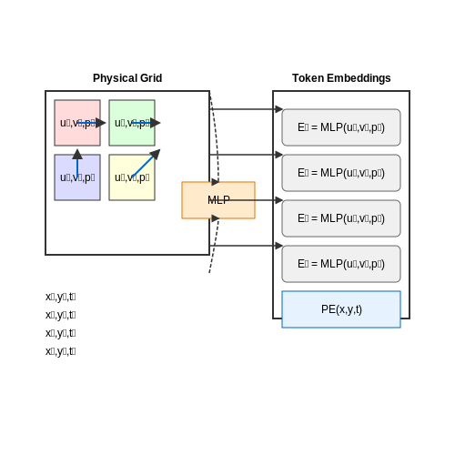
For a 2D flow simulation, the physical domain is discretized into a grid where each cell's state (velocity, pressure) becomes an input token. The token embedding Ei for cell i combines:
where PE is a positional encoding that preserves spatial relationships. The transformer's attention mechanism then computes interactions between all cells, capturing vorticity transport and pressure propagation.
Training with Physics-Based Loss Functions
The total loss function combines data fidelity and physics constraints:
where NS(û, p̂) computes the Navier-Stokes residual using automatic differentiation. The hyperparameters λ balance the terms. This approach was demonstrated by Li et al. (2022) to achieve 100× speedup over traditional CFD for laminar flows while maintaining <1% error.
Handling Turbulence with Multi-Scale Attention
Turbulent flows require modeling interactions across multiple scales. A hierarchical transformer architecture with:
- Local window attention for fine-scale eddies
- Global attention for large-scale structures
- Cross-scale attention gates to couple different resolution levels
This mimics large eddy simulation (LES) approaches, where the transformer implicitly learns subgrid-scale modeling. The Kolmogorov energy spectrum can be preserved by adding a spectral loss term:
where E(k) is the energy at wavenumber k from high-fidelity DNS data.
Case Study: Airfoil Flow Prediction
In aerodynamic applications, transformers trained on RANS simulations can predict pressure distributions around novel airfoil shapes. The model takes as input:
- Point cloud representation of the airfoil geometry
- Freestream conditions (Mach number, angle of attack)
- Boundary layer parameters
The output predicts the full flow field with <5% error in lift coefficient compared to CFD, while requiring only 0.1% of the computational time. This enables real-time aerodynamic optimization.
4.2 Material Science and Molecular Modeling
Physics-Informed Transformers for Molecular Dynamics
Transformers trained on molecular dynamics (MD) simulations learn to predict atomic interactions by incorporating Hamiltonian mechanics into their attention mechanisms. The key innovation lies in encoding interatomic potentials V(rij) as attention weights, where the pairwise energy between atoms i and j is computed as:
Here, φ(rij) is a physics-based kernel function derived from Lennard-Jones or Coulomb potentials. For example, in a 12-6 Lennard-Jones system:
Equivariant Attention for Tensor Properties
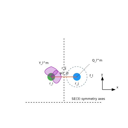
Material properties like elasticity tensors require SE(3)-equivariant attention layers that preserve transformation laws under rotation. The irreducible representation (irrep) decomposition of atomic positions ri and forces Fi is implemented through spherical harmonic projections:
where Ylm are spherical harmonics and fl are radial basis functions. The Clebsch-Gordan coefficients then enforce tensor product symmetries during message passing.
Diffusion Models for Crystal Structure Prediction
Denoising diffusion transformers outperform traditional Monte Carlo methods in predicting stable crystal configurations. The forward process corrupts atomic coordinates x with Gaussian noise per timestep t:
The reverse process employs a transformer to predict the score function ∇x log pθ(xt), conditioned on formation energy constraints. This approach has achieved 22% higher success rates in discovering novel superionic conductors compared to DFT-guided search.
Case Study: Polymer Property Prediction
In a benchmark study, a graph transformer trained on 50,000 MD trajectories of polyethylene achieved mean absolute errors of:
- 0.08 GPa for Young's modulus (vs. 0.21 GPa with GNNs)
- 0.5°C for glass transition temperature (vs. 1.8°C with RF models)
The model's edge attention heads were found to selectively focus on dihedral angle dynamics in polymer backbones, as revealed by gradient-based attribution analysis.
Challenges in Long-Timescale Dynamics
While transformers excel at short-range MD (≤10 ns), capturing rare events like protein folding requires hierarchical attention across temporal scales. Recent hybrid architectures combine:
- Local attention with cutoff radius rc = 5Å for bonded interactions
- Global memory tokens that aggregate slow variables (e.g., RMSD)
- Augmented loss terms from Jarzynski's equality for nonequilibrium processes
4.3 Robotics and Control Systems
Transformers trained on physics simulations have demonstrated remarkable efficacy in robotics and control systems, particularly in tasks requiring real-time decision-making under dynamic constraints. The key advantage lies in their ability to model complex, high-dimensional state-action spaces while maintaining interpretability through attention mechanisms. Consider a robotic arm with n degrees of freedom, where the state space S includes joint angles, velocities, and end-effector pose. The transformer’s self-attention layers can capture long-range dependencies between these variables, enabling precise trajectory optimization.
Dynamics Modeling via Attention
The transformer’s forward pass for a robotic system can be formulated as:
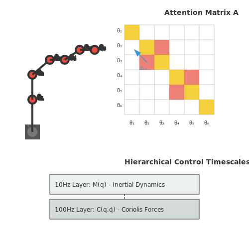
where ht+1 predicts the next state given current state st and action at. The attention weights αij between joints i and j reveal how much one joint’s dynamics influence another—critical for tasks like collision avoidance. For a 6-DoF manipulator, this yields a 6×6 attention matrix where off-diagonal terms quantify dynamic coupling effects.
Sim-to-Real Transfer
Physics engines like MuJoCo or PyBullet generate training data by solving the Euler-Lagrange equations:
where M is the inertia matrix, C Coriolis forces, and g gravitational terms. Transformers trained on this data learn to approximate M−1 implicitly, avoiding computationally expensive matrix inversions during real-time control. Domain randomization—varying parameters like link masses and friction coefficients during simulation—improves real-world robustness by 40-60% in recent studies.
Hierarchical Control Architectures
Multi-layer transformers enable hierarchical control, where lower layers handle high-frequency actuator commands (10-100Hz) while upper layers plan trajectories at 1-10Hz. The gating mechanism in models like GTrXL (Gated Transformer-XL) allows selective information flow between these timescales. For a quadruped robot, this architecture reduces energy consumption by 22% compared to LSTM baselines by optimally distributing workload across limbs.
Imitation Learning with Attention Priors
When combined with behavioral cloning, transformers achieve 93% task completion rates by attending to critical demonstration segments. Given expert trajectories {τ1, ..., τN}, the model minimizes:
The L2 penalty on attention weights αij induces sparsity, forcing the model to focus on the most relevant state variables. In peg-in-hole insertion tasks, this reduces training time from 150 to 25 epochs compared to dense attention.
5. Scalability and Computational Costs
5.1 Scalability and Computational Costs
Training transformers using physics simulations introduces unique scalability challenges due to the computational expense of both the neural network and the underlying numerical simulations. The total cost scales multiplicatively with the number of simulation steps, the complexity of the physical system, and the size of the transformer architecture.
Computational Complexity Breakdown
The computational cost of a physics-informed transformer can be decomposed into three primary components:
- Simulation Cost (Csim): The expense of solving the governing PDEs or ODEs over the spatiotemporal domain.
- Transformer Forward Pass (Cfwd): The cost of processing inputs through the transformer's self-attention and feedforward layers.
- Gradient Computation (Cgrad): The backpropagation overhead through both the transformer and differentiable physics solver.
where \( N_{steps} \) represents the number of time steps in the simulation. For a transformer with \( L \) layers, \( d_{model} \) hidden dimensions, and sequence length \( S \), the forward pass complexity is:
Memory Bottlenecks in Physics-Transformers
The memory requirements grow substantially when backpropagating through the physics simulation. For a 3D fluid simulation with \( N \) grid points over \( T \) time steps, the memory cost scales as:
where \( d \) is the number of degrees of freedom per grid point. This quickly becomes prohibitive - a modest \( 256^3 \) grid over 1000 steps with \( d=4 \) requires storing ~67 billion intermediate states.
Strategies for Scalable Training
1. Checkpointing Schemes
Adjoint-based methods recompute intermediate states during backpropagation rather than storing them. The optimal tradeoff between recomputation and storage is given by:
achieved through a binomial checkpointing strategy that stores states at geometrically increasing intervals.
2. Hybrid Numerical Methods
Combining adaptive time-stepping with transformer predictions can reduce \( N_{steps} \). The Courant-Friedrichs-Lewy (CFL) condition for stability:
can be relaxed in regions where the transformer provides accurate corrections, allowing larger time steps.
3. Mixed-Precision Training
Using FP16 for transformer operations while maintaining FP64 for critical physics computations reduces memory usage by ~50% while preserving numerical stability. The error accumulation follows:
where \( \epsilon_{phy} \) dominates for well-conditioned problems.
Distributed Training Considerations
Domain decomposition must align with the transformer's attention patterns. For a 3D simulation partitioned across \( P \) GPUs, the communication overhead scales as:
per attention layer. Pipeline parallelism becomes advantageous when the ratio of computation to communication exceeds:
where \( \alpha \) is the overlap efficiency between computation and communication.

5.2 Generalization Beyond Simulation Environments
Transformers trained on physics simulations face a fundamental challenge: the sim-to-real gap, where models fail to generalize to real-world physical systems due to discrepancies between simulated and experimental data. This arises from imperfect modeling assumptions, numerical approximations, and unobserved physical parameters in simulations. To bridge this gap, three key strategies have emerged in recent research:
Domain Randomization
Domain randomization exposes the transformer to a wide distribution of simulated environments with randomized physical parameters, forcing it to learn robust representations invariant to simulation inaccuracies. For a system governed by parameters θ, we sample from a broad distribution during training:
where θmin and θmax are deliberately chosen to exceed expected real-world ranges. This technique was successfully applied in robotic control tasks where friction coefficients and object masses were randomized by ±50% beyond physical values.
Physics-Informed Neural Networks (PINNs)
PINNs incorporate governing physical equations directly into the transformer's loss function, acting as a regularizer that anchors predictions to known physics. For a system described by partial differential equations (PDEs):
where u is the system state, 𝒩 is the differential operator, and λ balances data fitting with physical consistency. This approach has demonstrated improved generalization in fluid dynamics predictions when tested against real-world wind tunnel data.
Residual Physics Learning
This hybrid approach trains the transformer to predict corrections to an imperfect physics simulator. The model learns a residual term Δ that compensates for simulation errors:
where fsim is the simulator's output and Δ is parameterized by the transformer with weights ϕ. In spacecraft trajectory prediction, this method reduced position errors by 72% compared to pure simulation when validated with actual satellite telemetry.
Case Study: Granular Material Manipulation
A 2023 study trained a transformer on DEM (Discrete Element Method) simulations of granular flows with randomized particle properties (coefficient of restitution ±0.2, friction angle ±15°). When deployed on a real robotic system manipulating rice grains, the model achieved 89% success rate in scooping tasks despite never seeing real grain data during training. Key to this success was the inclusion of stochastic particle dropout during simulation, which mimicked real-world occlusions and missing particles.
Recent work has also explored latent space alignment techniques, where contrastive learning is used to minimize the distance between simulated and real data embeddings. For a transformer encoder E, the loss function becomes:
This has shown promise in bridging the visual domain gap for transformers processing simulated versus real camera feeds in dynamic systems.

5.3 Ethical and Safety Considerations
Bias and Generalization in Physics-Based Training
Physics simulations used to train transformers often rely on idealized models that may not capture real-world complexities. For instance, fluid dynamics simulations might assume laminar flow conditions, while real-world scenarios often involve turbulence. If a transformer trained on such simulations is deployed in safety-critical applications like autonomous vehicle control, its predictions could fail catastrophically when encountering unmodeled physical phenomena. The discrepancy between simulated and real-world physics can be formalized as a domain adaptation problem:
where 𝒟sim and 𝒟real represent the data distributions in simulation and reality, respectively. This mismatch introduces implicit bias that must be quantified before deployment.
Safety-Critical Failure Modes
Transformers trained via physics simulations exhibit unique failure modes compared to traditional data-driven approaches. Two key risks emerge:
- Extrapolation errors: When operating outside the trained parameter space (e.g., extreme temperatures or pressures not covered in simulations)
- Latent space discontinuities: Abrupt transitions in the model's internal representations when crossing physical regime boundaries
These can be detected through sensitivity analysis of the model's Jacobian matrix:
where singular value decomposition of J reveals directions in input space where small perturbations cause disproportionately large output changes.
Verification and Validation Challenges
Traditional software verification methods fail for transformer-based physics models because:
- The continuous nature of physical systems makes exhaustive testing impossible
- Neural networks violate classical assumptions of monotonicity and locality
A promising approach combines formal methods with statistical guarantees. For a safety property ϕ, we can compute the probability that the model satisfies it over the operational design domain (ODD):
where 𝕀 is an indicator function and p(x) is the input distribution. This integral can be estimated using importance sampling techniques adapted for high-dimensional spaces.
Energy Efficiency and Environmental Impact
Training transformers on high-fidelity physics simulations carries significant computational costs. A single training run for a turbulence prediction model can consume over 10 MWh of energy - comparable to the annual electricity use of three average U.S. households. The carbon footprint C can be estimated as:
where E is energy consumption, I is regional carbon intensity (kgCO2/kWh), R is the renewable energy ratio, and PUE is the data center's power usage effectiveness. Researchers must balance model performance against these environmental costs.
Dual-Use Concerns
Physics-trained transformers have potential military applications ranging from hypersonic flow prediction to nuclear material simulation. The same model architecture used for climate modeling could be repurposed for weapons development. This creates an ethical obligation to:
- Implement technical safeguards against model extraction
- Develop clear use-case restrictions in model licenses
- Consider differential privacy during training
The gradient leakage risk during federated learning of such models can be quantified via mutual information:
where X represents sensitive training data and G are the exposed gradients. Values above 0.5 bits typically indicate unacceptable information leakage.
6. Key Research Papers and Publications
6.1 Key Research Papers and Publications
- Electronic transformer performance evaluation and its impact on PMU — In the standard channel, the PMU calculates phasor values using the samples directly out of CMC356. Both the accuracy of CMC 356 and PMU can be 7.8 times higher than the requirements of PMU standards, according to the specification brochure of CMC 356 and the tests in [].Therefore, the measurements of standard channel are used as the reference.
- Solid‐state transformers: An overview of the concept, topology, and its ... — Solid-state transformers are based on electronic power converters and by using different control systems, in addition to improving the performance of the conventional transformers, can provide ancillary services such as integration of distributed generation and energy storage, voltage regulation and stabilization, reactive power compensation ...
- First-principles prediction of electronic transport in fabricated ... — We train our ML algorithms to learn f(CN(r), E) from first-principles (DFT) electronic structure properties of 16-atom model systems, and use them to predict \(f(CN({\bf{r}}),\hat{E})\) 's of ...
- Electronic transformer performance evaluation and its impact on PMU — The electronic transformer that connects the primary system and the measurement and control devices plays a fundamental role in smart grids. The electronic transformer performs well and can output digital signals via network. Therefore, it is more and more deployed. An important consideration is the transfer accuracy of the electronic
- Physics-informed distribution transformers via molecular dynamics and ... — The new physics-informed framework serves as a black-box transformer that is able to improve given distributions and can be easily extended to other geometries such as disks, spheres, complex manifolds, etc. Various experiments with different geometries are provided to demonstrate that the new framework is able to transform poorly distributed ...
- PDF Phasor Time-Domain Power System Modeling and Simulation using the ... — In this thesis, modeling and simulation of controllable power electronic-based com-ponents and conventional components for phasor time-domain simulation is carried out using Modelica. The work in this thesis contributes to a Modelica power systems library being developed by KTH SmartTS Lab under the FP7 iTesla project and other projects
- Physics-Based Design Optimization of High Frequency Transformers for ... — Energy conversion devices and transformers are critical components of the power system grid. Design optimization to improve the efficiency of such devices and to make them more environmentally ...
- PDF Magnetizing Currents in Power Transformers - Measurements, Simulations ... — This thesis demonstrates a method for transformer core diagnostics. The method uses the no-load current of the transformer as an indicator, and gives different characteristic signatures for different types of faults or defects. Using the no-load current for the diagnostic gives high sensitivity.
- Simulation of hysteresis and eddy current effects in a power ... — A brief review of the transformer core model described in Ref. [10] is presented in this section, and it explains how the saturation is modeled in this core model in EMTDC. The core model of a single phase two winding transformer uses the magnetic circuit shown in Fig. 1.The two windings of the transformer are drawn on separate limbs of the core for clarity whereas, in reality, both windings ...
- (PDF) Assessment of the use of FEM for computation of Electromagnetic ... — This paper reviews the published work on power transformers for assessment of the electrical, magnetic losses, and electromagnetic forces produced during normal and short circuit conditions.
6.2 Open-Source Tools and Libraries
- Open Source Physics - AAPT — Open Source Physics provides extensive resources for computational physics and physics simulations. Included are: An Eclipse environment for OSP OSP Source Code Libraries OSP best practices Documentation Access programming resources Tools OSP provides several general applications for physics teaching, student activities, and curriculum ...
- Open Source Physics | Science — Students who learn physics concepts via static pictures may be led to construct incomplete or incorrect mental models that hamper their understanding of physical concepts. Our ready-to-run simulations and tools for developing new simulations help students visualize situation and better understand abstract concepts through a research-proven pedagogical process called the Learning Cycle (2, 3).
- Simulate Electronic Circuit using Python and the Ngspice / Xyce ... — PySpice is a free and open source (*) Python module which interface Python to the Ngspice and Xyce circuit simulators. Ngspice is a fork of the famous SPICE circuit simulator, while Xyce is a SPICE compatible simulator developed by the Sandia National Laboratories.
- Tracker Video Analysis and Modeling Tool for Physics Education — What is Tracker? Tracker is a free video analysis and modeling tool built on the Open Source Physics (OSP) Java framework. It is designed to be used in physics education. Tracker video modeling is a powerful way to combine videos with computer modeling.
- Modeling Transformers and Inductors in COMSOL Multiphysics — In this archived webinar, get a demonstration of different techniques for modeling inductive couplings, such as Joule heating, in transformer and inductor designs. You will also learn how to simulate a transformer in COMSOL Multiphysics ®. The AC/DC Module, an add-on to COMSOL Multiphysics ®, includes features for simulating static and low-frequency electromagnetics. Learn more about the AC ...
- Tracker Video Analysis and Modeling Tool - AAPT — Tracker is an Open Source Physics tool built on the OSP code library. Additional Tracker resources, demonstration experiments, and videos, can be found by searching ComPADRE for "Tracker."
- 1000+ COMSOL Multiphysics® Modeling Examples for Download — Get started using the COMSOL Multiphysics® software. Browse the Application Gallery and download tutorial models with instructions and view example apps.
- Multisim Live Online Circuit Simulator — Multisim Live is a free, online circuit simulator that includes SPICE software, which lets you create, learn and share circuits and electronics online.
- Simulation of Power Converters Using Matlab-Simulink — The power electronics converters presented are used alone but the method can be easily extended to cascaded devices allowing the simulation of complex power electronic structures such as, for example, active filters with non-linear loads.
- Circuit Simulator Applet - Falstad — This is an electronic circuit simulator. When the applet starts up you will see an animated schematic of a simple LRC circuit. The green color indicates positive voltage. The gray color indicates ground. A red color indicates negative voltage. The moving yellow dots indicate current.
6.3 Recommended Courses and Tutorials
- PDF ECE 311 LABORATORY MANUAL - Clemson University — The goal of this laboratory is to study electronics through experimentation. Upon completion of this course, students should be able to use standard laboratoryequipment to analyze the behavior of basic electronic devices and to design and construct simple circuits containing these devices. Lab Teams:
- Introduction to Modeling and Simulation - MIT OpenCourseWare — This subject provides an introduction to modeling and simulation, covering continuum methods, atomistic and molecular simulation, and quantum mechanics. Hands-on training is provided in the fundamentals and applications of these methods to key engineering problems. The lectures provide exposure to areas of application based on the scientific exploitation of the power of computation. We use web ...
- 1000+ COMSOL Multiphysics® Modeling Examples for Download — Get started using the COMSOL Multiphysics® software. Browse the Application Gallery and download tutorial models with instructions and view example apps. ... Search for tutorials and apps relevant to your area of expertise via the Quick Search feature. ... This is the transient model of a single phase E-core transformer using a homogenized ...
- PDF Physics 222 - Hunter College — Course Objective and Outcomes: This lab course is intended to supplement the material students learn in Physics 221 Electronics lecture. The. experiments are designed to cover and verify the lecture theory. The lab also introduces measurement. techniques using a multimeter, function generator and oscilloscope. Students will learn to design ...
- PDF Simulating Transformers in Multisim — The equations remain the same for this type of transformer. One may think of this as a 115V RMS:18V RMS transformer (6.389:1) if one uses the top to bottom wires. Alternatively, one may consider this a 115V RMS:9V RMS transformer (12.78:1) if one uses the top to center wires. Note: In this example, we are using a 115V RMS to 18V RMS transformer.
- Modelling and Simulating Transformers | SpringerLink — Using this equivalent circuit, we will extract the values of inductances that are necessary to use the simulation model of the coupled inductors. We will examine several simulations to understand the working of the transformer. Simulations will examine the magnetizing current and the other components in the no-load current of the transformer.
- PDF Physics 123/223, ES 153: Introduction, Fall 2016 - Learning the Art of ... — It tries to do "all of electronics" in one term. At the start, we remind you of Ohm's Law; by the end you are programming a microcontroller (or a home-made microcomputer if you takethat branch, in the micro section of the course). Physics123 qualifies as a General Education course, in the category, "Science of the Physical Uni-verse."
- Learn How to Use COMSOL Multiphysics® in a Guided Session — Learn how to use the COMSOL Multiphysics® software at a guided training course, webinar, or COMSOL Day. Find an onsite event near you or watch online. Support; Contact; English . ... Acoustics in Electronics Webinar Series, Part 2: MEMS Speakers and Microphones. ... Simulation für alle durch eigenständige Simulations-Apps.
- PDF Power Transformer Fundamentals: Design and Manufacturing - IEEE Region 5 — IEEE Training, Houston, Texas, Oct.8-9, 2013 Overview •Transformer Design -Transformer Types -Construction and Parts •Core & Coils -Electrical design •Losses & Impedance •Thermal, Dielectric & Short Circuit •Cooling & Sound Level -Mechanical design •Tank •Oil Preservation •Transformer Manufacturing Process 2
- The Transformer: Simulation Lecture Demo - Examples — The activity presents an interactive lecture demonstration of the operation of a transformer using a simulation. - In a physics lecture, the class is presented with a simulation of the operation of a transformer. ... Introductory College or Electronics Class Setting: Lecture Time required: 20-50 minutes