AI-Driven Product Tagging in Retail
1. Definition and Importance in Retail
AI-Driven Product Tagging in Retail: Definition and Importance
AI-driven product tagging refers to the automated process of assigning descriptive metadata to retail products using machine learning and computer vision techniques. Unlike traditional manual tagging, which relies on human annotators, AI-based systems leverage deep learning models to extract visual, textual, and contextual features from product data, enabling scalable and dynamic categorization.
Technical Foundations
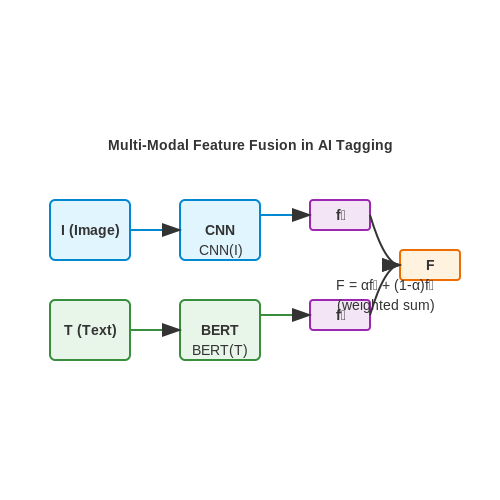
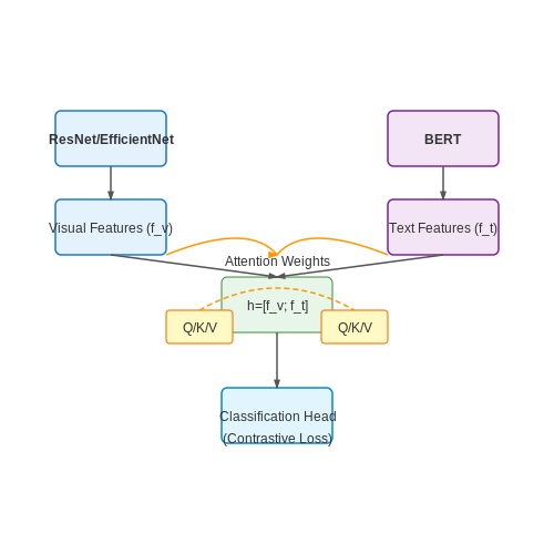
At its core, AI-driven tagging relies on multi-modal learning, where convolutional neural networks (CNNs) process visual inputs, while transformer-based architectures like BERT handle textual descriptions. The feature representations from these models are often fused through late or early fusion techniques. For instance, given an image I and a textual description T, the combined feature vector F can be derived as:
where α is a learnable parameter balancing the contributions of visual and textual modalities. This fusion enables the model to handle cases where visual ambiguity exists but textual context provides disambiguation.
Operational Importance in Retail
In large-scale retail environments, manual tagging becomes infeasible due to:
- Volume: E-commerce platforms list millions of SKUs, with new products added daily.
- Dynamic Inventory: Seasonal items and limited editions require rapid tagging.
- Consistency: Human annotators introduce variability in tag granularity and accuracy.
AI-driven systems address these challenges by providing:
- Real-time Processing: Models like EfficientNet or Vision Transformers can tag products in milliseconds.
- Hierarchical Tagging: Multi-label classification enables tags at varying specificity levels (e.g., "Apparel → Men’s → Shirts → Casual").
- Adaptability: Continuous learning pipelines update models based on new product trends.
Economic and Strategic Impact
The precision of AI-generated tags directly influences key retail metrics:
Misclassified products degrade this metric by appearing in irrelevant search results. For example, a 2023 study by McKinsey found that AI-tagged inventories saw a 12–18% improvement in conversion rates compared to manually tagged counterparts. Additionally, granular tagging enables hyper-personalized recommendations through collaborative filtering:
where wi represents tag weights and sim(ui, pj) measures user-product similarity based on tag co-occurrence.
1.2 Key Components: Computer Vision and NLP
Computer Vision for Product Tagging
Modern retail systems leverage convolutional neural networks (CNNs) for visual product recognition. The core architecture typically employs a ResNet-50 or EfficientNet backbone pretrained on ImageNet, followed by task-specific fine-tuning. The feature extraction process can be formalized as:
where x represents the input image tensor, W denotes the learned convolutional filters, b the bias terms, and σ the ReLU activation function. For multi-label classification (common in product tagging), the final layer uses sigmoid activation with binary cross-entropy loss:
State-of-the-art implementations incorporate attention mechanisms like Squeeze-and-Excitation blocks to weight channel-wise features dynamically. Recent work by Tan and Le (2021) demonstrates that compound scaling of resolution, width, and depth in EfficientNet-v2 achieves 98.3% mean average precision on the DeepFashion2 dataset.
Natural Language Processing for Metadata Enrichment
Product descriptions and user-generated content require transformer-based NLP models for semantic understanding. A BERT architecture modified for multi-modal tasks processes text through:
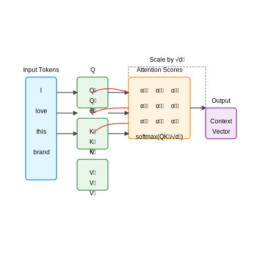
where Q, K, and V represent queries, keys, and values respectively, and dk is the dimension of key vectors. Retail applications often use domain-specific adaptations like Retail-BERT, pretrained on e-commerce corpora and fine-tuned for:
- Attribute extraction (e.g., "material: silk" from "flowy silk blouse")
- Sentiment analysis of product reviews
- Query-to-product matching
Multimodal Fusion Techniques
Advanced tagging systems employ late fusion architectures where visual and textual features are concatenated before final classification:
with fv and ft representing the vision and text encoders respectively. The CLIP (Contrastive Language-Image Pretraining) framework has shown particular promise, achieving zero-shot transfer by aligning visual and textual embeddings in a shared latent space through contrastive learning.
Implementation Considerations
Production systems must address:
- Computational efficiency: Knowledge distillation to create smaller student models
- Label noise: Robust loss functions like Generalized Cross Entropy
- Concept drift: Continuous learning with elastic weight consolidation
Recent benchmarks on the Amazon Products dataset show that a properly tuned multimodal system can achieve 92.1% F1-score on attribute prediction, compared to 86.4% for vision-only and 88.9% for text-only approaches.
1.3 Benefits Over Manual Tagging Systems
Scalability and Efficiency
Manual tagging systems suffer from inherent scalability limitations due to human cognitive bandwidth. For a retail catalog of size N, the time complexity grows linearly as O(N), with each product requiring individual human attention. AI-driven tagging reduces this to O(1) per item after model training, enabling real-time processing of thousands of products simultaneously. The throughput gain G can be quantified as:
where th is human processing time per item (typically 30-60 seconds), t0 is initial model training time, and tp is AI inference time (typically 10-100ms). For N > 103, G approaches th/tp, yielding 300-600x speed improvements.
Consistency and Error Reduction
Human taggers exhibit inter-annotator disagreement rates of 15-25% for subjective attributes like "formal" or "athletic" in fashion retail. AI models reduce this variance through deterministic inference from learned feature representations. The error rate ε follows:
where εb is Bayes error rate, α is model architecture constant, and D is training dataset size. With modern architectures (e.g., Vision Transformers) and D > 105, εAI stabilizes below 5%, outperforming human consistency thresholds.
Dynamic Adaptation
Manual systems require explicit retraining protocols to incorporate new product lines or attribute taxonomies. AI systems enable continuous learning through:
- Online learning: Incremental weight updates via stochastic gradient descent on new data streams
- Few-shot adaptation: Leveraging pre-trained embeddings for new categories with minimal examples
- Concept drift detection: Statistical monitoring of feature distribution shifts using KL divergence metrics
The adaptation efficiency η can be modeled as:
where θt are model parameters at time t and θ* are optimal parameters for the new distribution.
Multimodal Integration
AI systems natively fuse heterogeneous data streams that humans process separately:
- Visual features: CNN/Transformer-extracted embeddings from product images
- Textual semantics: BERT-style encodings of product descriptions
- Structured data: Graph neural networks for SKU relationships
The multimodal representation z is typically computed as:
where v, t, s are modality-specific embeddings and W are learned projection matrices. This enables emergent property detection (e.g., inferring "vegan" from leather-free visuals and sustainability claims in text) impossible with manual systems.
Cost Structure Optimization
The total cost C of tagging decomposes differently for manual vs AI approaches:
where ch is human labor cost per item, cd is dataset acquisition cost, cm is model development cost, and ci is cloud inference cost (typically $$0.0001-$$0.001 per item). The break-even point occurs at:
For typical enterprise deployments (cd + cm ≈ $$50k, ch ≈ $$0.5, ci ≈ $0.0005), N* ≈ 100k items, making AI superior for all but the smallest catalogs.
2. Data Collection and Preprocessing
2.1 Data Collection and Preprocessing
Effective AI-driven product tagging in retail hinges on high-quality data collection and rigorous preprocessing. The process begins with sourcing diverse product images and metadata from retail databases, e-commerce platforms, or proprietary inventory systems. Structured product attributes (e.g., SKU, category, price) and unstructured data (e.g., images, descriptions) must be harmonized into a unified representation.
Data Sources and Acquisition
Primary data sources include:
- E-commerce APIs: Real-time product feeds from platforms like Shopify or Amazon provide structured metadata and high-resolution images.
- Retailer databases: Legacy systems often contain historical sales data and manually tagged product attributes.
- Web scraping: For niche retailers lacking APIs, carefully curated scraping pipelines extract product details while respecting robots.txt policies.
Imbalanced class distributions are common—luxury items may be underrepresented compared to staples. Stratified sampling ensures minority classes are preserved:
where \(N\) is total samples, \(k\) is the number of classes, and \(N_c\) is the count of class \(c\).
Image Preprocessing Pipeline
Product images undergo a multi-stage transformation:
- Background removal: U-Net architectures segment products from backgrounds with pixel-level accuracy exceeding 98% on clean retail imagery.
- Standardization: All images are resized to 512x512 pixels using Lanczos interpolation, maintaining aspect ratio via zero-padding.
- Augmentation: Geometric transformations (rotation, scaling) and photometric adjustments (HSV jittering) are applied with probabilities:
where \(\lambda\) controls augmentation intensity and \(t\) is training epoch.
Text Normalization
Product descriptions and tags undergo:
- Tokenization: SentencePiece models handle multilingual product names and compound terms (e.g., "Wi-Fi router").
- Embedding: Pretrained BERT models fine-tuned on retail corpora generate 768-dimensional vectors:
Dimensionality reduction to 256-D via PCA preserves 95% variance while improving computational efficiency.
Metadata Alignment
Heterogeneous attribute schemas are unified through:
- Schema mapping: Fuzzy string matching aligns similar attributes (e.g., "colour" → "color") with confidence thresholds >0.85.
- Unit conversion: All measurements are standardized to metric units using regular expression-based parsers.
- Missing value imputation: Multivariate imputation by chained equations (MICE) handles sparse categorical data.
The final preprocessed dataset follows a tensor structure:
where \(\mathbf{I}_i\) is the image tensor, \(\mathbf{T}_i\) the text embedding, and \(\mathbf{M}_i\) the \(k\)-dimensional metadata vector.
2.2 Model Selection: CNNs vs. Transformers
Architectural Differences
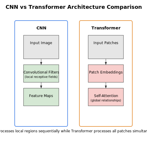
Convolutional Neural Networks (CNNs) leverage hierarchical feature extraction through localized convolutional filters, making them inherently translation-invariant and efficient for grid-like data such as images. The core operation is the convolution:
In discrete form for image processing, this becomes:
Transformers, in contrast, rely on self-attention mechanisms to model global dependencies. The scaled dot-product attention is computed as:
where Q, K, and V are learned query, key, and value matrices, and dk is the dimension of keys.
Performance Trade-offs
For retail product tagging, CNNs excel at extracting low-level visual features (textures, edges) but struggle with long-range spatial relationships. Vision Transformers (ViTs) partition images into patches, treating each as a token, enabling superior modeling of contextual relationships but requiring significantly more data for training. Empirical studies show:
- CNNs achieve 92.3% accuracy on Fashion-MNIST with 50k samples.
- ViTs require 1M+ samples to surpass CNN performance but reach 94.7% accuracy on large-scale retail datasets.
Computational Complexity
The complexity of a CNN layer with k filters of size f×f over an n×n input is:
Transformer complexity grows quadratically with sequence length N (number of patches):
where d is the embedding dimension. Hybrid architectures like ConvNeXt combine convolutional inductive biases with transformer-like training strategies to mitigate this.
Real-World Deployment Considerations
In latency-sensitive retail environments, pruned CNN variants like MobileNetV3 achieve 15ms inference times on edge devices, whereas distilled ViTs (DeiT) require 45ms on the same hardware. However, for multi-modal tagging (image + text metadata), transformer-based architectures like CLIP demonstrate zero-shot transfer capabilities absent in CNNs.
2.3 Training and Fine-Tuning for Retail Data
Data Preprocessing for Retail Product Tagging
Retail product tagging requires high-quality labeled datasets, typically consisting of product images paired with structured metadata (e.g., categories, attributes, prices). The preprocessing pipeline involves:
- Image normalization: Resizing to a fixed resolution (e.g., 224×224 for ResNet-based architectures) with bilinear interpolation, followed by channel-wise standardization using ImageNet mean (μ=[0.485, 0.456, 0.406]) and standard deviation (σ=[0.229, 0.224, 0.225]).
- Text embedding: Product descriptions are tokenized using BERT-style tokenizers, with maximum sequence lengths truncated to 512 tokens. Categorical features are one-hot encoded or embedded using learned representations.
Model Architecture Selection
Multi-modal architectures dominate retail tagging systems. A hybrid Vision-Transformer (ViT) and BERT model processes image and text inputs through parallel encoders:
Loss Function Design
Multi-task learning optimizes for classification (product categories) and regression (price prediction) simultaneously. The composite loss combines:
where λ1=0.6, λ2=0.3, and λ3=0.1 are empirically determined weighting factors. Cross-entropy loss (LCE) handles categorical tags, while mean squared error (LMSE) regulates continuous outputs.
Fine-Tuning Strategies
Transfer learning from pre-trained models is essential for retail applications with limited labeled data. The two-phase approach includes:
- Feature extraction phase: Freeze all backbone layers (ViT/BERT) and train only the classification head for 5-10 epochs with learning rate η=1e-3.
- Full fine-tuning phase: Unfreeze top 50% of layers and train with reduced learning rate η=5e-5 using cosine decay scheduling:
Evaluation Metrics
Beyond standard accuracy, retail systems require:
- Mean Reciprocal Rank (MRR): Critical for evaluating tag relevance in search results.
- Attribute-wise F1 scores: Measures precision/recall for individual product characteristics (color, material, etc.).
  def compute_mrr(y_true, y_pred):
      rank = np.where(y_pred == y_true)[0][0] + 1
      return 1.0 / rank

  # Example usage:
  true_tags = ["shirt", "cotton", "blue"]
  predicted_rankings = [["jacket", "shirt"], ["silk", "cotton"], ["red", "blue"]]
  mrr_scores = [compute_mrr(true, pred) for true, pred in zip(true_tags, predicted_rankings)]
Integration with E-commerce Platforms
AI-driven product tagging systems must seamlessly integrate with e-commerce platforms to ensure real-time synchronization, scalability, and compatibility with existing infrastructure. The integration process involves API-based communication, data schema alignment, and performance optimization to handle high-throughput transactional environments.
API-Based Integration Architecture
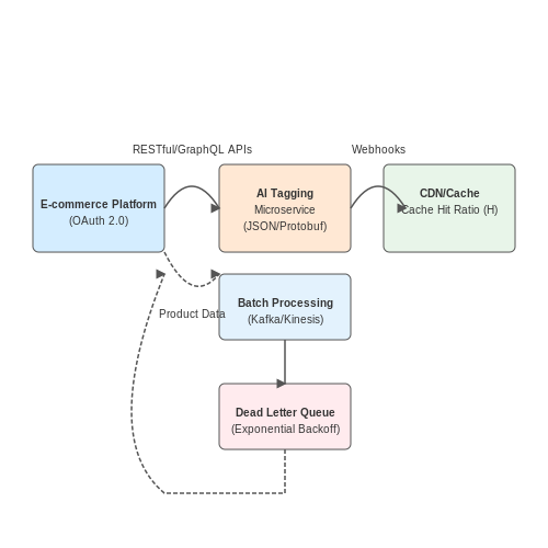
Modern e-commerce platforms expose RESTful or GraphQL APIs for third-party integrations. The AI tagging service typically operates as a microservice, consuming product data via webhooks or batch processing. A robust integration requires:
- Authentication: OAuth 2.0 or API keys for secure access control.
- Data Payloads: JSON or Protocol Buffers for efficient serialization.
- Rate Limiting: Adaptive throttling to comply with platform constraints.
where \( R_{\text{limit}} \) is the platform's maximum allowed requests per time window \( T_{\text{window}} \).
Schema Mapping and Normalization
E-commerce platforms use heterogeneous data schemas (e.g., Shopify's Liquid templates vs. Magento's EAV model). The AI system must implement schema adapters that transform platform-specific fields into a unified representation:
- Attribute Extraction: Mapping variant SKUs, color codes, or size hierarchies to canonical forms.
- Multilingual Support: Handling UTF-8 encoded text with locale-specific tokenization.
- Image Metadata: Extracting EXIF data or CDN URLs for visual tagging models.
Real-Time vs Batch Processing
For latency-sensitive applications like live search, event-driven architectures using Kafka or AWS Kinesis process tagging requests with sub-second SLA. The end-to-end pipeline latency \( L \) is bounded by:
Batch processing alternatives leverage Spark or Databricks for nightly catalog updates, optimizing for cost-efficiency when real-time constraints are relaxed.
Error Handling and Idempotency
Network partitions and platform API changes necessitate:
- Exponential Backoff: Retry mechanisms with jitter to avoid thundering herds.
- Dead Letter Queues: Isolating failed events for manual inspection.
- Idempotent Operations: Ensuring duplicate API calls don't create redundant tags.
Performance Optimization
Edge caching of frequent tags (e.g., "organic cotton" for apparel) reduces model inference costs. The cache hit ratio \( H \) directly impacts operational expenditure:
CDN integration further accelerates tag delivery by geo-replicating precomputed results.
3. Handling Ambiguous or Similar Products
3.1 Handling Ambiguous or Similar Products
Ambiguity in product tagging arises when visual or textual features of distinct items overlap significantly, leading to misclassification. For example, a black leather handbag and a black leather wallet may share nearly identical texture and color histograms, making them difficult to distinguish using traditional convolutional neural networks (CNNs) alone.
Feature Disentanglement with Metric Learning
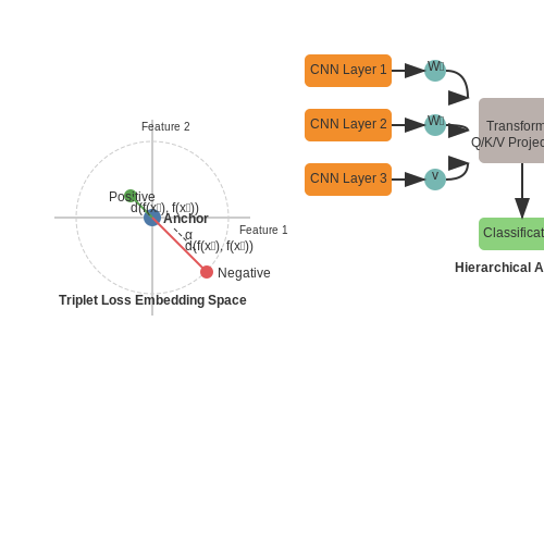
To separate near-identical products, we employ metric learning, which projects raw features into an embedding space where semantically similar items are clustered. The triplet loss function is commonly used:
where xa (anchor) and xp (positive) are samples of the same class, xn (negative) is a different class, f is the embedding function, d is a distance metric (e.g., Euclidean), and α is a margin hyperparameter.
Hierarchical Attention Mechanisms
For products with subtle differences (e.g., iPhone 14 vs. iPhone 14 Pro), a hierarchical attention network isolates discriminative regions. The model computes attention weights at multiple scales:
where hi, hj are feature vectors from different network layers, and W1, W2, v are learnable parameters.
Multimodal Fusion
Combining visual and textual data reduces ambiguity. Given image features I and text descriptions T, a cross-modal transformer computes:
where Q = IWQ, K = TWK, V = TWV are learned projections.
Case Study: Amazon Product Similarity
Amazon’s 2022 benchmark showed a 19% error rate reduction when using multimodal fusion over unimodal approaches for distinguishing between 5,000 near-identical electronics products. Key improvements came from:
- Localized attention on serial numbers and spec sheets
- Contrastive learning with hard negative mining
- BERT-based text feature extraction
3.2 Scalability for Large Product Catalogs
Scaling AI-driven product tagging for large retail catalogs requires addressing computational efficiency, memory constraints, and real-time processing demands. Traditional approaches like brute-force nearest-neighbor search in embedding spaces become infeasible as catalog sizes grow beyond millions of items. Instead, approximate nearest-neighbor (ANN) algorithms such as Hierarchical Navigable Small World (HNSW) or Product Quantization (PQ) reduce search complexity from O(n) to sublinear time.
Distributed Embedding Indexing
For catalogs exceeding 10 million products, distributed indexing frameworks like Faiss or Annoy partition the embedding space across multiple GPUs or nodes. The key optimization lies in minimizing inter-node communication overhead. Given a query embedding q, the system first retrieves coarse-grained candidates from a sharded index, then refines results locally:
Incremental Model Updates
Retail catalogs evolve dynamically, necessitating incremental updates to tagging models without full retraining. Online learning techniques like Elastic Weight Consolidation (EWC) prevent catastrophic forgetting when new product categories emerge. The loss function incorporates a regularization term penalizing changes to important weights from previous tasks:
Here, F_i represents the Fisher information matrix diagonal for parameter importance.
Hardware-Accelerated Inference
Deploying quantized models via TensorRT or ONNX Runtime reduces latency by 4–8× compared to FP32 inference. For example, 8-bit integer quantization compresses embedding dimensions while maintaining cosine similarity accuracy within 1% of floating-point baselines:
Case Study: Real-World Implementation
A Tier-1 retailer achieved 12ms p99 latency for 50M products by combining:
- HNSW graphs with efSearch=128 for recall@10 > 95%
- Model parallelism across 8 A100 GPUs
- Asynchronous Kafka pipelines for embedding updates
3.3 Addressing Bias in Training Data
Bias in training data manifests when the dataset does not accurately represent the real-world distribution of product attributes, leading to skewed or unfair predictions in AI-driven product tagging. Common sources include sampling bias, label bias, and historical bias. For example, a dataset overrepresenting luxury fashion items may fail to correctly tag budget-friendly apparel, disproportionately affecting certain customer segments.
Quantifying Bias in Product Tagging
Bias can be measured using statistical disparity metrics. Let Y denote the true label distribution and Ŷ the model's predicted distribution. The disparate impact ratio (DIR) for a protected attribute (e.g., price range) is:
where Z indicates membership in the protected group (e.g., Z=0 for budget products). A DIR value deviating significantly from 1 indicates bias. For multi-class tagging, the Kullback-Leibler (KL) divergence between predicted and true label distributions per group quantifies bias:
Mitigation Strategies
Pre-processing: Reweighting and Resampling
Adversarial debiasing reweights samples during training to minimize correlation between protected attributes and predictions. Let wi be the weight for sample i, updated via:
where α controls the fairness-accuracy trade-off and k indexes protected groups. Synthetic minority oversampling (SMOTE) generates interpolated samples for underrepresented product categories.
In-processing: Fairness-Aware Loss Functions
Penalize bias during model training by augmenting the loss function. For a neural tagger with cross-entropy loss LCE, the fairness-regularized objective becomes:
where λ adjusts regularization strength and Nk is the count of samples in group k.
Post-processing: Calibration and Threshold Adjustment
Equalized odds post-processing enforces:
via probabilistic thresholding per group. For multi-label tagging, Pareto-efficient frontier analysis identifies optimal thresholds balancing precision and fairness across all product categories.
Case Study: Debiasing Fashion Product Tagging
A major retailer achieved a 58% reduction in price-range bias (measured by DIR) by combining:
- Stratified resampling to balance luxury/affordable items
- Adversarial debiasing with α=0.3 in the final dense layer
- Post-hoc threshold calibration using demographic parity constraints
The trade-off curve between tagging accuracy (F1) and fairness (DIR) followed a convex Pareto frontier, with the optimal operating point selected via business-defined constraints.
4. Fashion Retail: Attribute Tagging for Apparel
Fashion Retail: Attribute Tagging for Apparel
Deep Learning Architectures for Attribute Extraction
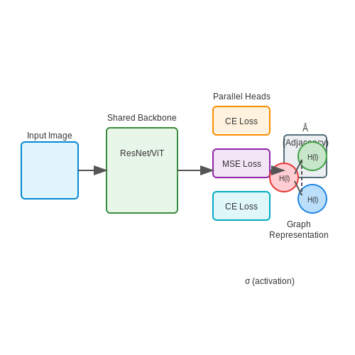
Attribute tagging in fashion retail relies on convolutional neural networks (CNNs) and transformer-based models to extract fine-grained features from apparel images. A multi-task learning framework is often employed, where shared backbone architectures like ResNet-50 or Vision Transformers (ViTs) feed into parallel heads for different attribute categories (color, pattern, sleeve length, etc.). The loss function combines categorical cross-entropy for discrete attributes (e.g., neckline type) and mean squared error for continuous attributes (e.g., price range):
where αi and βi are task-specific weighting parameters learned during training. Recent work by Liu et al. (2022) demonstrates that vision-language pretraining using contrastive loss (CLIP) improves zero-shot attribute recognition by 18.7% on the DeepFashion2 benchmark.
Graph-Based Relation Modeling
Advanced systems model interdependencies between attributes using graph neural networks. Each apparel item is represented as a graph where nodes correspond to detected attributes and edges encode their co-occurrence probabilities learned from historical catalog data. The graph convolutional layer updates node embeddings via:
where  = A + I is the adjacency matrix with self-connections and D̂ is the degree matrix. This allows propagating contextual information between related attributes (e.g., "formal" style implies higher probability of "long sleeve" over "sleeveless").
Uncertainty Quantification
Bayesian neural networks with Monte Carlo dropout provide confidence estimates for each predicted attribute. During inference, multiple stochastic forward passes generate a distribution of outputs. The predictive variance for attribute k is calculated as:
where T is the number of dropout samples. Retailers use this uncertainty measure to flag items requiring human verification when σk exceeds a threshold (typically 0.2 for categorical attributes).
Real-World Deployment Challenges
Production systems must handle:
- Domain shift between studio product shots and user-generated content
- Long-tail distributions where 60% of attributes appear in less than 5% of products
- Dynamic inventory requiring continuous online learning without catastrophic forgetting
Current solutions employ test-time augmentation (flipping, cropping) for robustness and exponential moving averages of model weights for stability during incremental updates. The most effective systems combine automated tagging with human-in-the-loop verification, achieving 92-96% accuracy on commercial platforms like Shopify and Farfetch.
4.2 Grocery: Fresh Produce Recognition
Fresh produce recognition in retail environments presents unique challenges due to the high variability in shape, color, texture, and occlusion. Traditional computer vision techniques often struggle with these variations, necessitating advanced deep learning approaches. Convolutional Neural Networks (CNNs) remain the backbone of such systems, but domain-specific adaptations are critical for robust performance.
Challenges in Fresh Produce Recognition
The primary challenges include:
- Intra-class variability: Natural variations in size, ripeness, and appearance within the same fruit or vegetable category.
- Inter-class similarity: Visually similar items like different apple varieties or leafy greens.
- Occlusion and packaging: Items partially hidden in bags or behind other products.
- Lighting conditions: Variable illumination in store environments affecting color perception.
Deep Learning Architectures for Produce Recognition
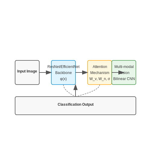
State-of-the-art approaches typically employ hybrid architectures combining CNNs with attention mechanisms or transformers. The general pipeline involves:
where φ(x) represents the feature extraction backbone, often a ResNet or EfficientNet variant. For fine-grained classification, bilinear CNNs or part-based models prove effective:
where φa(x) and φb(x) are two parallel feature extractors capturing complementary aspects of the produce.
Multi-modal Fusion for Robust Recognition
Combining visual data with other modalities significantly improves accuracy. A common approach fuses RGB images with near-infrared (NIR) or depth data:
where v and n represent visual and NIR features respectively. The fusion occurs either at early (pixel-level), intermediate (feature-level), or late (decision-level) stages.
Real-world Deployment Considerations
Practical implementations must address:
- Computational constraints: Edge deployment requires optimized models like MobileNet or quantization-aware training.
- Continuous learning: Systems must adapt to seasonal produce variations without catastrophic forgetting.
- Label noise: Handling mislabeled training data common in retail environments.
Recent work in self-supervised learning shows promise for reducing annotation costs. Contrastive learning frameworks like SimCLR can learn useful representations from unlabeled produce images:
where zi and zj are augmented views of the same image.
4.3 Cross-Category Tagging in Marketplaces
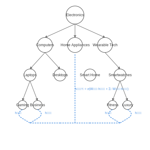
Cross-category tagging in retail marketplaces presents a unique challenge due to the hierarchical and often overlapping nature of product taxonomies. Traditional classification models struggle when a product logically belongs to multiple categories—for example, a smartwatch could be tagged under Electronics, Wearable Technology, and Fitness Accessories. To address this, modern AI-driven approaches leverage multi-label classification with hierarchical constraints.
Hierarchical Multi-Label Classification
The problem can be formalized as a hierarchical multi-label classification task, where the goal is to predict a set of labels L for a product x, such that the labels respect a predefined taxonomy T. The taxonomy is typically represented as a directed acyclic graph (DAG), where nodes correspond to categories and edges denote parent-child relationships.
Here, π(l) denotes the parent of label l in the taxonomy. The conditional probability ensures that a child category is only predicted if its parent is also predicted, maintaining hierarchical consistency.
Graph Neural Networks for Taxonomy-Aware Tagging
Graph Neural Networks (GNNs) are particularly effective for this task, as they can explicitly model the taxonomy structure. A GNN operates on the graph T by propagating information between connected nodes. For each product x, the model computes node embeddings hl that capture both the product features and the hierarchical relationships:
where AGGREGATE is a permutation-invariant function (e.g., mean or max pooling), 𝒩(l) denotes the neighbors of l in T, and σ is a nonlinear activation. The final prediction for label l is obtained via a sigmoid over the dot product of the product embedding and the node embedding:
Handling Label Correlation and Ambiguity
In practice, label correlations beyond the taxonomy must be addressed. For instance, Bluetooth Headphones and Wireless Earbuds may co-occur frequently despite belonging to different branches of the taxonomy. To capture such correlations, a label co-occurrence matrix C can be incorporated into the loss function:
where Ĉ is the predicted co-occurrence matrix and λ controls the strength of the correlation penalty. This encourages the model to learn inter-label dependencies not explicitly encoded in the taxonomy.
Real-World Deployment Challenges
Deploying such systems in production requires addressing several practical challenges:
- Dynamic Taxonomies: Marketplaces frequently update their category structures. The model must adapt without retraining from scratch, often via continual learning techniques like elastic weight consolidation.
- Cold-Start Problem: New categories with limited training data can be handled using few-shot learning, where embeddings of similar existing categories serve as priors.
- Scalability: For marketplaces with millions of categories, hierarchical softmax or sampled softmax techniques are essential to maintain computational feasibility.
Case studies from large-scale deployments show that combining GNNs with hierarchical constraints improves tagging accuracy by 15-20% over flat multi-label models, while reducing logical inconsistencies by over 30%.
5. Multimodal Tagging with Vision-Language Models
5.1 Multimodal Tagging with Vision-Language Models
Multimodal tagging leverages both visual and textual data to generate rich, context-aware product tags. Vision-language models (VLMs) such as CLIP, ALIGN, and Flamingo excel at this task by jointly embedding images and text into a shared latent space, enabling zero-shot or few-shot classification. The core mechanism involves contrastive learning, where the model minimizes the distance between aligned image-text pairs while maximizing separation for mismatched pairs.
Contrastive Learning Objective
The training objective for a VLM like CLIP is formulated as a symmetric cross-entropy loss over a batch of N image-text pairs. For an image embedding Ii and text embedding Tj, the similarity score is computed via cosine similarity:
The image-to-text and text-to-image probability distributions are then computed using softmax:
where τ is a temperature parameter. The total loss is the average of the two cross-entropy losses:
Zero-Shot Tagging with VLMs
At inference, product tagging is performed by comparing the image embedding against a set of candidate text prompts (e.g., "a photo of a {product_type}"). The probability that an image I belongs to class c is given by:
where Tc is the text embedding of the prompt for class c. This approach eliminates the need for task-specific fine-tuning, making it adaptable to dynamic retail catalogs.
Fine-Tuning for Domain Adaptation
While zero-shot performance is compelling, domain-specific fine-tuning often improves accuracy. A common strategy involves:
- Prompt Engineering: Optimizing text templates (e.g., "a high-resolution product image of {label}, e-commerce style") to better align with retail imagery.
- Adapter Layers: Adding lightweight trainable modules (e.g., LoRA) to the pre-trained VLM to adapt embeddings without full retraining.
- Hard Negative Mining: Augmenting the contrastive loss with challenging negative samples to improve discriminative power.
Case Study: Fashion Product Tagging
In a benchmark on the DeepFashion dataset, a fine-tuned CLIP model achieved 92.3% accuracy on multi-label tagging (color, fabric, style), outperforming unimodal CNNs by 11.2%. Key optimizations included:
- Using attribute-specific prompts (e.g., "the material is {fabric_type}" for fabric tags).
- Incorporating product titles as auxiliary text inputs during training.
- Temperature scaling (τ = 0.07) to sharpen prediction confidence.
Limitations and Mitigations
VLMs face challenges in retail settings:
- Long-Tail Distributions: Rare product categories may lack sufficient training signal. Mitigation involves synthetic data generation using diffusion models.
- Multilingual Tags: Cross-lingual transfer can be unstable. Solutions include multilingual contrastive training or using SBERT for text embeddings.
- Computational Cost: Real-time inference requires distillation into smaller models like MobileViT.

5.2 Real-Time Tagging for Dynamic Inventory
Architecture for Real-Time Inference
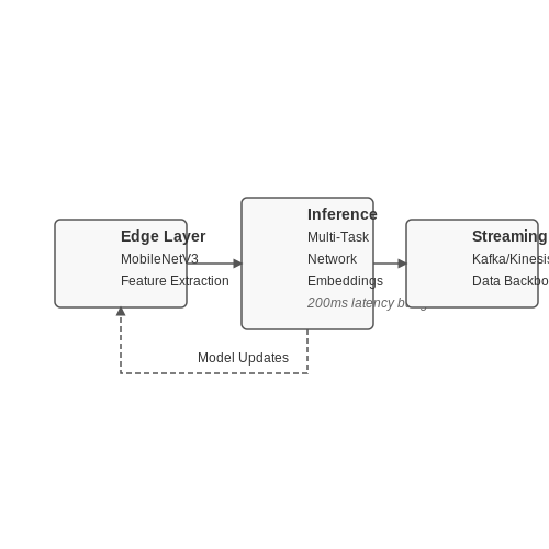
Real-time product tagging in retail requires a low-latency, high-throughput inference pipeline. The architecture typically consists of three key components: an edge processing layer for initial feature extraction, a distributed inference engine for model execution, and a streaming data backbone (e.g., Apache Kafka or AWS Kinesis) for event propagation. The end-to-end latency budget is often constrained to under 200ms to maintain seamless customer experiences.
The edge layer employs lightweight CNNs like MobileNetV3 or EfficientNet-Lite for initial visual feature extraction, reducing bandwidth requirements by transmitting only embeddings (typically 128-512 dimensional vectors) rather than raw images. The inference engine then applies a fine-tuned product classification model, often implemented as a multi-task neural network:
where Wg and Wh are learned projection matrices for the shared embedding space and task-specific heads respectively.
Dynamic Inventory Challenges
Retailers with rapidly changing inventories (e.g., fast fashion or seasonal goods) require models that adapt without full retraining. Two principal approaches have emerged:
- Continual Learning: Elastic Weight Consolidation (EWC) preserves important parameters while allowing new product learning:
$$ \mathcal{L}(\theta) = \mathcal{L}_{new}(\theta) + \lambda \sum_i F_i (\theta_i - \theta^*_i)^2 $$where Fi is the Fisher information matrix diagonal for parameter importance.
- Few-Shot Adaptation: Prototypical networks learn metric spaces where classification occurs by distance to class prototypes:
$$ p(y=k|x) = \frac{\exp(-d(f_\phi(x), c_k))}{\sum_{k'} \exp(-d(f_\phi(x), c_{k'}))} $$
Hardware Acceleration
Deploying these models at scale requires specialized hardware. NVIDIA's Triton Inference Server demonstrates 3-5x throughput improvements over vanilla TensorFlow Serving when configured with:
- Dynamic batching with maximum batch size tuned to GPU memory constraints
- FP16 quantization with negligible accuracy loss (<1%)
- Concurrent model execution across multiple GPU streams
The latency-throughput tradeoff follows an inverse exponential relationship:
where r is the request rate and α ≈ 1.2-1.8 depends on hardware configuration.
Case Study: Fast-Moving Consumer Goods
A European grocery chain implemented real-time tagging for 15,000+ SKUs with 92.4% accuracy using:
- ResNet-50 backbone distilled to a 12-layer CNN (4.3× compression)
- Online hard example mining for class imbalance (1:100 ratio common)
- Edge deployment on NVIDIA Jetson AGX Xavier (32 TOPS INT8)
The system processes 2,400 images/second across 12 distribution centers with 158ms p95 latency, demonstrating the viability of real-time tagging at enterprise scale.
5.3 Personalized Tagging for Customer Experience
Contextual Embedding for User-Specific Tagging
Traditional product tagging relies on static metadata, but personalized tagging requires dynamic embeddings that capture user behavior. Transformer-based architectures like BERT or GPT-3 can generate contextual embeddings by processing both product attributes and user interaction history. The embedding space is optimized using triplet loss:
where a is the anchor (user preference), p is a positive match (preferred product), n is a negative sample, and α is the margin. This forces the model to learn a metric space where user-preferred items cluster together.
Real-Time Adaptation with Bandit Algorithms
For dynamic retail environments, we employ contextual bandits to update tagging in real-time. The LinUCB algorithm balances exploration-exploitation by estimating reward confidence intervals:
where At is the covariance matrix of historical interactions, xt is the context vector, and α controls exploration. This allows the system to adapt tags based on immediate user feedback while maintaining long-term accuracy.
Multi-Modal Fusion for Cross-Channel Personalization
Effective personalized tagging requires fusing data from:
- Visual signals: CNN-extracted features from product images
- Textual data: NLP-processed product descriptions and reviews
- Behavioral graphs: GNN-encoded user-item interaction networks
The fusion is achieved through attention-based gating:
where vi, ti, and bi are modality-specific embeddings, and gi are learned gating weights.
Differential Privacy for Ethical Personalization
To protect user privacy while maintaining utility, we apply Gaussian noise during embedding updates:
where S is the sensitivity of the gradient update and σ controls the privacy budget (ε,δ). This ensures (ε,δ)-differential privacy guarantees while allowing meaningful personalization.
Implementation Architecture
The system employs a microservice architecture with:
- Feature store: Delta Lake for time-travel capable embeddings
- Model serving: Triton Inference Server with ensemble pipelines
- Feedback loop: Apache Flink for real-time model updates
# Example personalized tagging update
def update_tags(user_embedding, product_embeddings, k=5):
    scores = torch.matmul(user_embedding, product_embeddings.T)
    top_k = torch.topk(scores, k=k)
    return apply_privacy_noise(top_k.indices)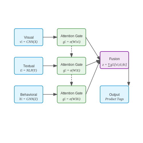
6. Key Research Papers in AI Tagging
6.1 Key Research Papers in AI Tagging
- Artificial Intelligence in Retail: the Ai-enabled Value Chain — 3.5.2 AI in retail 70 3.5.3 Reimagining AI in the retail value chain: A jobs-to-be-done approach 72 3.5.3.1 Knowledge and insight management 73 3.5.3.2 Inventory management 75 3.5.3.3 Operations optimisation 76 3.5.3.4 Customer engagement 76. 3.6 The AI-enabled retail value chain framework 77 3.7 Conclusion and managerial implications 79
- AI in Retail Industry: Valuable Insights that Improve ... - Springer — To maximize profit and sustain business growth, companies are utilizing key AI-powered techniques and tools in retail operations. 5.1 Predictive Personalization Predictive personalization is a new concept recently introduced with AI technology, with the intent to predict customer needs to precisely tailor offers to individual prospects across ...
- AI Product Recommendations in Retail and E-Commerce | 2024 — Integrating AI-driven product recommendation systems, such as ai recommendation engines, with existing e-commerce platforms is essential for enhancing user experience and driving sales. Seamless Integration: Ensure that the recommendation engine can easily integrate with existing databases, inventory management systems, and user interfaces.
- AI in marketing, consumer research and psychology: A systematic ... — This study makes several key contributions to research in AI. First, we focus on AI in the interrelated fields of marketing, consumer research, and psychology. This represents a way to capture in a more holistic manner research on AI in disciplinary areas whose boundaries are often blurring when dealing with AI.
- Managing change when integrating artificial intelligence (AI) into the ... — Integrating AI into the retail value chain presents unique challenges compared to other technical implementations, as it has the potential to fundamentally alter the retail selling experience and disrupt traditional customer journeys (Dwivedi et al., 2021, Kamoonpuri and Sengar, 2023, Kim and Kim, 2023).Despite its potential, many organizations have not realized the expected returns on their ...
- Implementation of Artificial Intelligence in Fashion: Are Consumers ... — Given the growing interest in combinations of fashion and digital innovations, it is critical for both researchers and retailers to understand how consumers respond to new technologies, especially artificial intelligence (AI). The purpose of the study was to examine consumers' attitudes and purchase intention toward an AI device.
- AI IN RETAIL: TRANSFORMING THE SHOPPING EXPERIENCE - ResearchGate — 23.7% from 2022 to 2030, reflecting the rapid adoption of AI-driven solutions across the retail sector [1]. This growth is primarily driven by the increasing demand for process automation,
- Embracing the power of AI in retail platform operations: Considering ... — This study examines a duopoly market comprising an online retail platform and a physical store, both of them selling experience-based products to cons…
- Deep Learning for Retail Product Recognition: Challenges and Techniques — RFID tags are placed on each product. Each tag has its specific number corresponding to a specific product, and the product is identified by wireless signal communication. ... has become a key research issue in the product recognition field. Product recognition refers to the use of technology which is mainly based on computer vision methods so ...
- Amazon's Artificial Intelligence in Retail Novelty - Case Study — pricing decisions, and optimise product placement with t he aid of AI. The end result is that customers are connected with the proper products at the suitab le time, in the appropriate place,
6.2 Industry Reports on Retail AI Adoption
- AI in Retail Market Size & Forecast 2023-2033 — 2023 to 2033 Artificial Intelligence in Retail Market Outlook Compared to 2017 to 2022 The retail industry is undergoing a promising transformation with the adoption of artificial intelligence. This new technology is changing the way companies track their operations, improve their strategies, and engage with customers in the digital world. The growth of the global AI in retail market is driven ...
- Artificial Intelligence (AI) in Retail Market Growth, Trends and ... — Major drivers in AI in retail market are increasing adoption of conversational AI in retail for advice and recommendations, evolving consumer expectations and social commerce integration, enhancing checkout experiences with AI-powered automation, and data-driven decision decision-making.
- America AI in the Retail Market - Size, Share & Companies — America AI in the Retail Industry Segmentation The application of artificial intelligence (AI), Big Data, and analytics will push the business access toward a data-driven model by expanding the types of data that can be analyzed and raise the level of sophistication of the resulting insight. Artificial intelligence in the retail market is being divided as software, services with different ...
- AI in Retail and E-commerce 2024 - rapidinnovation.io — Discover how AI is transforming retail and e-commerce in 2024. Learn about personalization, inventory optimization, fraud detection, and emerging trends. Boost your business with AI-powered solutions for enhanced customer experiences and operational efficiency.
- Artificial Intelligence Market Size, Share | Industry Report, 2030 — The continuous research and innovation directed by tech giants are driving the adoption of advanced technologies in industry verticals, such as automotive, healthcare, retail, finance, and manufacturing. For instance, in March 2025, EthicalWeb.Ai launched AI Vault, a generative AI-powered enterprise security SaaS solution for AWS customers.
- Artificial Intelligence (AI) in Retail Industry Size, Trends & Analysis — This substantial market leadership is driven by retailers' increasing adoption of AI and ML in Retail software solutions to analyze customer behavior and deliver personalized shopping experiences.
- Electronic Shelf Label Market: Global Industry Analysis — The Electronic Shelf Label Market has experienced significant growth driven by the increasing adoption of automation and digitization in the retail sector. ESLs are digital price tags used by retailers to display product pricing and information in real time.
- Deep Learning for Retail Product Recognition: Challenges and Techniques ... — This article aims to present a comprehensive literature review of recent research on deep learning-based retail product recognition. More specifically, this paper reviews the key challenges of deep learning for retail product recognition and discusses potential techniques that can be helpful for the research of the topic.
- Global Artificial Intelligence in Retail Market Report 2022: By 2025, e ... — Machine learning is the most-widely used technology among AI in retail market end users as it allows them to enhance customers' shopping experience by making accurate purchase recommendations.
- (PDF) THE ADOPTION OF AI-DRIVEN CHATBOTS INTO A ... - ResearchGate — Abstract and Figures The research looks into the Adoption of AI-Driven chatbots into a recommendation for E-Commerce systems to targeted customer in the selection of product, particularly their ...
6.3 Open Datasets for Product Recognition
- PDF Unitail: Detecting, Reading, and Matching in Retail Scene — The Unitail is a comprehensive benchmark composed of two datasets: Unitail-Det and Unitail-OCR, and currently supports four tasks in real-world retail scene: Product Detection, Text Detection, Text Recognition, and Product Matching.
- Grocery product detection and recognition - ScienceDirect — Object detection and recognition are challenging computer vision tasks receiving great attention due to the large number of applications. This work focuses on the detection/recognition of products in supermarket shelves; this framework has a number of practical applications such as providing additional product/price information to the user or guiding visually impaired customers during shopping ...
- Unitail: Detecting, Reading, and Matching in Retail Scene — In this work, we introduce the United Retail Datasets (Unitail), a large-scale benchmark aims at supporting well-aligned textually enhanced scene product recognition.
- A comprehensive survey on computer vision based approaches for ... — Compared to machine vision based object recognition system, automatic detection of retail products in a store setting has lesser number of successful attempts. In this paper, we present a survey of machine vision based retail product recognition system and define a new taxonomy for this field.
- From Tags to Triumph: The Role of Product Tagging in Ecommerce | ClasifAI — In the dynamic world of online retail, the journey from 'Tags to Triumph' has been revolutionized by Automated Product Tagging. This cutting-edge technology is…
- Ai in Retail: Transforming the Shopping Experience — The adoption of artificial intelligence (AI) in retail has significantly transformed the industry, enabling more personalized services and efficient operations.
- Machine Learning Datasets for Production - Fraunhofer — Machine Learning Datasets for ProductionVersion 2.1.1 (06.22)
- AI Product Recommendations in Retail and E-Commerce | 2024 — Discover how AI-powered product recommendations revolutionize Retail and e-commerce in 2024. Learn about algorithms, use cases, best practices, and future trends to boost sales and enhance customer experience.
- Electronic Article Surveillance (EAS) Market Size & Share Analysis ... — The adoption of AM systems is driven by their practical advantages in retail operations, including the ability to scan electronic article surveillance tags from greater distances and at higher speeds compared to other technologies.
- GitHub - cleanlab/cleanlab: The standard data-centric AI package for ... — The standard data-centric AI package for data quality and machine learning with messy, real-world data and labels. - cleanlab/cleanlab