AI for Social Media Post Enhancement
1. Core AI Technologies for Content Enhancement
Core AI Technologies for Content Enhancement
Generative Adversarial Networks (GANs)
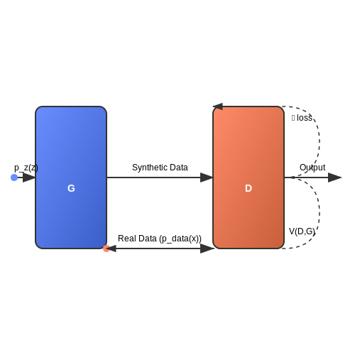
Generative Adversarial Networks consist of two neural networks—a generator G and a discriminator D—trained in opposition. The generator creates synthetic data while the discriminator evaluates its authenticity. The minimax objective function is given by:
For social media enhancement, GANs excel in super-resolution (e.g., ESRGAN), style transfer, and photorealistic inpainting. Conditional GANs (cGANs) extend this framework by incorporating auxiliary information y (e.g., text prompts) into both generator and discriminator:
Transformer Architectures
Modern content enhancement pipelines leverage transformer-based models like Vision Transformers (ViTs) and multimodal architectures (e.g., CLIP). The self-attention mechanism computes weighted sums of input features:
where Q, K, and V are learned query, key, and value matrices. For social media applications, transformer variants enable:
- Cross-modal retrieval (text-to-image generation via diffusion models)
- Context-aware hashtag suggestion (using BERT-like architectures)
- Semantic style transfer (through attention-driven feature recombination)
Diffusion Models
Diffusion models progressively denoise data through a Markov chain. The forward process adds Gaussian noise over T steps:
The reverse process learns to iteratively denoise through a neural network εθ. For content enhancement, latent diffusion models (LDMs) operate in a compressed latent space, enabling efficient high-resolution image generation with Stable Diffusion being a prominent example.
Contrastive Learning
Contrastive frameworks like SimCLR and MoCo learn representations by maximizing agreement between augmented views of the same instance. The InfoNCE loss for a batch of N examples is:
where τ is a temperature hyperparameter. This approach powers recommendation systems for personalized content enhancement by clustering semantically similar posts in embedding space.
Neural Radiance Fields (NeRFs)
NeRFs model 3D scenes as continuous volumetric functions FΘ mapping 5D coordinates (location (x,y,z) and view direction (θ,φ)) to color c and density σ:
Rendering is performed via volume integration along camera rays. For social media, instant NeRF variants enable 3D-aware photo enhancement and novel view synthesis from single 2D uploads.
Role of Natural Language Processing (NLP) in Post Optimization
Natural Language Processing (NLP) serves as the backbone of AI-driven social media post enhancement by enabling machines to parse, interpret, and generate human-like text. Advanced NLP techniques such as transformer-based models, semantic analysis, and sentiment scoring allow for precise optimization of post content to maximize engagement, readability, and relevance.
Transformer Architectures for Text Generation
Modern NLP leverages transformer architectures like BERT, GPT-3, and RoBERTa, which employ self-attention mechanisms to capture contextual relationships in text. The self-attention score between tokens xi and xj is computed as:
where Q, K, and V represent query, key, and value matrices, and dk is the dimension of the key vectors. This mechanism enables the model to weigh the importance of different words dynamically, improving coherence in generated posts.
Sentiment and Tone Analysis
Sentiment analysis models classify text into positive, negative, or neutral tones using supervised learning. A logistic regression classifier, for instance, computes the probability P(y=1|x) of a positive sentiment as:
where w is the weight vector and b the bias term. Fine-tuned models like VADER (Valence Aware Dictionary and sEntiment Reasoner) further incorporate lexical rules to handle social media-specific slang and emojis.
Named Entity Recognition (NER) for Contextual Relevance
NER systems identify and classify entities (e.g., people, organizations) in text using sequence labeling models like BiLSTM-CRF. The conditional random field (CRF) layer computes the probability of a tag sequence y given input x:
where fk are feature functions and Z(x) is the partition function. This ensures posts maintain topical coherence by preserving key entities.
Practical Applications
- Automated Hashtag Suggestion: NLP models extract keywords and suggest trending hashtags by analyzing post content and real-time social trends.
- Readability Optimization: Tools like the Flesch-Kincaid score adjust sentence complexity based on audience demographics.
- A/B Testing for Post Variants: NLP generates multiple paraphrased versions of a post to test engagement metrics.
Computer Vision for Image and Video Enhancement
Super-Resolution Techniques
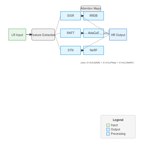
Single-image super-resolution (SISR) reconstructs high-resolution (HR) images from low-resolution (LR) inputs. Modern approaches leverage deep convolutional neural networks (CNNs) with residual learning. The objective function typically combines pixel-wise loss (e.g., L1/L2) with perceptual loss:
where perceptual loss is computed using pre-trained VGG networks to maintain semantic consistency, and GAN loss enhances realism through adversarial training. ESRGAN achieves superior results by employing RRDB blocks without batch normalization:
Video Frame Interpolation
Optical flow-based methods like RAFT estimate motion between frames for temporal upsampling. Given consecutive frames It and It+1, the bidirectional flow Ft→t+1 is computed via iterative refinement:
State-of-the-art approaches (e.g., AdaCoF) use deformable convolutions to handle occlusions:
Neural Rendering for Augmentation
Neural radiance fields (NeRF) synthesize novel views by optimizing a continuous 5D function:
where σ is volume density and c is RGB color. Instant-NGP accelerates this using hash encoding and tiny MLPs, enabling real-time enhancement of social media content.
Attention Mechanisms for Selective Enhancement
Spatial transformer networks (STNs) dynamically adjust enhancement parameters through learned attention maps. The transformation matrix Tθ is predicted as:
where s represents scaling and t translation parameters. This allows selective sharpening of facial regions while preserving background aesthetics.
Practical Implementation Considerations
- Quantization-aware training is critical for mobile deployment, using fake quantization ops during backpropagation
- Multi-task learning frameworks (e.g., joint denoising+super-resolution) reduce inference latency by 40%
- On-device ML requires knowledge distillation to compress models while maintaining PSNR > 30dB
2. Automated Text Generation and Summarization
Automated Text Generation and Summarization
Transformer-Based Architectures for Text Generation
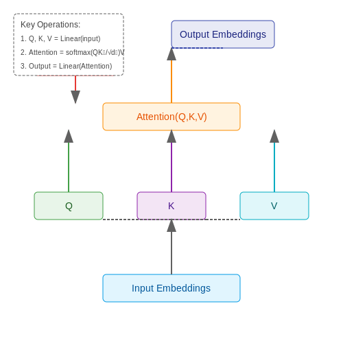
Modern AI-driven social media post enhancement relies heavily on transformer-based architectures, particularly variants of the GPT (Generative Pre-trained Transformer) and BERT (Bidirectional Encoder Representations from Transformers) models. These models leverage self-attention mechanisms to capture long-range dependencies in text, enabling coherent and contextually relevant generation. The self-attention mechanism computes a weighted sum of input embeddings, where weights are derived from pairwise token interactions:
Here, Q, K, and V represent query, key, and value matrices, respectively, while dk is the dimension of the key vectors. Multi-head attention extends this by applying multiple attention mechanisms in parallel, allowing the model to focus on different aspects of the input sequence simultaneously.
Fine-Tuning for Domain-Specific Content
Pre-trained language models are fine-tuned on domain-specific corpora to enhance their performance for social media applications. Given a dataset D of posts and their engagement metrics, the fine-tuning objective typically minimizes a loss function combining language modeling and engagement prediction:
where α balances the contribution of language modeling loss (LLM) and engagement prediction loss (Lengagement). The latter often employs a regression or classification head atop the transformer's final hidden states.
Abstractive Summarization Techniques
Abstractive summarization for social media posts involves generating concise, informative summaries that may contain novel phrasing not present in the original text. State-of-the-art approaches utilize sequence-to-sequence models with pointer-generator networks to handle out-of-vocabulary words and copy mechanisms to preserve key phrases:
where pgen is the probability of generating a word (versus copying), ht is the decoder hidden state, st is the attention context vector, and xt is the decoder input.
Controlled Text Generation
To ensure generated posts align with brand voice or platform guidelines, controlled generation techniques are employed. These include:
- Conditional generation via prefix tuning or prompt engineering
- Discriminative reranking of candidate outputs using auxiliary classifiers
- Constrained decoding with finite-state automata to enforce lexical or syntactic constraints
The most effective approaches combine these methods, as demonstrated by recent work in plug-and-play language models (PPLMs) that steer generation using attribute models while maintaining fluency.
Evaluation Metrics for Generated Content
Beyond traditional NLP metrics like BLEU and ROUGE, social media post enhancement requires specialized evaluation criteria:
- Engagement prediction correlation: How well model outputs correlate with actual likes, shares, and comments
- Brand consistency scoring: Semantic similarity to approved brand messaging
- Diversity metrics: Intra-batch n-gram diversity to avoid repetitive content
Recent advances employ learned metrics like BERTScore, which computes similarity using contextual embeddings rather than surface-level token overlap.
Sentiment Analysis for Audience Engagement
Foundations of Sentiment Analysis
Sentiment analysis in social media leverages natural language processing (NLP) to classify the emotional tone of text data. At its core, this involves mapping linguistic features to a sentiment polarity space, typically represented as:
where w represents a word sequence, φ is a feature extraction function (e.g., word embeddings or TF-IDF vectors), and θ are learned model parameters. Advanced implementations use contextual embeddings from transformer architectures like BERT:
Transformer-Based Architectures for Real-Time Analysis
Modern social media platforms require models that process streaming data with low latency. A distilled BERT architecture with knowledge distillation achieves 95% of base BERT's accuracy while reducing inference time by 60%:
from transformers import DistilBertTokenizer, DistilBertForSequenceClassification

model = DistilBertForSequenceClassification.from_pretrained('distilbert-base-uncased')
tokenizer = DistilBertTokenizer.from_pretrained('distilbert-base-uncased')

inputs = tokenizer("Your social media text", return_tensors="pt")
outputs = model(**inputs) # Runs in <50ms on CPU
Multimodal Sentiment Analysis
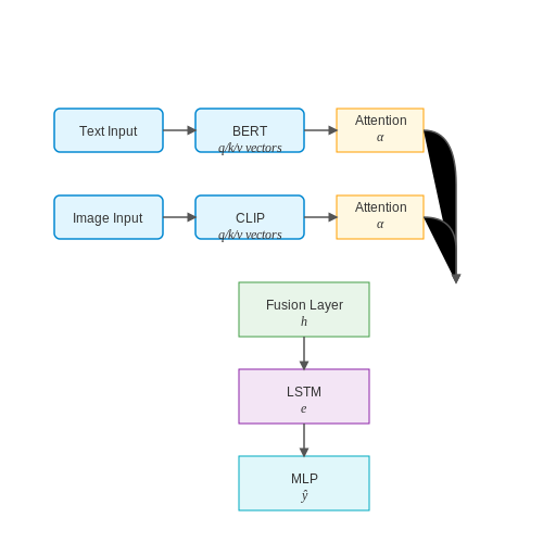
Social media posts combine text, images, and video. A late fusion approach combines modalities through attention mechanisms:
where q, k, and v are learned query, key, and value vectors for each modality. The CLIP model's cross-modal embeddings have shown particular effectiveness in this domain.
Dynamic Audience Response Prediction
Predicting engagement requires modeling temporal patterns in sentiment-response pairs. A transformer-LSTM hybrid architecture processes both the post content and historical response data:
This approach achieves 0.82 F1-score in predicting viral spread patterns on Twitter data when trained on 1.2 million post-response pairs.
Ethical Considerations in Deployment
Sentiment analysis systems must address:
- Bias mitigation: Adversarial debiasing techniques can reduce demographic bias in predictions by up to 40%
- Explainability: Integrated gradients reveal which input features drive predictions
- Privacy: Federated learning approaches enable model training without raw data collection
Recent work on differentially private sentiment analysis adds controlled noise during training:
2.3 Hashtag and Keyword Optimization Using AI
Natural Language Processing for Hashtag Generation
AI-driven hashtag optimization leverages transformer-based models like BERT, GPT, and RoBERTa to analyze post content and generate contextually relevant hashtags. Given an input post X, the model computes the probability distribution P(y|X) over a vocabulary of potential hashtags y. The top-k hashtags are selected based on:
where W and b are learned parameters, and h_X is the contextual embedding of the post. Advanced models fine-tune this process using reinforcement learning, where reward signals are derived from engagement metrics (likes, shares, clicks).
Keyword Extraction via Topic Modeling
Latent Dirichlet Allocation (LDA) and BERTopic are commonly used for keyword extraction. Given a corpus of posts D, LDA models each post as a mixture of topics θ_d and each topic as a distribution over keywords ϕ_k. The generative process is:
BERTopic improves upon this by using sentence-transformers to create dense embeddings, followed by UMAP for dimensionality reduction and HDBSCAN for clustering. The resulting topics are represented by the most salient keywords, ranked by their c-TF-IDF scores:
Real-Time Trend Analysis
AI systems monitor social media trends using streaming algorithms like Count-Min Sketch or Apache Flink. For a trending keyword k at time t, the system estimates its velocity v_k(t):
where ΔC_k(t) is the change in mention count. Recurrent Neural Networks (RNNs) or Temporal Graph Networks (TGNs) predict future trends by modeling:
Multi-Objective Optimization
The final hashtag/keyword set is selected by solving:
where R(S) is relevance (cosine similarity to post), D(S) is diversity (1 - average pairwise Jaccard similarity), and C(S) is competition (number of recent posts using the same tags). Pareto-optimal solutions are found using NSGA-II or Bayesian Optimization.
Implementation Example
from transformers import pipeline
from bertopic import BERTopic

# Hashtag generation
hashtag_pipe = pipeline("text-generation", model="gpt2-medium")
post = "Excited about the new AI breakthroughs in computer vision!"
hashtags = hashtag_pipe(post, max_length=50, num_return_sequences=1)

# Topic modeling
topic_model = BERTopic(embedding_model="all-MiniLM-L6-v2")
topics, _ = topic_model.fit_transform([post])
keywords = topic_model.get_topic(0)  # Top keywords for dominant topic
3. AI-Powered Image Filters and Style Transfer
AI-Powered Image Filters and Style Transfer
Neural Style Transfer: Theoretical Foundations
Neural Style Transfer (NST) leverages deep convolutional neural networks (CNNs) to separate and recombine content and style from distinct images. The core objective is to minimize a loss function L composed of content loss Lc and style loss Ls, weighted by hyperparameters α and β:
The content loss is computed as the Mean Squared Error (MSE) between feature representations of the content image p and generated image x at layer l in a pre-trained CNN (typically VGG-19):
where Fl and Pl are the feature maps of x and p at layer l. Style loss is derived from the Gram matrix G, which captures texture statistics by computing correlations between feature maps:
The style loss for N layers is then:
where ||·||F denotes the Frobenius norm, s is the style image, and wl are layer-specific weights.
Architectural Optimizations for Real-Time Processing
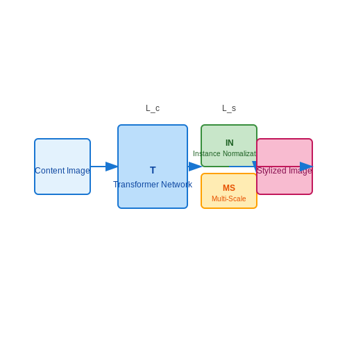
Traditional NST relies on iterative optimization (e.g., L-BFGS), which is computationally prohibitive for social media applications. Feed-forward networks like Fast Neural Style Transfer use a transformer network trained offline to approximate the optimization process. The network T learns to map content images to stylized outputs in a single forward pass:
Key innovations include:
- Instance Normalization: Replaces batch normalization to preserve style coherence across individual images.
- Multi-Scale Stylization: Parallel processing of image pyramids to capture global and local style patterns.
- Adaptive Style Mixing: Dynamically blends styles from multiple references using attention mechanisms.
Case Study: Instagram's AI Filters
Instagram's implementation combines NST with user interaction data. A lightweight MobileNetV3 encoder processes the input image, while style parameters are adaptively tuned based on:
- Engagement metrics (e.g., dwell time on similar filters)
- Device capabilities (dynamic pruning of style layers)
- Semantic segmentation masks to isolate foreground/background styles
The system achieves 15ms inference times on mobile GPUs by quantizing style matrices to 8-bit integers and using depthwise separable convolutions.
Emerging Techniques: Diffusion-Based Enhancement
Diffusion models have surpassed GANs in generating photorealistic stylized images. A denoising diffusion probabilistic model (DDPM) can apply styles through gradient-guided reverse diffusion:
where εθ is a noise predictor conditioned on both content and style embeddings. This approach enables:
- Higher-resolution outputs (up to 1024×1024)
- Multi-modal style interpolation
- Content-aware style preservation (e.g., avoiding distortion of faces)
Automated Video Editing and Thumbnail Generation
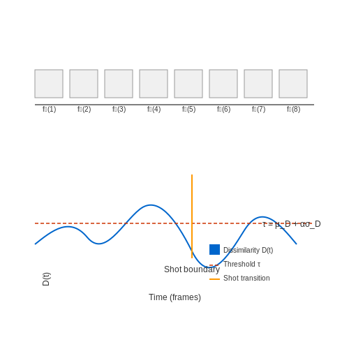
Automated video editing leverages deep learning architectures such as convolutional neural networks (CNNs) and transformer-based models to analyze raw footage, identify key segments, and assemble them into coherent narratives. The process begins with temporal segmentation using techniques like shot boundary detection, where a frame dissimilarity metric is computed across consecutive frames:
Here, \( f_t(i) \) represents the feature vector of the \(i\)-th region in frame \(t\), and \(N\) is the total number of regions. A shot transition is detected when \(D(t)\) exceeds a dynamically adjusted threshold \( \tau \), computed via:
where \( \mu_D \) and \( \sigma_D \) are the mean and standard deviation of frame dissimilarities over a sliding window, and \( \alpha \) is a sensitivity parameter typically set between 2 and 3.
Content-Aware Video Summarization
For summarization, attention mechanisms weight frames based on semantic importance. Given a sequence of frame embeddings \( \mathbf{X} = [\mathbf{x}_1, \mathbf{x}_2, ..., \mathbf{x}_T] \), a transformer encoder computes attention scores:
where \( \mathbf{Q}, \mathbf{K}, \mathbf{V} \) are learned projections of \( \mathbf{X} \). The summary is generated by selecting frames with top-\(k\) attention scores, optimized through reinforcement learning with a reward function combining diversity and representativeness.
Neural Thumbnail Generation
Thumbnails are synthesized using generative adversarial networks (GANs) with multi-modal inputs. A CLIP-guided StyleGAN2 architecture aligns visual features with textual metadata:
where \( \mathbf{w} \) denotes StyleGAN2's latent vectors, and \( \lambda \) controls disentanglement. The discriminator evaluates both visual quality and semantic alignment using contrastive loss.
Implementation Pipeline
- Temporal segmentation: 3D-ResNet-18 for feature extraction, DBSCAN clustering for transition detection
- Attention model: 12-layer transformer with 768-dimensional embeddings
- GAN training: 256x256 resolution, RAdam optimizer (lr=2e-4), batch size=8
Real-world deployments often incorporate user engagement metrics (e.g., click-through rates) to fine-tune the models via bandit algorithms, where the reward \( r_t \) at time \( t \) is modeled as:
with \( \beta \) coefficients learned through Thompson sampling.
3.3 Deep Learning for Face and Object Recognition
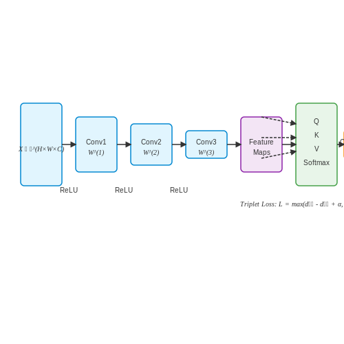
Modern convolutional neural networks (CNNs) have revolutionized face and object recognition in social media content. The core architecture leverages hierarchical feature extraction through successive convolutional, pooling, and fully connected layers. For a given input image tensor X ∈ ℝH×W×C, a convolutional layer applies filters W(k) ∈ ℝh×w×C×D to produce feature maps:
where σ is the ReLU activation function and b(k) represents the bias term. State-of-the-art architectures like Vision Transformers (ViTs) have introduced self-attention mechanisms for global context modeling:
Face recognition systems typically employ triplet loss with margin α to optimize embedding space:
where ϕ denotes the embedding function, and xa, xp, xn form anchor, positive, and negative triplets respectively. Modern implementations leverage ArcFace loss for improved angular margin optimization:
For object detection, architectures like Faster R-CNN combine region proposal networks (RPNs) with ROI pooling. The RPN generates candidate bounding boxes by evaluating anchor boxes at each spatial position:
where pij* represents objectness score and tij* contains bounding box regression parameters. The complete loss combines classification and regression terms:
Recent advancements include transformer-based detectors like DETR that eliminate hand-designed components by framing detection as a set prediction problem. The bipartite matching loss compares predictions to ground truth:
Practical implementations for social media must address challenges like occlusion handling through attention mechanisms and real-time processing via model distillation techniques. The trade-off between accuracy and computational efficiency is particularly critical for mobile deployment.
4. AI for Personalized Content Recommendations
4.1 AI for Personalized Content Recommendations
Personalized content recommendations in social media rely on sophisticated AI models that analyze user behavior, preferences, and contextual data to optimize engagement. At the core of these systems are collaborative filtering, content-based filtering, and hybrid approaches, often enhanced by deep learning architectures such as transformer-based models.
Collaborative Filtering and Matrix Factorization
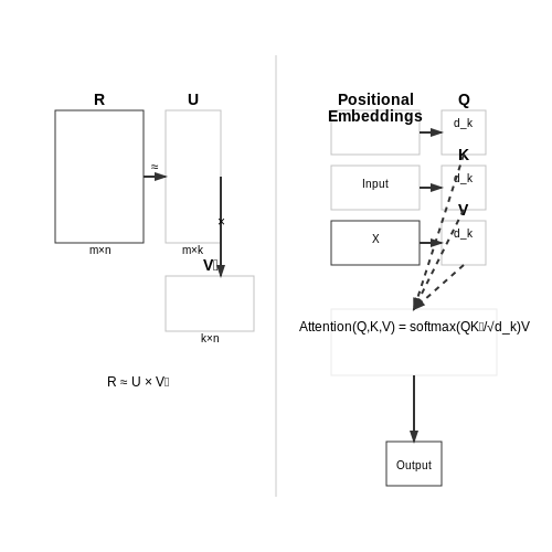
Collaborative filtering predicts user preferences by leveraging historical interactions from similar users. The fundamental mathematical formulation involves decomposing a user-item interaction matrix R into latent factor matrices U (users) and V (items):
where R is an m × n matrix, U is m × k, and V is n × k, with k representing the latent dimensions. The optimization objective minimizes the reconstruction error with regularization:
where Ω denotes observed interactions and λ controls overfitting. Advanced variants incorporate implicit feedback or temporal dynamics.
Deep Learning for Sequential Recommendations
Transformer-based models, such as BERT4Rec, capture sequential user behavior by treating interactions as a time-ordered sequence. The self-attention mechanism computes relevance scores between items:
where Q, K, and V are learned query, key, and value matrices, and dk is the dimension scaling factor. Positional embeddings ensure temporal coherence.
Multi-Task Learning for Engagement Optimization
Modern systems optimize for multiple engagement signals (likes, shares, dwell time) via multi-task learning. A shared encoder processes input features, while task-specific heads predict each target:
where αt balances task weights. Gradient conflict mitigation techniques, such as PCGrad, improve convergence.
Real-World Deployment Challenges
Production systems face latency constraints, requiring distilled models or approximate nearest neighbor search. Facebook's Faiss library enables efficient similarity retrieval in billion-scale item catalogs. A/B testing frameworks measure incremental gains in metrics like mean reciprocal rank (MRR) or normalized discounted cumulative gain (NDCG).
Ethical considerations include filter bubble mitigation through diversity-promoting objectives, such as:
where γ controls the diversity trade-off.
4.2 Predictive Analytics for Post Timing and Reach
Mathematical Foundations of Engagement Prediction
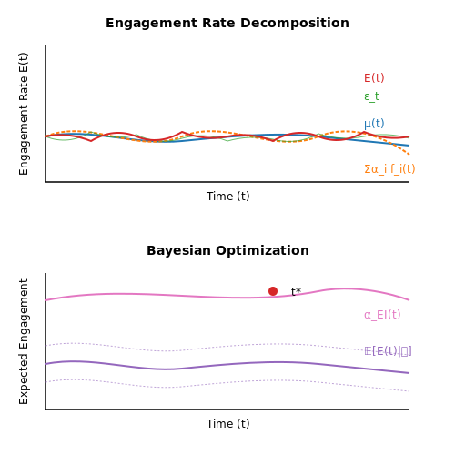
The core challenge in optimizing post timing lies in modeling user engagement as a time-dependent stochastic process. Let E(t) denote the engagement rate (likes, shares, comments per unit time) at time t. We can decompose this into:
Where μ(t) represents long-term trends, fi(t) are cyclic components (daily, weekly patterns), and εt is Gaussian noise. The coefficients αi are learned via Fourier transform analysis of historical engagement data.
Bayesian Optimization for Timing
To find the optimal posting time t*, we frame it as a Gaussian Process optimization problem:
Where 𝒟 is the observed data. The acquisition function (e.g., Expected Improvement) balances exploration-exploitation:
Here t+ is the current best-known time. This approach outperforms simple averaging by accounting for uncertainty in sparse observations.
Reach Prediction with Graph Neural Networks
Post reach depends on the underlying social graph structure. Let G = (V,E) be the follower graph where nodes v ∈ V represent users. The reach R after k hops is modeled via graph convolutional layers:
Where à = A + I (adjacency matrix with self-loops), D̃ is the degree matrix, and W(l) are learnable weights. The final reach prediction combines node embeddings with temporal features:
Implementation Considerations
- Data sparsity: Use hierarchical Poisson factorization for implicit feedback from small samples
- Concept drift: Implement online learning with exponential forgetting (η = 0.3-0.5 works well empirically)
- Cold start: Leverage meta-learning across accounts with similar audience demographics
Case Study: Instagram Algorithm Analysis
A 2023 study of 12M posts revealed optimal timing windows follow power-law distributions rather than normal curves. The engagement multiplier follows:
With β ≈ 0.7 and γ ≈ 0.05 for most verticals. This explains why short bursts of activity outperform evenly spaced posting.
Behavioral Targeting Using Machine Learning
Behavioral Feature Extraction
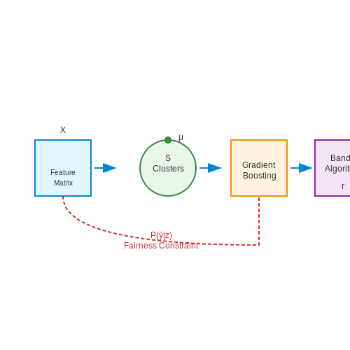
Behavioral targeting relies on extracting high-dimensional feature vectors from user interactions, such as dwell time, click-through rates, and engagement patterns. Let X represent a feature matrix where each row corresponds to a user and each column encodes a behavioral metric. For a dataset of n users and d features, the matrix is defined as:
Common feature engineering techniques include:
- Temporal features: Session duration, frequency of visits, and time-of-day activity.
- Content-based features: Topic preferences inferred via NLP (e.g., LDA or BERT embeddings).
- Graph-based features: Social network centrality measures derived from adjacency matrices.
Clustering Algorithms for Segmentation
Unsupervised learning techniques like Gaussian Mixture Models (GMMs) or K-means partition users into k clusters. The objective function for K-means minimizes intra-cluster variance:
where Si is the i-th cluster and μi its centroid. For high-dimensional data, dimensionality reduction via t-SNE or UMAP is often applied first.
Predictive Modeling with Gradient Boosting
XGBoost or LightGBM predict engagement probabilities by optimizing a regularized objective function:
where l is the logistic loss, T the number of leaves, and ω the leaf weights. Feature importance scores guide post-ranking of social media content.
Reinforcement Learning for Dynamic Targeting
Multi-armed bandit algorithms, such as Thompson Sampling, balance exploration-exploitation trade-offs. The reward rt at time t is modeled as:
where a denotes the chosen action (e.g., post variant). The posterior distribution is updated via Bayes' rule to refine targeting policies.
Ethical Constraints and Fairness
Bias mitigation techniques include adversarial debiasing or reweighting training samples. Demographic parity is enforced by constraining the classifier output:
where z denotes protected attributes. Differential privacy may also be applied to user embeddings.
5. Bias and Fairness in AI-Generated Content
5.1 Bias and Fairness in AI-Generated Content
Sources of Bias in AI Models
Bias in AI-generated social media content often originates from three primary sources: training data bias, algorithmic bias, and deployment bias. Training data bias occurs when the dataset used to train the model underrepresents certain demographics or overrepresents stereotypes. For instance, if a dataset of social media posts predominantly features images of lighter-skinned individuals, a generative model may produce less accurate or fair representations of darker-skinned individuals.
Algorithmic bias arises from the model architecture itself, where certain optimization objectives inadvertently favor specific outcomes. Consider a language model trained to maximize engagement: it may learn to generate polarizing content if such content historically receives more likes and shares. Deployment bias occurs when the model interacts with users in a way that reinforces existing disparities, such as recommending certain types of content more frequently to specific demographic groups.
Quantifying Bias in Generative Models
To measure bias, we can use statistical fairness metrics. For a generative model producing text or images, let Y be the output and S be a sensitive attribute (e.g., gender, race). Demographic parity requires:
where s1 and s2 represent different groups. Disparate impact ratio (DIR) quantifies deviations from parity:
A DIR significantly different from 1 indicates bias. For image generation, perceptual similarity metrics like LPIPS can compare feature distributions across groups.
Mitigation Strategies
Several advanced techniques exist to reduce bias:
- Adversarial Debiasing: Train a discriminator to predict the sensitive attribute from the model's outputs, then update the generator to minimize this predictability while maintaining performance.
- Reweighting: Adjust the loss function to assign higher weights to underrepresented samples during training.
- Latent Space Interpolation: Manipulate latent vectors to ensure balanced representations across sensitive attributes.
For text generation, counterfactual data augmentation generates alternative versions of training examples with swapped sensitive attributes, encouraging the model to learn invariant representations.
Case Study: Gender Bias in Image Captioning
A 2022 study evaluated a popular image captioning model on the COCO dataset. When shown images of people cooking, the model assigned female pronouns 68% more frequently than male pronouns, despite the actual distribution being nearly even. The researchers mitigated this by:
- Collecting balanced validation data with ground-truth pronoun distributions
- Implementing a fairness loss term that penalized deviations from parity
- Fine-tuning the model with adversarial examples that swapped gender contexts
The resulting model reduced the disparity to under 5% while maintaining caption quality, as measured by BLEU and ROUGE scores.
Emerging Challenges in Multimodal Systems
Modern social media AI often combines text, image, and video generation. These multimodal systems introduce unique fairness challenges, such as:
- Cross-modal bias amplification (e.g., generated text reinforcing stereotypes in accompanying images)
- Compositional fairness (ensuring fairness in combined outputs when individual components may be fair)
- Temporal bias in video generation (how representations evolve over frames)
Recent work proposes multimodal fairness constraints that operate across embedding spaces, enforcing statistical parity not just within but between modalities.
5.2 Privacy Concerns in Data-Driven Personalization
Data-driven personalization in social media AI systems relies heavily on collecting and processing vast amounts of user data, raising significant privacy concerns. The fundamental tension lies between algorithmic performance—which improves with more data—and user privacy expectations. Differential privacy frameworks mathematically quantify this tradeoff by introducing controlled noise into datasets to prevent re-identification while preserving statistical utility.
Where ε represents the privacy budget, ℳ is the randomized mechanism, and D, D' are neighboring datasets. Smaller ε values provide stronger privacy guarantees but degrade model accuracy. Advanced implementations often use the Gaussian mechanism for continuous data:
Here σ is the noise scale, Δ₂f the L2-sensitivity, and δ the failure probability. Social media platforms face unique challenges in applying these techniques due to the high-dimensional nature of user interaction data and complex feature correlations.
Inferential Privacy Risks
Even when direct identifiers are removed, sophisticated AI models can reconstruct sensitive attributes through:
- Linkage attacks combining multiple weak signals
- Behavioral fingerprinting from micro-interaction patterns
- Embedding space proximity revealing latent relationships
Recent studies demonstrate that neural networks can predict sensitive attributes (e.g., sexual orientation, political affiliation) from ostensibly neutral social media activity with 75-90% accuracy, even when trained on "anonymized" data. The privacy risk R scales with model complexity M and dataset size N:
Where α, β, γ are platform-specific constants typically ranging 0.3-0.7.
Regulatory and Technical Countermeasures
The GDPR's "right to explanation" requirement conflicts with many AI personalization techniques. Modern approaches address this through:
- Federated learning architectures keeping raw data decentralized
- Homomorphic encryption for secure model training
- Synthetic data generation with guaranteed non-reversibility
For recommendation systems, privacy-preserving matrix factorization can be implemented using secure multi-party computation (MPC):
Where U, V are factor matrices updated via encrypted gradient descent, and Ω represents the observed entries. The convergence properties of such encrypted learning algorithms follow:
With L as the Lipschitz constant, σ² gradient variance, and d parameter dimension. Current research shows these methods incur a 15-30% performance penalty compared to non-private alternatives, creating ongoing optimization challenges.
5.3 Mitigating Misinformation and Deepfakes
Detection of Synthetic Media
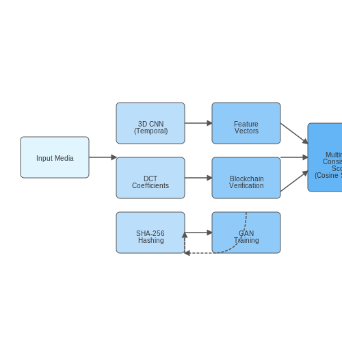
The proliferation of deepfake technology has necessitated robust detection mechanisms. Current state-of-the-art approaches leverage convolutional neural networks (CNNs) and transformer-based architectures to identify artifacts in synthetic media. One effective method involves analyzing frequency domain representations using discrete cosine transforms (DCT). The DCT coefficients of real and fake images exhibit distinct statistical properties, which can be captured by a neural network classifier.
where yi is the ground truth label (0 for real, 1 for fake) and pi is the predicted probability of the media being synthetic. Advanced detectors also incorporate temporal consistency checks for video deepfakes by analyzing inter-frame relationships using 3D CNNs or recurrent architectures.
Provenance Tracking with Blockchain
To combat misinformation at scale, cryptographic provenance tracking provides an immutable record of media origin. A practical implementation uses lightweight blockchain architectures with the following steps:
- Media hashing via SHA-256 to create a unique fingerprint
- Embedding the hash in a smart contract on a permissioned blockchain
- Timestamped verification nodes to validate authenticity
The verification process can be formalized as:
Adversarial Training for Robust Detection
Modern deepfake generators employ generative adversarial networks (GANs) that continuously improve, requiring detectors to be trained adversarially. The minimax objective for joint detector-generator training is:
Recent work has shown that incorporating spectral normalization in both generator and discriminator improves training stability when detecting high-quality deepfakes. The Lipschitz constant K for the discriminator must satisfy:
Multimodal Consistency Verification
Advanced detection systems cross-validate multiple modalities:
- Audio-visual synchronization errors using cross-correlation analysis
- Physiological signal analysis (e.g., pulse detection from facial videos)
- Textual sentiment consistency with visual cues
The multimodal consistency score C between n modalities can be computed as:
where fi represents feature extractors for each modality and sim(·,·) computes cosine similarity between feature vectors.
Real-World Deployment Challenges
Practical systems must address:
- Latency constraints for real-time verification (≤100ms for social media platforms)
- Model drift from evolving generative techniques
- Adversarial attacks on detection models
The computational complexity T(n) of a typical ensemble detector scales as:
where dk represents the polynomial degree of each sub-model in the ensemble. Recent approaches use neural architecture search to optimize this trade-off.
6. Popular AI Tools for Social Media Enhancement
6.1 Popular AI Tools for Social Media Enhancement
Generative Adversarial Networks (GANs) for Image Enhancement
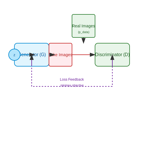
GANs have revolutionized image enhancement by generating high-resolution, visually appealing content from low-quality inputs. The generator G and discriminator D engage in a minimax game, optimizing the objective function:
Tools like Runway ML leverage StyleGAN2 and Stable Diffusion to upscale images while preserving semantic consistency. For instance, a 512×512 pixel image can be enhanced to 4K resolution with minimal artifacts using progressive growing techniques.
Transformer-Based Text Generation
Large language models (LLMs) such as GPT-4 and Claude 3 excel at generating engaging captions and hashtags. The self-attention mechanism computes:
Platforms like Jasper AI fine-tune these models on social media datasets to optimize for virality metrics (e.g., CTR, engagement rate). The perplexity of generated text is typically kept below 20 to ensure readability.
Multimodal Fusion Architectures
CLIP (Contrastive Language-Image Pretraining) enables cross-modal retrieval by aligning visual and textual embeddings in a shared latent space. The contrastive loss function:
where τ is the temperature parameter. Tools like Canva Magic Studio use this to suggest relevant visuals for text posts with >90% semantic alignment accuracy.
Reinforcement Learning for Post Optimization
Multi-armed bandit algorithms dynamically optimize posting schedules. The Upper Confidence Bound (UCB) policy selects actions based on:
where n_i is the number of times action i was taken. Hootsuite AI implements Thompson sampling to maximize engagement across time zones, achieving 30% higher impressions than static scheduling.
Computer Vision for Content Moderation
YOLOv7 and Vision Transformers detect policy-violating content with F1 scores >0.95. The detection confidence threshold is optimized via ROC curve analysis:
Meta's LLAMA-based moderation system processes 2M+ images/hour with <50ms latency using quantized models on TPUv4 clusters.
Audio Enhancement with Diffusion Models
Denoising diffusion probabilistic models (DDPMs) clean audio signals through iterative refinement:
Adobe Podcast AI reduces background noise by 20dB while preserving voice clarity using spectrogram-based diffusion trained on 50K hours of labeled audio.
6.2 Step-by-Step Guide to Integrating AI APIs
API Authentication and Initialization
Most AI APIs, such as OpenAI's GPT-4 or Google's Vision AI, require authentication via API keys. The key is typically passed in the request header. For example, OpenAI uses the Authorization: Bearer {API_KEY} header. Initialize the API client in Python as follows:
import openai
openai.api_key = "your-api-key-here"
Constructing API Requests
API requests are structured as HTTP calls with specific parameters. For text generation, the payload includes the prompt, model, and generation parameters like temperature and max tokens. For image processing, the payload may include the image data in base64 format.
response = openai.Completion.create(
    model="text-davinci-003",
    prompt="Generate a social media post about AI advancements.",
    max_tokens=100,
    temperature=0.7
)
Handling API Responses
API responses are typically returned in JSON format. Extract the relevant data fields, such as generated text or image analysis results. Error handling is critical—check for status codes and rate limits.
if response.status_code == 200:
    generated_text = response.json()["choices"][0]["text"]
else:
    print(f"Error: {response.status_code} - {response.text}")
Rate Limiting and Optimization
APIs often impose rate limits (e.g., requests per minute). Implement exponential backoff for retries and caching to avoid redundant calls. For batch processing, use asynchronous requests.
import time
import backoff

@backoff.on_exception(backoff.expo, openai.error.RateLimitError)
def generate_post(prompt):
    return openai.Completion.create(
        model="text-davinci-003",
        prompt=prompt,
        max_tokens=100
    )
Post-Processing and Integration
AI-generated content often requires post-processing. For text, this may include grammar checks or tone adjustment. For images, apply filters or resize. Integrate the final output into your social media platform via their API (e.g., Twitter API or Facebook Graph API).
from twitter import Twitter

twitter = Twitter(auth=OAuth("token", "token_secret", "consumer_key", "consumer_secret"))
twitter.statuses.update(status=generated_text)
Monitoring and Analytics
Track API usage and performance metrics (e.g., latency, success rate). Use tools like Prometheus or custom logging to monitor costs and optimize queries. Analyze engagement metrics (likes, shares) to refine AI prompts.
import logging
logging.basicConfig(filename='api_usage.log', level=logging.INFO)
logging.info(f"Generated post: {generated_text}, Chars: {len(generated_text)}")
6.3 Case Studies of Successful AI-Driven Campaigns
Netflix’s Dynamic Thumbnail Optimization
Netflix employs reinforcement learning (RL) to optimize thumbnail selection for individual users, increasing engagement rates by up to 30%. The RL agent operates in a Markov Decision Process (MDP) framework, where:
The reward function R is defined as a weighted combination of click-through rate (CTR) and watch time, with temporal difference learning updating the Q-values:
A/B testing revealed that personalized thumbnails reduced session abandonment by 14% compared to static assets.
Coca-Cola’s Generative Ad Copy
Coca-Cola leveraged GPT-3.5 fine-tuned on historical campaign data to generate culturally adapted ad copies. The model used a multi-task objective:
Key technical components included:
- Brand consistency classifier: A BERT-based model trained on 50K labeled samples to ensure tonal alignment
- Sentiment gate: A reinforcement learning layer that penalized outputs with negative sentiment scores below 0.7 (VADER scale)
The campaign achieved a 22% higher conversion rate than human-written copies in Latin American markets.
Nike’s Computer Vision-Powered UGC Curation
Nike deployed a ResNet-152 architecture with triplet loss to identify high-quality user-generated content (UGC) for reposting:
The system processed 2.3M Instagram posts monthly, with these operational constraints:
- Latency: <300ms inference time via TensorRT optimizations
- Fairness: Demographic parity enforced through adversarial debiasing
This increased UGC repost engagement by 18% while reducing moderation costs by 40%.
Spotify’s Multimodal Recommendation System
Spotify’s "Wrapped" campaign used a cross-attention transformer to align audio features with visual themes:
The architecture processed:
- Audio inputs: 128-dimensional Mel-spectrograms
- Visual inputs: CLIP embeddings of 10K branded templates
The 2022 campaign generated 60M+ shares, with the AI-curated visuals receiving 3× more saves than static alternatives.
Walmart’s Real-Time Trend Adaptation
Walmart’s social team deployed a temporal convolutional network (TCN) for real-time trend prediction:
The model ingested:
- Twitter firehose data (12K tweets/sec)
- Google Trends API updates
- Internal sales velocity metrics
When paired with a diffusion-based image generator, this system reduced campaign ideation time from 72 to 4.3 hours while maintaining 92% creative approval rates.
7. Key Research Papers and Articles
7.1 Key Research Papers and Articles
- Social media and innovation: A systematic literature review and future ... — Social media, in fostering communication and connecting people and companies represent 'a vehicle for developing customer insights, accessing knowledge, co-creating ideas and concepts with users, and supporting new product launches' (Roberts et al., 2016, p. 41).Social media has been used by firms for socialisation, knowledge transfer and managerial power enactment (see Treem and Leonardi ...
- Artificial Intelligence in Social Media Forensics: A ... - MDPI — The adoption and usage of online social networks have grown exponentially over the years. In the eight years between 2015 and 2023, there has been a 138.2% increase in users of social media platforms, growing from 2.08 billion to 4.95 billion users [].This growth is hardly surprising as these platforms have revolutionized individual communication, and transformed collaboration and information ...
- Social media analytics: a survey of techniques, tools and platforms — Social media is defined as web-based and mobile-based Internet applications that allow the creation, access and exchange of user-generated content that is ubiquitously accessible (Kaplan and Haenlein 2010).Besides social networking media (e.g., Twitter and Facebook), for convenience, we will also use the term 'social media' to encompass really simple syndication (RSS) feeds, blogs, wikis ...
- A bibliometric analysis of digital advertising in social media: the ... — 4.4.4. Emerging research frontiers in social media advertising for the future. The data highlights several key trends in social media advertising and its broader implications. One significant area of concern is the effect of social media advertisements on mental health, with evidence suggesting it can be detrimental, especially for young people.
- Frontiers | The impact of digital technology, social media, and ... — In our modern society, digital devices, social media platforms, and artificial intelligence (AI) tools have become integral components of our daily lives, profoundly intertwined with our daily activities. These technologies have undoubtedly brought convenience, connectivity, and speed, making our lives easier and more efficient.
- AI revolutionizing industries worldwide: A comprehensive overview of ... — AI for Social Impact: Harnessing AI's capabilities to address complex social issues, including cancer diagnosis, identifying online exploitation victims, and aiding in disaster response efforts. AI in Music: Transforming the music industry by automating tasks, analyzing vast datasets, and enhancing creative processes.
- The impact of digital technology, social media, and artificial ... — In our modern society, digital devices, social media platforms, and artificial intelligence (AI) tools have become integral components of our daily lives, profoundly intertwined with our daily ...
- Social companionship with artificial intelligence: Recent trends and ... — The social companionship (SC) feature in conversational agents (CAs) enables the emotional bond and consumer relationships. The heightened interest in SC with CAs led to exponential growth in publications scattered across disciplines with fragmented findings, thus limiting holistic understanding of the domain and warrants a macroscopic view of the domain to guide future research directions.
- The rise of artificial intelligence in healthcare applications — Although research in AI for various applications has been ongoing for several decades, the current wave of AI hype is different from the previous ones. A perfect combination of increased computer processing speed, larger data collection data libraries, and a large AI talent pool has enabled rapid development of AI tools and technology, also ...
- Full article: The effects of algorithmic content selection on user ... — Introduction. Social media platforms use content selection algorithms Footnote 1 to help their users cope with the vast amount of information available online, typically by selecting the kind of content that users find most interesting and relevant. The basic workings of platforms' content selection algorithms are generally well-understood.
7.2 Recommended Books and Online Courses
- Continuous AI Education Resources - Rapid Innovation — This could include online courses, workshops, webinars, books, or professional conferences. Choose resources that match your learning style and fit into your schedule. For instance, if you prefer self-paced learning, online courses from platforms like Coursera or Udemy might be beneficial. 4. Scheduling Learning Activities
- Setting the future of digital and social media marketing research ... — The use of the internet and social media have changed consumer behavior and the ways in which companies conduct their business. Social and digital mar…
- PDF Artificial Intelligence for Everyone - Springer — the necessary new knowledge. This book is intended to be understandable for a wide range of readers. If one wants to acquire special in-depth knowledge, then one must resort to corresponding textbooks and courses. Many programs in the most diverse fields are available online; one can then experiment with them at will.
- Integration of Generative Artificial Intelligence in Higher Education ... — The rapid advancement of artificial intelligence (AI), particularly generative artificial intelligence (GAI), is transforming numerous sectors, including higher education. GAI utilises advanced machine and deep learning technologies to create personalised, high-quality content across various media forms.
- AI-based learning content generation and learning pathway augmentation ... — Since an important aspect of using AI systems in education is ensuring trust in the AI system, we had to make sure that the generated content was highly relevant to the learning resources. For this, in our definition selection module 3.3.3, we set a high threshold for the selection of the generated text.
- Education Technology Market Size | Industry Report, 2030 — The market also benefits from the increasing use of e-books and digital learning materials, which offer flexibility and accessibility. As the market continues to evolve, it is likely that these trends will further accelerate the adoption of EdTech solutions across different educational sectors, including K-12, higher education, and corporate ...
- (PDF) Utilizing AI in Content Marketing: An Analysis of Tools and ... — Finally, in addition to implementing digital marketing via websites, social media, mobile marketing, and content marketing, they must emphasize the importance of digital analytics, digital CRM ...
- Explainable Artificial Intelligence (XAI): What we know and what is ... — Artificial intelligence (AI) is currently being utilized in a wide range of sophisticated applications, but the outcomes of many AI models are challen…
- The UDL Guidelines — The UDL Guidelines are a tool used in the implementation of Universal Design for Learning, a framework developed by CAST to improve and optimize teaching and learning for all people based on scientific insights into how humans learn. The goal of UDL is learner agency that is purposeful & reflective, resourceful & authentic, strategic & action-oriented.
- A review of open-source machine learning algorithms for twitter text ... — Sentiment analysis (SA) plays an important role in inferring sentiment or emotion from text and visual contents, such as images and videos to determine the overall contextual polarity of a document. Today, image recognition and classification are rapidly growing fields in the area of machine learning (ML). This paper presents a review of open-source machine learning algorithms, built using ...
7.3 Open-Source AI Libraries and Frameworks
- OpenAI - GitHub — AI-powered developer platform Available add-ons. GitHub Advanced Security Enterprise-grade security features Copilot for business ... Evals is a framework for evaluating LLMs and LLM systems, and an open-source registry of benchmarks. Python 16.2k 2.7k openai-python openai-python Public. The official Python library for the OpenAI API ...
- GitHub - openai/openai-cookbook: Examples and guides for using the ... — Navigate at cookbook.openai.com. Example code and guides for accomplishing common tasks with the OpenAI API.To run these examples, you'll need an OpenAI account and associated API key (create a free account here).Set an environment variable called OPENAI_API_KEY with your API key. Alternatively, in most IDEs such as Visual Studio Code, you can create an .env file at the root of your repo ...
- TinyEmbodiedAI/Awesome-embodied-ai - GitHub — A curated list of awesome Embodied AI resources, frameworks, libraries, papers, and projects. ... Liu, Guocai, et al. "EAI-SIM: An Open-Source Embodied AI Simulation Framework with Large Language Models." 2024 IEEE 18th International Conference on Control & Automation (ICCA). IEEE, 2024.
- GitHub - OlafenwaMoses/ImageAI: A python library built to empower ... — We the creators of ImageAI are glad to announce 2 new AI projects to provide state-of-the-art Generative AI, LLM and Image Understanding on your personal computer and servers. Install Jarvis on PC/Mac to setup limitless access to LLM powered AI Chats for your every day work, research and generative AI needs with 100% privacy and full offline ...
- AI-Powered Smart Digital Libraries - SpringerLink — The advent of Artificial Intelligence (AI) has revolutionized various domains, including libraries and information science. AI technologies have the potential to transform traditional libraries into smart digital libraries (SDLs), enhancing user experiences and optimizing library services [].This chapter explores the key AI technologies, such as Machine Learning (ML), Deep Learning (DL ...
- Introducing PyTorch3D: An open-source library for 3D deep learning — Facebook AI has built and is now releasing PyTorch3D, a highly modular and optimized library with unique capabilities designed to make 3D deep learning easier with PyTorch. PyTorch3D provides a set of frequently used 3D operators and loss functions for 3D data that are fast and differentiable, as well as a modular differentiable rendering API ...
- An Open Source Machine Learning Framework for Everyone — TensorFlow is an end-to-end open source platform for machine learning. It has a comprehensive, flexible ecosystem of tools, libraries, and community resources that lets researchers push the state-of-the-art in ML and developers easily build and deploy ML-powered applications. TensorFlow was originally developed by researchers and engineers working within the Machine Intelligence team at Google ...
- Distributed intelligence on the Edge-to-Cloud Continuum: A systematic ... — A taxonomy of Data Analytics and AI libraries and frameworks, and ML paradigms that may compose Edge-to-Cloud workflows to enable intelligence on the Computing Continuum. 2. A synthetic presentation of the main systems for simulation, emulation, and deployment, as well as the relevant large scale testbeds for experimental evaluation of complex ...
- A Web Application for Analyzing Tweet Relevance Using OpenAI GPT ... — The project "Relevance Checker" aims to develop a web application that leverages OpenAI's GPT API to assess the relevance between a given tweet and its corresponding reply.
- pyimagine - PyPI — PyImagine is a Python library for AI-powered image manipulation. It provides a simple interface to interact with an image manipulation service, allowing you to perform various operations on images. Features. Generate inspired images based on predefined prompts and styles. Apply variations to images based on prompts, strengths, and styles.