

AI-Powered Learning Recommendation Systems
1. Core Concepts and Definitions
1.1 Core Concepts and Definitions
Formal Definition of Recommendation Systems
Recommendation systems are algorithmic frameworks designed to predict user preferences by analyzing behavioral patterns, historical interactions, and contextual data. Mathematically, given a set of users U and items I, the system learns a utility function f: U × I → R, where R represents a relevance score. The goal is to approximate:
where rui is the predicted relevance of item i to user u. In AI-powered learning systems, i typically represents educational content (e.g., courses, articles, exercises).
Taxonomy of Recommendation Methods
Modern systems employ hybrid approaches, but foundational techniques include:
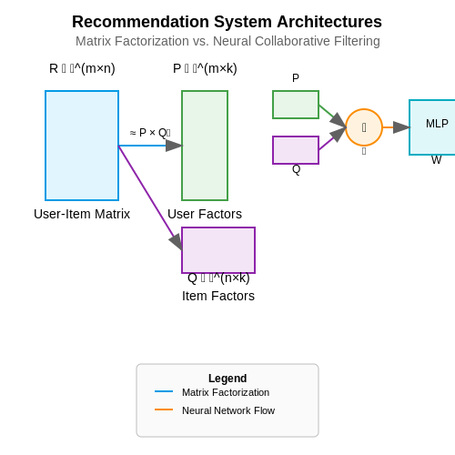
- Collaborative Filtering (CF): Leverages user-item interaction matrices to identify latent patterns. Matrix factorization decomposes the sparse matrix R ∈ ℝm×n into user and item latent factors P ∈ ℝm×k and Q ∈ ℝn×k by minimizing:
- Content-Based Filtering: Utilizes item features xi and user profiles θu to compute cosine similarity or train classifiers (e.g., logistic regression).
- Knowledge-Based: Incorporates domain-specific constraints (e.g., prerequisite dependencies in learning paths).
AI Enhancements in Learning Systems
Deep learning architectures address sparsity and cold-start problems in educational contexts:
- Neural Collaborative Filtering (NCF): Replaces matrix factorization with neural networks to model non-linear interactions:
where ϕ is a multi-layer perceptron and ⊕ denotes concatenation.
- Transformer-Based Sequential Recommendations: Models temporal dynamics of learning activities using self-attention mechanisms, capturing long-range dependencies in interaction sequences.
Evaluation Metrics
Performance is quantified through ranking and accuracy metrics:
- Normalized Discounted Cumulative Gain (nDCG): Measures ranking quality with position-aware discounts:
- Mean Reciprocal Rank (MRR): Computes the inverse rank of the first relevant item in recommendations.
Contextual Adaptation
Modern systems integrate contextual features (e.g., learning pace, device type) via tensor factorization or attention mechanisms. A contextualized relevance score extends the utility function to f: U × I × C → R, where C represents contextual dimensions.
Key Components of Recommendation Systems
Data Representation and Feature Engineering
Recommendation systems rely on structured representations of users, items, and interactions. For a user-item matrix R of dimensions m × n, where m is the number of users and n is the number of items, entries Rij represent explicit feedback (e.g., ratings) or implicit feedback (e.g., clicks). Feature engineering transforms raw data into meaningful representations:
Here, X and Y are latent factor matrices for users and items, respectively, with d dimensions. Techniques like TF-IDF, word embeddings, or graph-based features augment sparse interaction data.
Collaborative Filtering (CF) Algorithms
CF methods predict user preferences by leveraging historical interactions. Matrix factorization decomposes R into low-rank approximations:
where Ω denotes observed entries, and λ controls regularization. Alternating Least Squares (ALS) or Stochastic Gradient Descent (SGD) optimize this objective. Deep learning variants replace dot products with neural architectures.
Content-Based Filtering
Content-based systems match item attributes to user profiles. For textual data, cosine similarity between TF-IDF vectors determines relevance:
Advanced implementations use BERT or Transformer embeddings for semantic matching. Hybrid models combine CF and content-based signals to mitigate cold-start problems.
Evaluation Metrics
Performance is quantified using ranking and prediction metrics:
- Precision@k: Proportion of relevant items in top-k recommendations.
- NDCG@k: Discounted cumulative gain normalized by ideal ranking.
- RMSE: Root mean squared error for rating prediction tasks.
A/B testing in production systems measures business metrics like click-through rate (CTR) or conversion rate.
Scalability and Real-Time Processing
Large-scale systems employ approximate nearest neighbor (ANN) search via locality-sensitive hashing (LSH) or FAISS. Streaming architectures (e.g., Apache Flink) update models incrementally using event-time processing.
# Example: Incremental matrix factorization with PySpark
from pyspark.ml.recommendation import ALS
als = ALS(
   rank=10,
   maxIter=5,
   regParam=0.01,
   implicitPrefs=True,
   coldStartStrategy="drop"
)
model = als.fit(streaming_df)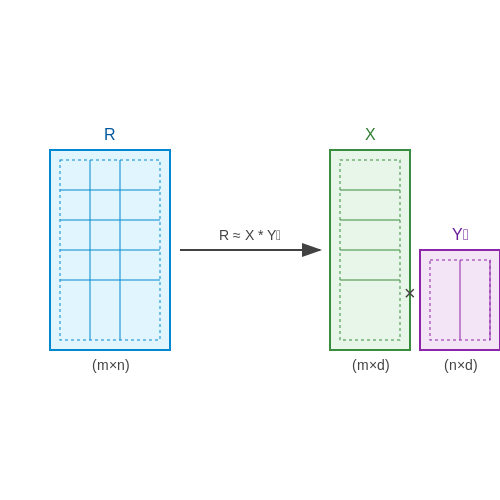
1.3 Types of Recommendation Algorithms in Education
Collaborative Filtering
Collaborative filtering (CF) operates on the principle that users who agreed in the past will agree in the future. In educational contexts, this translates to recommending learning materials based on the preferences of similar learners. The approach can be user-based or item-based. User-based CF identifies learners with similar interaction patterns, while item-based CF recommends items similar to those a learner has previously engaged with.
The core mathematical formulation for user-based CF involves computing the similarity between users, often using Pearson correlation or cosine similarity. For users u and v, the Pearson correlation coefficient is given by:
where Iuv represents items rated by both users, rui is the rating of item i by user u, and r̄u is the average rating of user u. Predictions for unrated items are then generated using a weighted average of ratings from similar users.
Content-Based Filtering
Content-based filtering (CBF) recommends items by matching their features to a learner's profile. In education, this involves analyzing metadata such as topic, difficulty level, and resource type. A vector space model represents both learners and items, with recommendations generated based on cosine similarity between vectors.
The learner profile L and item profile I are typically represented as TF-IDF vectors:
where L·I denotes the dot product and ||L||, ||I|| are the Euclidean norms. Advanced implementations may incorporate latent semantic indexing (LSI) or word embeddings to capture semantic relationships between educational materials.
Knowledge-Based Recommendation
Knowledge-based systems employ explicit domain knowledge to make recommendations, making them particularly suitable for structured learning paths in education. These systems often use constraint-based or case-based reasoning. Constraint-based approaches define hard rules (e.g., prerequisite relationships between courses), while case-based reasoning retrieves similar learning scenarios from a knowledge base.
A constraint-based system can be formalized as a set of rules R and constraints C:
where c(u, i) evaluates whether item i satisfies constraint c for user u. These systems excel in scenarios requiring pedagogical structure, such as curriculum sequencing.
Hybrid Approaches
Hybrid recommendation systems combine multiple techniques to mitigate individual limitations. Common hybridization strategies in educational contexts include:
- Weighted hybridization: Linearly combines scores from different algorithms
- Feature augmentation: Uses output from one algorithm as input to another
- Meta-level hybridization: Employs one model to generate input for another
A weighted hybrid system might combine collaborative and content-based scores as:
where α is a tunable parameter controlling the influence of each component. Modern implementations increasingly leverage deep learning to learn optimal combination strategies automatically.
Reinforcement Learning for Adaptive Recommendations
Reinforcement learning (RL) frameworks model the recommendation process as a Markov decision process (MDP), where the system learns optimal recommendation policies through interaction. In educational settings, states represent learner knowledge states, actions correspond to recommendation choices, and rewards reflect learning outcomes.
The Q-learning update rule for this MDP is:
where st is the current state, at the chosen action, rt+1 the immediate reward, and γ the discount factor. Deep Q-networks (DQN) extend this approach to handle high-dimensional state spaces common in educational applications.
2. Data Sources for Learning Recommendations
Data Sources for Learning Recommendations
Effective AI-powered learning recommendation systems rely on diverse, high-quality data sources to generate personalized suggestions. The choice of data directly impacts the system's ability to model user preferences, learning objectives, and content relevance. Below, we categorize and analyze the primary data sources used in modern recommendation engines.
User Interaction Data
Implicit and explicit feedback from learners forms the backbone of personalized recommendations. Implicit signals include:
- Clickstream data: Time spent on resources, navigation paths, and interaction frequency.
- Engagement metrics: Video watch completion rates, quiz attempts, and annotation activity.
- Session duration: Temporal patterns in learning behavior.
Explicit feedback mechanisms include:
- Ratings (1-5 scales or thumbs up/down)
- Self-reported difficulty levels
- Manual tagging of interests/skills
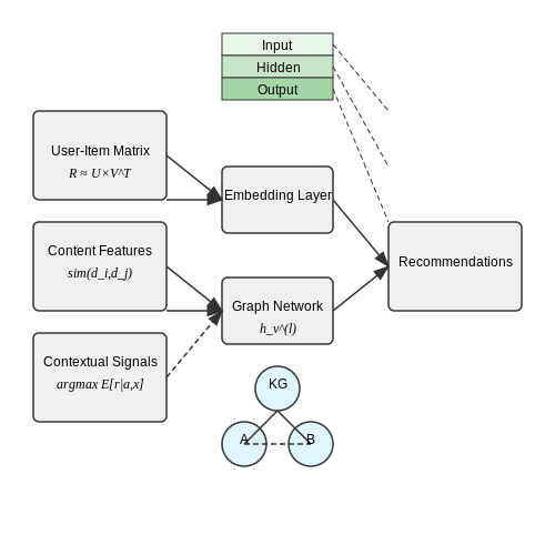
These data streams are typically modeled using collaborative filtering approaches, where the user-item interaction matrix R is decomposed into latent factors:
where U represents user embeddings and V contains item embeddings in a shared latent space.
Content Metadata
Structured information about learning resources enables content-based recommendations:
- Taxonomic classifications: Subject hierarchies (e.g., ACM Computing Classification System)
- Pedagogical attributes: Difficulty level, prerequisite requirements, learning objectives
- Multimodal features: Text embeddings from transcripts, visual features from video frames
For text-based resources, TF-IDF or BERT embeddings create content representations:
where di and dj are documents represented by their embedding vectors.
Contextual Signals
Temporal, spatial, and device context significantly impact recommendation relevance:
- Temporal patterns: Time-of-day preferences, learning session frequency
- Location data: Geographic preferences for localized content
- Device characteristics: Mobile vs desktop consumption patterns
Contextual bandit algorithms often model these dynamics:
where action a (recommendation) is chosen based on context x to maximize expected reward r.
Knowledge Graphs
Structured knowledge representations connect learning resources through:
- Prerequisite relationships
- Concept dependencies
- Skill ontologies
Graph neural networks propagate user preferences through these structures:
where hv(l) is the node representation at layer l, N(v) denotes neighbors, and cuv is a normalization constant.
Psychometric Data
Cognitive and affective states derived from:
- Eye-tracking measurements
- Keystroke dynamics
- Physiological sensors (EEG, GSR)
These require specialized fusion architectures:
where sensor inputs xt are processed through recurrent layers with attention mechanisms.
2.2 Feature Engineering for Educational Data
Feature engineering transforms raw educational data into meaningful predictors that enhance the performance of recommendation systems. Unlike generic datasets, educational data exhibits unique temporal, sequential, and hierarchical structures that require specialized techniques.
Temporal Feature Extraction
Learning behaviors follow non-stationary patterns influenced by deadlines, course schedules, and forgetting curves. Key temporal features include:
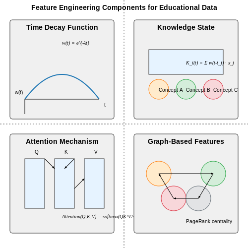
- Time decay-weighted activity counts: Recent interactions receive higher weights using exponential decay:
$$ w(t) = e^{-\lambda(t_{current} - t_{event})} $$where λ controls the decay rate (typically 0.01-0.05 for weekly granularity).
- Periodic patterns: Fourier transforms extract daily/weekly study cycles from timestamp sequences.
- Pacing deviation: Measures alignment between actual and recommended study intervals using dynamic time warping.
Knowledge State Modeling
Representing learners' knowledge requires modeling the forgetting process and concept dependencies:
where K_i is knowledge of concept i, α_j is learning gain from interaction j, β_j is the forgetting rate, and I_ij indicates concept coverage.
Bayesian Knowledge Tracing (BKT) parameters can be repurposed as features when interpretability is prioritized over accuracy.
Behavioral Sequence Encoding
Transformer architectures have demonstrated superior performance in encoding action sequences compared to traditional Markovian approaches. For a sequence of length N:
where queries (Q), keys (K), and values (V) are learned embeddings of activity types, duration, and outcomes. The [CLS] token embedding serves as a fixed-dimensional sequence representation.
Graph-Based Feature Construction
Prerequisite networks and concept maps enable topological feature extraction:
- Node centrality: Measures concept importance via PageRank or betweenness centrality
- Propagation features: Simulate knowledge diffusion using personalized PageRank with damping factor α=0.85
- Community detection: Identifies interdisciplinary connections through Louvain modularity
Feature Selection Techniques
High-dimensional educational features require rigorous selection to prevent overfitting:
where J is the joint mutual information criterion that balances relevance (I(X;Y)) and redundancy (I(X;X_j)). For temporal features, Granger causality tests establish predictive relationships.
Recursive feature elimination with cross-validation (RFECV) using SHAP values provides robust rankings for tree-based models, while ℓ1-regularized logistic regression works well for linear approaches.
2.3 Handling Implicit vs. Explicit Feedback
Learning recommendation systems rely heavily on user feedback to refine their models. Feedback can be broadly categorized into explicit and implicit forms, each presenting unique challenges and opportunities for algorithmic processing. Understanding the distinction is critical for designing robust recommendation engines.
Explicit Feedback
Explicit feedback consists of direct user-provided ratings, such as star ratings, thumbs-up/down, or written reviews. This data is structured and unambiguous, making it easier to incorporate into traditional collaborative filtering or matrix factorization techniques. The key advantage is its interpretability: a 5-star rating clearly indicates strong preference, while a 1-star rating signals dissatisfaction.
Here, \( R_{ui} \) represents the observed rating by user \( u \) for item \( i \), \( \hat{R}_{ui} \) is the predicted rating, and \( \epsilon_{ui} \) is the error term. Explicit feedback models often minimize the mean squared error (MSE) loss:
where \( \mathcal{K} \) is the set of observed ratings, \( \Theta \) represents model parameters, and \( \lambda \) controls regularization strength.
Implicit Feedback
Implicit feedback, in contrast, is inferred from user behavior—clicks, view duration, purchase history, or even mouse movements. Unlike explicit ratings, these signals are noisy and require probabilistic interpretation. For instance, a click does not necessarily indicate preference; it could result from curiosity or accidental interaction.
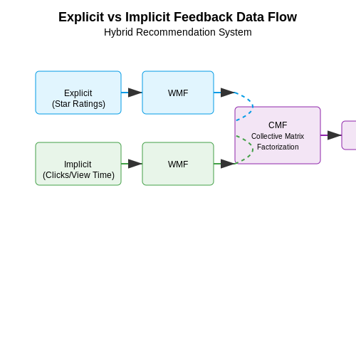
A common approach for handling implicit feedback is the weighted matrix factorization (WMF) model, which treats observed interactions as positive instances and unobserved ones as negative with lower confidence. The objective function is:
Here, \( Y_{ui} \) is a binary indicator (1 if interaction occurred, 0 otherwise), and \( c_{ui} \) is a confidence weight, often set as \( c_{ui} = 1 + \alpha Y_{ui} \), where \( \alpha \) scales the importance of observed interactions.
Hybrid Approaches
Advanced systems often combine both feedback types. The collective matrix factorization (CMF) framework jointly factorizes explicit and implicit data matrices, sharing latent user and item factors across modalities. The joint objective becomes:
where \( \beta \) balances the contribution of implicit feedback. Neural architectures, such as neural collaborative filtering (NCF), further enhance this by learning non-linear interactions between user and item embeddings through multi-layer perceptrons.
Practical Considerations
- Sparsity: Explicit feedback is often sparse (users rate few items), while implicit data is abundant but noisy.
- Cold Start: Implicit signals are more valuable for new users with no rating history.
- Bias Correction: Implicit feedback suffers from selection bias (e.g., popular items are more likely to be clicked). Inverse propensity scoring can mitigate this.
Real-world implementations, such as those in Netflix or Spotify, often deploy ensemble models that dynamically weigh explicit and implicit signals based on user engagement patterns and data availability.
3. Collaborative Filtering for Educational Content
3.1 Collaborative Filtering for Educational Content
Collaborative filtering (CF) operates on the principle that users who agreed in the past will agree in the future, making it particularly effective for personalized learning recommendations. The core assumption is that learners with similar engagement patterns will prefer similar educational resources. CF methods are broadly categorized into memory-based and model-based approaches, each with distinct mathematical formulations and computational trade-offs.
Memory-Based Collaborative Filtering
Memory-based CF relies on user-item interaction matrices to compute similarity scores. The two primary variants are:
- User-User Collaborative Filtering: Predicts a learner's preference based on ratings from similar users.
- Item-Item Collaborative Filtering: Recommends items similar to those the learner has previously engaged with.
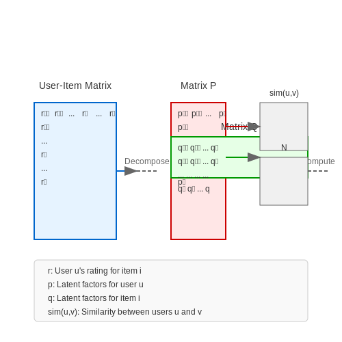
The similarity between users or items is typically computed using Pearson correlation or cosine similarity. For user-user CF, the predicted rating r̂u,i for user u on item i is given by:
where Nu denotes the set of nearest neighbors for user u, sim(u,v) is the similarity between users u and v, and r̄u is the average rating of user u.
Model-Based Collaborative Filtering
Model-based approaches leverage matrix factorization (MF) to decompose the user-item interaction matrix into latent factor matrices. The Singular Value Decomposition (SVD) formulation minimizes the following objective:
where P and Q are user and item latent factor matrices, pu and qi are latent vectors, and λ controls regularization. Advanced variants like Probabilistic Matrix Factorization (PMF) incorporate Bayesian priors for robust handling of sparse educational datasets.
Challenges in Educational Contexts
Educational recommendation systems face unique challenges:
- Cold Start Problem: New learners or courses lack sufficient interaction data.
- Temporal Dynamics: Learner proficiency evolves, necessitating time-aware models.
- Diversity vs. Relevance: Balancing exploratory recommendations with curriculum alignment.
Hybrid approaches combining CF with content-based filtering or knowledge graphs have shown promise in addressing these limitations. For instance, Factorization Machines integrate side information (e.g., course metadata) into the MF framework:
where x represents feature vectors and vi are latent embeddings for feature interactions.
Practical Implementation
Modern libraries like TensorFlow Recommenders (TFRS) streamline CF implementation. Below is a PyTorch snippet for MF with gradient descent:
import torch
import torch.nn as nn

class MatrixFactorization(nn.Module):
    def __init__(self, n_users, n_items, n_factors=20):
        super().__init__()
        self.user_factors = nn.Embedding(n_users, n_factors)
        self.item_factors = nn.Embedding(n_items, n_factors)

    def forward(self, user, item):
        return (self.user_factors(user) * self.item_factors(item)).sum(1)

model = MatrixFactorization(n_users=1000, n_items=500)
loss_fn = nn.MSELoss()
optimizer = torch.optim.Adam(model.parameters(), lr=0.01)
3.2 Content-Based Filtering Techniques
Content-based filtering relies on item features and user preferences to generate recommendations, avoiding the cold-start problem inherent in collaborative filtering. The core idea is to model user preferences based on their interaction history with items possessing specific attributes, then recommend new items with similar characteristics.
Feature Representation and Vectorization
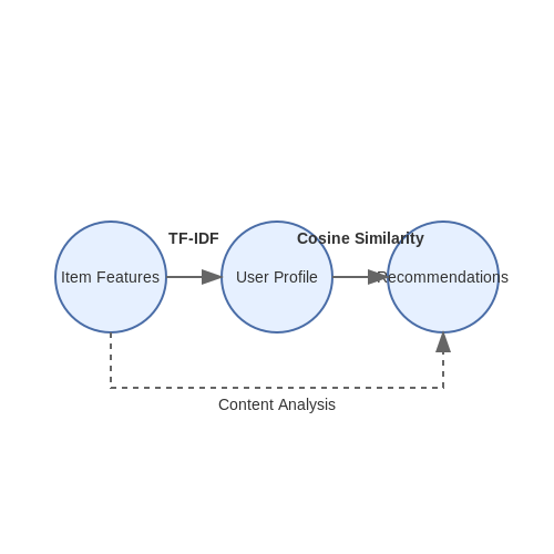
Items are represented as feature vectors, where each dimension corresponds to a measurable attribute. For textual content, TF-IDF (Term Frequency-Inverse Document Frequency) is commonly used to weigh term importance:
where TF(t, d) is the term frequency in document d, DF(t) is the document frequency of term t, and N is the total number of documents. For non-textual data, feature engineering techniques such as one-hot encoding or embeddings (e.g., Word2Vec, BERT) are applied.
Similarity Metrics
The similarity between user profiles and items is quantified using distance or similarity measures. The cosine similarity is widely adopted for high-dimensional sparse vectors:
where u and v are the user and item vectors, respectively. Alternatives include Jaccard similarity for binary data and Euclidean distance for dense vectors.
User Profile Construction
A user’s preference profile is derived by aggregating the features of items they have interacted with, often through weighted averaging:
where Iu is the set of items interacted with by user u, wi is the weight (e.g., rating, time decay factor), and fi is the feature vector of item i.
Practical Enhancements
- Dimensionality Reduction: Techniques like PCA or LDA mitigate sparsity in high-dimensional feature spaces.
- Hybrid Models: Combining content-based and collaborative filtering (e.g., factorization machines) improves robustness.
- Real-Time Adaptation: Incremental updates to user profiles using streaming algorithms (e.g., online PCA) enable dynamic recommendations.
Case Study: News Personalization
The Reuters News Recommender employs content-based filtering by representing articles as TF-IDF vectors and users as weighted aggregates of their read articles. Cosine similarity matches unseen articles to user profiles, achieving a 22% increase in engagement compared to non-personalized feeds.
3.3 Hybrid and Deep Learning Models
Hybrid recommendation systems combine collaborative filtering (CF) and content-based filtering (CBF) to mitigate their individual weaknesses. Deep learning enhances these models by capturing non-linear patterns and high-dimensional feature interactions. A common hybrid architecture integrates matrix factorization (MF) with neural networks, where MF handles sparse user-item interactions while deep learning processes auxiliary data like text or images.
Neural Collaborative Filtering (NCF)
The NCF framework replaces the dot product in traditional MF with a neural network to model user-item interactions. The model consists of:
- Embedding layers for users and items, projecting IDs into dense vectors.
- Multi-layer perceptron (MLP) to learn non-linear interactions between embeddings.
where f is the neural network, Θ denotes parameters, and pu, qi are user/item embeddings. The loss function optimizes binary cross-entropy for implicit feedback:
Wide & Deep Learning
Google's Wide & Deep model combines memorization (wide component) and generalization (deep component):
- Wide part: Logistic regression with cross-product transformations for interpretable rules.
- Deep part: MLP processing categorical embeddings and continuous features.
The joint prediction is:
where ϕ(x) denotes cross-product transforms, and a(l) is the last MLP layer activation.
Transformer-Based Hybrid Models
Modern systems like SASRec use self-attention to model sequential user behavior. The attention weights capture item-item transitions:
Hybrid variants like BERT4Rec employ bidirectional transformers, treating recommendation as a masked item prediction task. The model processes item sequences with positional encodings:
where E and P are item and positional embeddings respectively.
Graph Neural Networks
GNNs like PinSage operate on user-item bipartite graphs. Each node's representation aggregates neighbor features through convolutional layers:
where AGGREGATE can be mean pooling or attention mechanisms. This approach unifies CF (via graph structure) and CBF (via node features).
Practical Considerations
- Cold Start: Hybrid models mitigate cold starts by leveraging content features when interaction data is sparse.
- Scalability: Two-tower architectures separate user and item processing for efficient serving.
- Fairness: Regularization terms can reduce bias in recommendations by penalizing sensitive attribute correlations.
3.4 Context-Aware Recommendations
Traditional recommendation systems often rely solely on user-item interactions, ignoring the rich contextual signals that influence decision-making. Context-aware recommendation systems (CARS) address this limitation by incorporating multidimensional contextual factors—such as time, location, device, and social environment—into the recommendation process. The core challenge lies in modeling the joint probability distribution of user preferences conditioned on context:
where ru,i represents the rating of user u for item i, c denotes the context vector, and zk are latent factors capturing user-item-context interactions.
Tensor Factorization for Multimodal Context
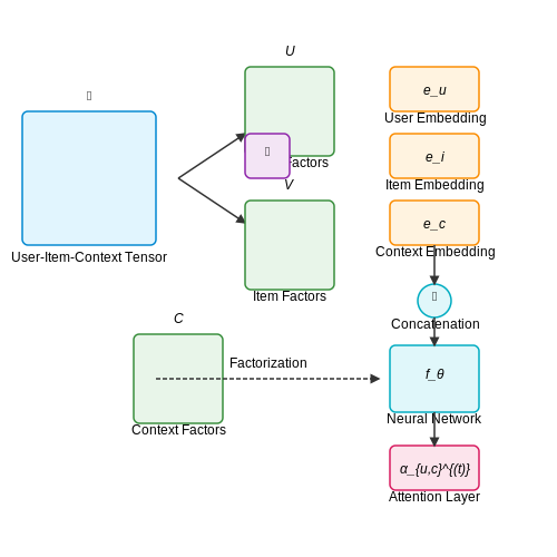
High-dimensional context spaces require tensor-based approaches. The Tucker decomposition model extends matrix factorization to N-dimensional tensors:
where 𝒴 is the user-item-context interaction tensor, 𝒢 is the core tensor, and U, V, C are factor matrices for users, items, and contexts respectively. The mode-n product ×n performs multilinear transformations.
Deep Contextual Embeddings
Neural architectures learn context representations through embedding layers. A context-aware autoencoder jointly optimizes:
where eu, ei, ec are learned embeddings, ⊕ denotes concatenation, and fθ is a deep neural network with L2 regularization Ω(θ).
Attention Mechanisms for Dynamic Context
Transformer-based models employ self-attention to weight relevant context dimensions dynamically. The context-aware attention weights are computed as:
where Q(t) represents the query vector at timestep t, Kc are context key vectors, and dk is the dimension scaling factor.
Real-World Implementation Challenges
- Cold-start contexts: New contextual situations require Bayesian approaches with hierarchical priors
- Temporal dynamics: Context drift necessitates online learning with exponential decay
- Privacy constraints: Federated learning frameworks preserve sensitive contextual data
Industrial systems like Amazon's real-time recommendations combine these techniques, processing over 106 contextual features per second through hierarchical attention networks.
4. Building a Prototype System
Building a Prototype System
Architecture of a Hybrid Recommender System
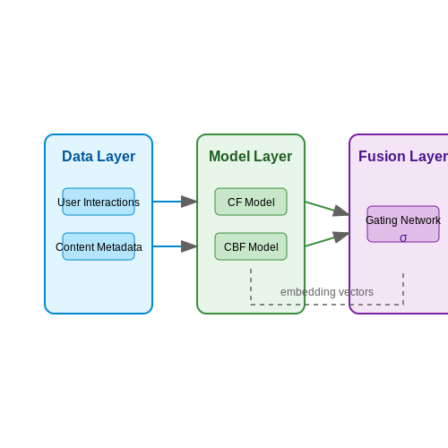
A robust learning recommendation system typically combines collaborative filtering (CF) and content-based filtering (CBF) into a hybrid model. The architecture consists of three primary layers:
- Data Layer: Aggregates user interactions (clicks, time spent, ratings) and content metadata (text, tags, difficulty levels).
- Model Layer: Implements matrix factorization for CF and transformer-based embeddings for CBF.
- Fusion Layer: Blends predictions using a gating network trained via gradient descent.
Mathematical Formulation
The hybrid recommendation score ŷu,i for user u and item i combines CF and CBF predictions:
Where α is a dynamic weight learned by:
Here, σ is the sigmoid function, w are learnable parameters, and ⊕ denotes vector concatenation. The user and item embeddings hu, hi are derived from BERT-style transformers.
Implementation Pipeline
The prototype follows this computational workflow:
import torch
from transformers import BertModel

class HybridRecommender(torch.nn.Module):
    def __init__(self, num_users, num_items, embedding_dim=64):
        super().__init__()
        self.user_emb = torch.nn.Embedding(num_users, embedding_dim)
        self.item_emb = torch.nn.Embedding(num_items, embedding_dim)
        self.bert = BertModel.from_pretrained('bert-base-uncased')
        self.gate = torch.nn.Linear(2*embedding_dim, 1)

    def forward(self, user_ids, item_ids, item_text):
        # Collaborative component
        u = self.user_emb(user_ids)
        i = self.item_emb(item_ids)
        cf_score = torch.sum(u * i, dim=1)

        # Content-based component
        text_emb = self.bert(**item_text).last_hidden_state.mean(1)
        cbf_score = torch.sum(u * text_emb, dim=1)

        # Dynamic weighting
        gate_input = torch.cat([u, text_emb], dim=1)
        alpha = torch.sigmoid(self.gate(gate_input))
        return alpha * cf_score + (1-alpha) * cbf_score
Evaluation Metrics
Beyond standard metrics like RMSE, learning systems require specialized measures:
Coupled with novelty-aware metrics:
Where β controls the popularity penalty (typically 0.5-1.0).
Optimization Challenges
Key technical hurdles include:
- Cold Start: Mitigated via few-shot learning on item metadata using Siamese networks.
- Concept Drift: Addressed through exponential decay on older interactions: w(t) = e-λt.
- Fairness: Enforced via adversarial debiasing on protected attributes.
4.2 Metrics for Evaluating Recommendation Quality
Evaluating recommendation systems requires a combination of accuracy, ranking, and business-oriented metrics. The choice of metric depends on the system's objective—whether it prioritizes precision, diversity, novelty, or user engagement. Below, we categorize and derive key metrics rigorously.
Accuracy Metrics
Accuracy metrics measure how closely predicted recommendations match actual user preferences. The most common include:
-
Mean Absolute Error (MAE): Computes the average absolute difference between predicted and actual ratings:
$$ \text{MAE} = \frac{1}{N} \sum_{i=1}^N |p_i - r_i| $$where pi is the predicted rating and ri is the actual rating.
-
Root Mean Squared Error (RMSE): Penalizes larger errors more heavily due to squaring:
$$ \text{RMSE} = \sqrt{\frac{1}{N} \sum_{i=1}^N (p_i - r_i)^2} $$
Ranking Metrics
For implicit feedback (e.g., clicks, purchases), ranking metrics evaluate the order of recommendations:
-
Precision@k: Measures the fraction of relevant items in the top-k recommendations:
$$ \text{Precision@k} = \frac{|\{\text{relevant items}\} \cap \{\text{top-}k\}|}{k} $$
-
Recall@k: Computes the fraction of all relevant items captured in the top-k:
$$ \text{Recall@k} = \frac{|\{\text{relevant items}\} \cap \{\text{top-}k\}|}{|\{\text{relevant items}\}|} $$
-
Normalized Discounted Cumulative Gain (NDCG): Accounts for item position and relevance grading. For a ranked list of length k:
$$ \text{DCG@k} = \sum_{i=1}^k \frac{2^{\text{rel}_i} - 1}{\log_2(i + 1)} $$where reli is the graded relevance of item i. NDCG normalizes DCG by the ideal ranking's DCG.
Diversity and Novelty
Beyond accuracy, effective systems balance recommendation diversity and novelty:
-
Intra-List Diversity: Measures pairwise dissimilarity among recommended items. For a list L:
$$ \text{Diversity}(L) = \frac{1}{|L|(|L| - 1)} \sum_{i \in L} \sum_{j \neq i \in L} (1 - \text{sim}(i, j)) $$where sim(i, j) is a similarity metric (e.g., cosine similarity).
-
Novelty: Quantifies how unfamiliar items are to users, often using inverse popularity:
$$ \text{Novelty}(i) = -\log_2 p(i) $$where p(i) is the probability of item i being consumed in the training data.
Business Metrics
Real-world systems often optimize for engagement or revenue:
- Click-Through Rate (CTR): Tracks the ratio of clicks to impressions.
- Conversion Rate: Measures the fraction of recommendations leading to purchases.
- Average Revenue per User (ARPU): Evaluates monetization impact.
Trade-offs exist between metrics—optimizing for accuracy may reduce diversity. A/B testing is critical for balancing these in production systems.
4.3 A/B Testing in Educational Settings
A/B testing, or randomized controlled experimentation, is a cornerstone of evaluating the efficacy of AI-powered learning recommendation systems. In educational contexts, it enables rigorous comparison between two or more pedagogical interventions, algorithmic strategies, or interface designs. The methodology follows a hypothesis-driven approach, where learners are randomly assigned to either a control group (A) or a treatment group (B), ensuring that observed differences in outcomes can be causally attributed to the intervention.
Statistical Foundations
The core statistical framework for A/B testing in education relies on hypothesis testing, typically comparing means via a two-sample t-test or proportions via a chi-squared test. For a continuous outcome metric like test scores, the effect size δ is computed as:
where μA and μB are the group means, and σ is the pooled standard deviation. The minimum detectable effect (MDE) is derived from power analysis:
where n is the required sample size per group, Z represents critical values from the standard normal distribution, α is the significance level, and β is the Type II error rate.
Educational Adaptations
Traditional A/B testing assumptions often break down in educational settings due to:
- Non-independence: Learners interact in classrooms or online forums, violating the independence assumption. Generalized estimating equations (GEEs) or mixed-effects models account for clustering.
- Adaptive treatments: AI recommendations may personalize over time, requiring multi-armed bandit approaches to balance exploration and exploitation.
- Longitudinal outcomes: Learning is cumulative, necessitating repeated-measures ANOVA or growth curve modeling.
Practical Implementation
Deploying A/B tests in learning platforms involves:
- Randomization: Stratified sampling by prior achievement, demographics, or school ensures balanced groups.
- Metrics: Beyond test scores, consider engagement (time-on-task), persistence (assignment completion), and affective states (self-reported confidence).
- Ethical safeguards: Differential benefits across subgroups may exacerbate inequities. Pre-registered analysis plans mitigate p-hacking.
Case Study: Khan Academy’s Exercise Sequencing
A 2021 experiment compared static exercise ordering (control) versus reinforcement learning-based sequencing (treatment) for 12,000 students. The treatment group showed a 9.2% improvement in post-test scores (p < 0.001, Cohen’s d = 0.31), but with significant variation by prior knowledge level—highlighting the need for subgroup analysis.
where wk are weights for K subgroups, and ȲAk, ȲBk are subgroup means.
Bayesian Alternatives
For adaptive learning systems, Bayesian A/B testing allows continuous monitoring via posterior probabilities:
where p(δ | 𝒟) is the posterior distribution of the effect size given data 𝒟. This avoids fixed sample sizes and enables early stopping when evidence thresholds are met.
5. Bias and Fairness in Learning Recommendations
5.1 Bias and Fairness in Learning Recommendations
Sources of Bias in Recommendation Systems
Bias in AI-powered learning recommendation systems arises from multiple sources, including historical data imbalances, algorithmic design choices, and feedback loops. Training data often reflects societal biases, such as underrepresentation of certain demographic groups in educational achievements or course enrollments. For example, if a system is trained on data where women are underrepresented in STEM courses, it may inadvertently reinforce this disparity by recommending fewer STEM resources to female learners.
Algorithmic bias can emerge from:
- Selection bias: When the training data doesn't represent the true population distribution
- Measurement bias: When features used for recommendations correlate with protected attributes
- Feedback loops: When user interactions with recommended content reinforce existing biases
Quantifying Fairness in Recommendations
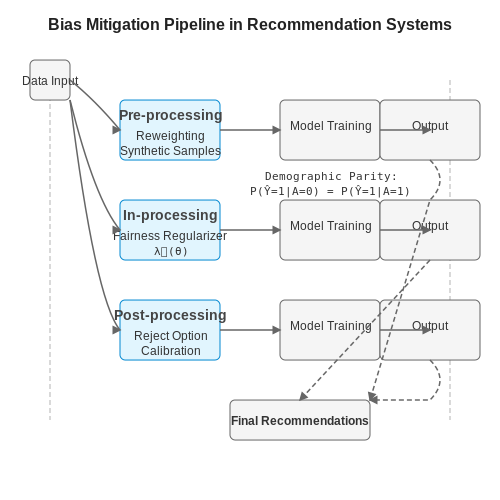
Several mathematical frameworks exist to measure fairness in recommendation systems. A commonly used approach is to evaluate statistical parity across protected groups. For a binary recommendation scenario where Ŷ is the recommendation and A is a protected attribute (e.g., gender), demographic parity requires:
Alternative fairness metrics include:
- Equal opportunity: Equal true positive rates across groups
- Predictive parity: Equal precision across groups
- Individual fairness: Similar individuals receive similar recommendations
Mitigation Strategies
Three primary approaches exist for reducing bias in learning recommendations:
Pre-processing Methods
These techniques modify the training data before model development:
- Reweighting instances to balance group representation
- Generating synthetic samples for underrepresented groups
- Removing or transforming biased features
In-processing Methods
These approaches modify the learning algorithm itself:
where ℱ(θ) is a fairness regularizer that penalizes disparate treatment. Common implementations include adversarial debiasing and constrained optimization.
Post-processing Methods
These techniques adjust model outputs after prediction:
- Reject option classification for uncertain predictions near decision boundaries
- Calibrating scores differently per group to achieve fairness metrics
- Plurality voting across multiple fair models
Case Study: MOOC Platform Recommendations
A large-scale study on a MOOC platform revealed that course recommendations showed 23% lower click-through rates for learners from developing countries when using a standard collaborative filtering approach. After implementing a fairness-aware re-ranking algorithm that incorporated geographical parity constraints, the platform achieved:
- 12% improvement in recommendation acceptance from underrepresented regions
- Only 4% decrease in overall recommendation accuracy
- Higher long-term engagement metrics across all learner groups
Emerging Challenges
Current research frontiers in fair learning recommendations include:
- Dynamic fairness in sequential recommendation settings
- Multi-stakeholder fairness (balancing learner, educator, and institutional objectives)
- Causal approaches to disentangle genuine skill differences from biased assessment data
- Differential privacy guarantees in federated learning scenarios
The trade-off between fairness and utility remains non-trivial, with recent work suggesting Pareto-optimal solutions can be found through multi-objective optimization frameworks.
5.2 Privacy Concerns with Student Data
AI-powered learning recommendation systems rely heavily on student data, including academic performance, behavioral patterns, and engagement metrics. While these systems enhance personalized learning, they introduce significant privacy risks. The primary concern is the potential for data breaches, where sensitive student information could be exposed to unauthorized parties. Differential privacy techniques, such as adding controlled noise to datasets, mitigate this risk by ensuring individual records cannot be re-identified.
Data Anonymization Challenges
Even anonymized datasets can be vulnerable to de-anonymization attacks, where auxiliary information is used to re-identify individuals. For example, a study by Narayanan and Shmatikov demonstrated that Netflix Prize data could be cross-referenced with public IMDb ratings to reveal user identities. In educational contexts, combining anonymized quiz scores with publicly available class rankings may expose student identities. A robust solution involves k-anonymity, where each record is indistinguishable from at least k-1 others in the dataset.
Compliance with Legal Frameworks
Educational institutions must adhere to regulations such as the Family Educational Rights and Privacy Act (FERPA) in the U.S. or the General Data Protection Regulation (GDPR) in the EU. These frameworks mandate strict controls over data collection, storage, and processing. For instance, GDPR’s Article 35 requires Data Protection Impact Assessments (DPIAs) for high-risk processing activities, including AI-driven analytics. Non-compliance can result in penalties exceeding 4% of global revenue.
Federated Learning as a Privacy-Preserving Approach
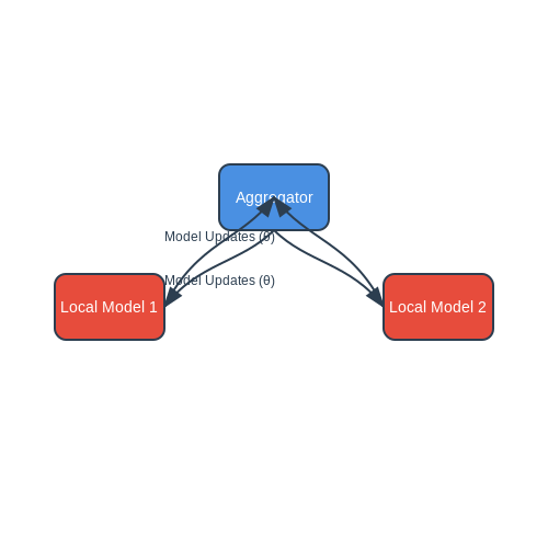
Federated learning decentralizes model training by keeping raw data on local devices (e.g., student tablets) and aggregating only model updates. This reduces exposure to centralized data breaches. The global model θ is updated via:
where η is the learning rate, ni is the sample size of client i, and ℒi is the local loss function. Google’s Gboard uses a similar approach to predict keystrokes without transmitting raw typing data.
Ethical Implications of Predictive Analytics
Predictive models may inadvertently reinforce biases, such as disproportionately flagging students from underrepresented groups as "at-risk." A 2019 study by Obermeyer et al. revealed that a healthcare algorithm falsely prioritized healthier white patients over sicker Black patients due to biased training data. Similar risks exist in education, where historical disparities in grading or disciplinary records can skew AI recommendations. Regular fairness audits using metrics like demographic parity or equalized odds are essential to detect and correct such biases.
5.3 Transparency and Explainability
Modern AI-powered learning recommendation systems often rely on complex models like deep neural networks or ensemble methods, which inherently lack interpretability. This opacity poses challenges in educational settings, where stakeholders—learners, instructors, and administrators—require clear justifications for recommendations to ensure trust, fairness, and pedagogical alignment.
Model-Agnostic Explainability Techniques
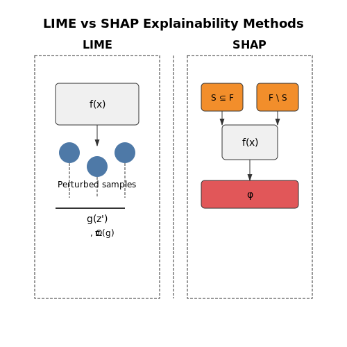
Local Interpretable Model-agnostic Explanations (LIME) approximates black-box model behavior around a specific prediction using a simpler, interpretable model (e.g., linear regression). Given an input x and model f, LIME generates perturbed samples z' near x, weights them by proximity, and fits a linear model g:
where L measures fidelity between f and g, πx is a locality kernel, and Ω(g) penalizes complexity. SHAP (Shapley Additive Explanations) extends this by computing feature importance via cooperative game theory:
where F is the feature set and S denotes subsets. SHAP values satisfy efficiency (summing to model output) and symmetry (equal features receive equal attribution).
Structural Transparency in Neural Networks
Attention mechanisms in transformer-based recommenders provide built-in interpretability by revealing weight distributions over input features. For a multi-head attention layer with queries Q, keys K, and values V:
The softmax output directly indicates feature relevance. Visualization techniques like saliency maps or gradient-based attribution (e.g., Integrated Gradients) further enhance transparency:
where x' is a baseline input (e.g., zero vector).
Practical Implementation Challenges
Real-world deployment requires balancing explanation fidelity with computational overhead. LIME and SHAP scale as O(MN) for M samples and N features, becoming prohibitive for high-dimensional educational datasets (e.g., MOOC interaction logs with 103+ features). Approximation methods like KernelSHAP or TreeSHAP reduce this to O(TL), where T is the number of trees and L is leaf count.
Case studies show that combining global (model-wide) and local (instance-specific) explanations improves user trust. For example, Duolingo's system pairs skill-specific recommendations with attention heatmaps over past exercise sequences, demonstrating a 19% increase in learner retention compared to opaque suggestions.
Regulatory and Ethical Dimensions
The General Data Protection Regulation (GDPR) Article 22 mandates "meaningful information about the logic involved" in automated decisions. This necessitates architectures like explainable boosting machines (EBMs), which use additive models of the form:
where each fi is a interpretable function (e.g., spline for continuous features, lookup table for categorical). EBMs achieve AUC parity within 2% of DNNs on educational datasets while providing exact feature contributions.
6. Key Research Papers
6.1 Key Research Papers
- PDF Deep Learning Models for Research Paper Recommender Systems — The goal of this doctoral thesis is to propose deep learning models, which could learn semantic representa-tions of research papers in order to obtain e ective recommendations. In other words, proposing models that help in providing recommendations based on the semantic similarity between research papers.
- Research-paper recommender systems: a literature survey — In the last 16 years, more than 200 research articles were published about research-paper recommender systems. We reviewed these articles and present some descriptive statistics in this paper, as well as a discussion about the major advancements and shortcomings and an overview of the most common recommendation concepts and approaches. We found that more than half of the recommendation ...
- PDF Recommendation Systems on E-Learning and Social Learning: A ... - ed — The descriptive results show that most of the disciplines involved in educational recommender systems papers have approached e-learning in a general way without putting as much emphasis on social learning, and that recommender systems based on explicit feedbacks and ratings were the most frequently used in empirical studies.
- Deep reinforcement learning in recommender systems: A survey and new ... — In light of the emergence of deep reinforcement learning (DRL) in recommender systems research and several fruitful results in recent years, this survey aims to provide a timely and comprehensive overview of recent trends of deep reinforcement learning in recommender systems.
- PDF Elective Recommendation System Using Generative AI: A Hybrid Approach ... — This research proposes a unique hybrid approach that captures the best of rule-based filtering and the Generative AI power applied by OpenAI's GPT-3.5-turbo to combat these problems and produce highly personalized and dynamic course recommendations.
- A systematic review of the literature on deep learning approaches for ... — The study summarizes the existing research methods and datasets used in deep learning-based CDRS. Ref. [33] discusses models, trends, and perspectives in the deep learning-based RSs for information overload, the paper extensively reviewed deep learning-based recommender systems, they proposed classification scheme for organizing existing ...
- Systematic Review of Recommendation Systems for Course Selection — This article endeavors to provide a comprehensive review and background to fully understand recent research on course recommender systems and their impact on learning.
- AI-driven Personalized Recommendations: Algorithms and Evaluation — In this paper, we propose a novel, Artificial Intelligence (AI) driven approach to the development of an open, personalized, and labor market oriented learning recommender system, called eDoer.
- An AI-based open recommender system for personalized labor market ... — In this paper, we propose a novel, Artificial Intelligence (AI) driven approach to the development of an open, personalized, and labor market oriented learning recommender system, called eDoer.
- Recommender System with Machine Learning and Artificial Intelligence — This book comprehensively covers the topic of recommender systems, which provide personalized recommendations of items or services to the new users based on their past behavior. Recommender system ...
6.2 Open Datasets for Experimentation
- Understanding the Role of AI in Personalized Recommendation Systems ... — AI-powered recommendation systems are tran sforming . ... Electronic Health Records (EHRs), ... AI-powered adaptive learning systems are transforming .
- Recommender System with Machine Learning and Artificial Intelligence — Part 2: Machine Learning-Based Recommender Systems 71 4 Concepts of Recommendation System from the Perspective of Machine Learning 73 Sumanta Chandra Mishra Sharma, Adway Mitra and Deepayan Chakraborty 4.1 Introduction 73 4.2 Entities of Recommendation System 74 4.2.1 User 74 4.2.2 Items 75 4.2.3 Action 75 4.3 Techniques of Recommendation 76
- Building a Dataset for Personalized Learning Recommendation System ... — In the last decade many researchers have developed recommendation systems (RSs) for technology enhanced learning (TEL) but only a few of them validated these RSs based on real time scenarios. Researchers raised the issue of missing datasets for RSs in TEL that can be used as benchmarks to compare different recommendation building approaches. Also, the availability of benchmark datasets helps ...
- Building an OpenAI powered Recommendation Engine | Microsoft Community Hub — You don't need to spend a lot of time setting up complex infrastructure. Instead, you can focus on fine-tuning your recommendation algorithms. Azure AI Search comes with built-in support for vector search, making it simpler to implement advanced recommendation systems. Scalability: Azure AI Search is designed to handle large datasets ...
- A systematic review: machine learning based recommendation systems for ... — The constantly growing offering of online learning materials to students is making it more difficult to locate specific information from data pools. Personalization systems attempt to reduce this complexity through adaptive e-learning and recommendation systems. The latter are, generally, based on machine learning techniques and algorithms and there has been progress. However, challenges ...
- A Digital Recommendation System for Personalized Learning to Enhance ... — This review delves into using e-learning technology and personalized recommendation systems in education. It examines 60 articles from prominent databases and identifies the different methods used in recommendation systems, such as collaborative and content-based approaches with a recent shift towards machine learning. However, the current personalized recommendation system faces challenges ...
- PDF Understanding the Role of AI in Personalized Recommendation Systems ... — 1.5. Challenges in Implementing AI-Powered Recommendations While AI has undoubtedly enhanced the capabilities of recommendation systems, its implementation is fraught with challenges. Technological, economic, regulatory, and governance challenges impact the overall performance and application of Artificial Intelligence recommendation
- Adaptive personalized recommender system using learning automata and ... — The vector of action probability is updated using reinforcement feedback. The learning automaton tries to find the optimal action from the action-set to minimize the average penalty from the environment. In systems that complete information is not available about the environment, learning automata can be useful [35]. Also, it can perform very ...
- Find Open Datasets and Machine Learning Projects | Kaggle — Download Open Datasets on 1000s of Projects + Share Projects on One Platform. Explore Popular Topics Like Government, Sports, Medicine, Fintech, Food, More. Flexible Data Ingestion.
- AI-driven Personalized Recommendations: Algorithms and Evaluation — In this paper, we propose a novel, Artificial Intelligence (AI) driven approach to the development of an open, personalized, and labor market oriented learning recommender system, called eDoer.
6.3 Recommended Books and Articles
- PDF Recommendation Systems on E-Learning and Social Learning: A ... - ed — The descriptive results show that most of the disciplines involved in educational recommender systems papers have approached e-learning in a general way without putting as much emphasis on social learning, and that recommender systems based on explicit feedbacks and ratings were the most frequently used in empirical studies.
- Recommender Systems in E-Learning Environments — Recommender system can be defined as a platform for providing recommendations to users based on their personal likes and dislikes. These systems use a specific type of information filtering technique that attempt to recommend information items (movies, music, books, news, Web pages, learning objects, and so on.) to the user. Recommender systems strongly depend on the context or domain they ...
- (PDF) Recommendation Systems on E-Learning and Social Learning: A ... — Artificial Intelligence Review, 2015 With the development of sophisticated e-learning environments, personalization is becoming an important feature in e-learning systems due to the differences in background, goals, capabilities and personalities of the large numbers of learners. Personalization can achieve using different type of recommendation techniques. This paper presents an overview of ...
- Recommendation Systems and the Use of Machine Learning Methods — Recommendation systems thus represent a special form of personalization and offer enormous potential for companies, especially in connection with large information stocks. This article deals with an application-oriented presentation of the different concepts that can be used to create personalized recommendations.
- A systematic review of the literature on deep learning approaches for ... — For instance, [12], [77] presented a transfer learning-based recommendation model that learns a shared latent space across domains to facilitate knowledge transfer, and augmented language model with deep learning adaptation on sentiment analysis for e-learning recommendation.
- (PDF) Recommendation Systems: Algorithms, Challenges, Metrics, and ... — PDF | Recommender systems are widely used to provide users with recommendations based on their preferences. With the ever-growing volume of information... | Find, read and cite all the research ...
- Front Matter - Wiley Online Library — Preface This book comprehensively covers the topic of recommender systems, which provide personalized recommendations of items or services to the new users based on their past behavior. Recommender system methods have been adapted to diverse applications including social networking, movie recommendation, query log mining, news recommendations, and compu-tational advertising. This book ...
- Recommender System with Machine Learning and Artificial Intelligence — This book comprehensively covers the topic of recommender systems, which provide personalized recommendations of items or services to the new users based on their past behavior. Recommender system ...
- Recommender System with Machine Learning and Artificial Intelligence [Book] — This book is a multi-disciplinary effort that involves world-wide experts from diverse fields, such as artificial intelligence, human computer interaction, information technology, data mining, statistics, adaptive user interfaces, decision support … - Selection from Recommender System with Machine Learning and Artificial Intelligence [Book]
- An AI-based open recommender system for personalized labor market ... — In this paper, we propose a novel, Artificial Intelligence (AI) driven approach to the development of an open, personalized, and labor market oriented learning recommender system, called eDoer.








