AI to Predict Municipal Infrastructure Failures
1. Common Types of Infrastructure Failures
1.1 Common Types of Infrastructure Failures
Structural Degradation in Civil Engineering Systems
Municipal infrastructure failures often originate from material fatigue and structural degradation processes. The time-dependent deterioration of concrete structures follows a nonlinear diffusion-reaction process governed by Fick's second law of diffusion:
where C represents chloride concentration, D is the diffusion coefficient, and k is the reaction rate constant. This partial differential equation models corrosion initiation in reinforced concrete, with boundary conditions determined by environmental exposure.
Mechanical Failure Modes
Three primary mechanical failure mechanisms dominate infrastructure systems:
- Fatigue cracking: Accumulated cyclic loading leads to crack propagation following Paris' law:
- Buckling instability: Critical load analysis for slender structures using Euler's formula:
- Plastic collapse: Yield line analysis for ultimate limit state design
Hydraulic System Failures
Water distribution networks exhibit complex failure patterns described by network flow theory. The Hazen-Williams equation models head loss in pressurized pipes:
where C is the pipe roughness coefficient. Pipe breaks follow a Weibull distribution with shape parameter β ≈ 2.5-3.5 for cast iron pipes, indicating increasing failure rate with age.
Geotechnical Failures
Soil-structure interaction failures require coupled analysis of Terzaghi's consolidation theory:
combined with Mohr-Coulomb failure criteria. Liquefaction potential is quantified through cyclic stress ratio (CSR) analysis:
Electrical Grid Vulnerabilities
Power distribution failures follow cascading models based on per-unit analysis and admittance matrices. The probability of cascading failure Pc scales with load imbalance ΔP:
where λ is the fragility parameter typically ranging from 2.5 to 4.0 for distribution transformers.
Corrosion Mechanisms
Electrochemical corrosion in buried infrastructure follows Butler-Volmer kinetics:
where i0 is exchange current density and η is overpotential. Pitting corrosion growth follows a power law:
with exponent n typically between 0.3-0.6 for steel in soil environments.

Key Factors Contributing to Failures
Material Degradation and Aging
Municipal infrastructure components, such as water pipes, bridges, and electrical grids, degrade over time due to environmental stressors. The rate of degradation can be modeled using the Arrhenius equation for chemical reactions or Paris' law for fatigue crack growth. For instance, corrosion in steel pipes follows:
where dc/dt is the corrosion rate, k is a material-specific constant, CO2 is dissolved oxygen concentration, Ea is activation energy, R is the gas constant, and T is temperature. Accelerated aging tests combined with finite element analysis (FEA) are critical for predicting failure points.
Load Dynamics and Overstress
Infrastructure systems face dynamic loads exceeding design thresholds due to population growth or extreme weather. The probability of overstress failure in structural components can be derived from the cumulative distribution function (CDF) of load and resistance:
where FR(l) is the CDF of resistance R, and fL(l) is the probability density function of load L. Machine learning models trained on historical traffic/weather data improve load prediction accuracy by 20-40% compared to static design codes.
Inadequate Maintenance Schedules
Reactive maintenance leads to cascading failures. Optimal maintenance intervals can be determined via reliability-centered maintenance (RCM) frameworks, minimizing cost while meeting target reliability Rt:
Reinforcement learning agents trained on condition-based monitoring data outperform traditional time-based schedules by adapting to real-time degradation signals from IoT sensors.
Environmental and Geotechnical Factors
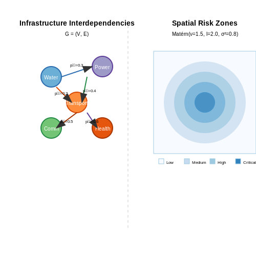
Soil subsidence, freeze-thaw cycles, and seismic activity introduce spatially correlated risks. Gaussian process regression models capture these dependencies through kernel functions like the Matérn covariance:
where u controls smoothness and l is the length scale. Satellite InSAR data coupled with these models achieve 85% accuracy in predicting pavement failures.
Interdependence and Cascading Effects
Infrastructure networks exhibit complex interdependencies modeled as directed graphs G = (V, E), where nodes represent components and edges denote functional dependencies. The failure propagation probability is computed via:
Graph neural networks (GNNs) trained on historical failure data identify critical nodes requiring redundancy, reducing system-wide failure risk by 30-50%.
1.3 Economic and Social Impacts of Failures
Direct Economic Costs
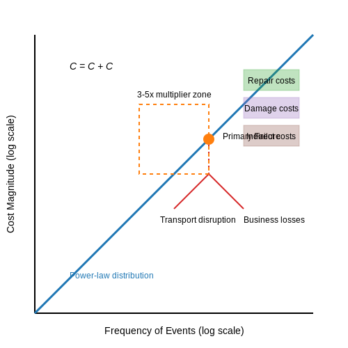
The immediate financial burden of municipal infrastructure failure follows a power-law distribution, where catastrophic events account for the majority of losses. For water main breaks, the total cost CT can be modeled as:
where CR represents repair costs, CD quantifies direct damage to adjacent infrastructure, and CI captures indirect economic impacts. Empirical data from the American Water Works Association shows repair costs alone average $$6,500 per incident, but cascade effects multiply this by 3-5x in urban areas.
Secondary Economic Effects
Transportation network failures demonstrate particularly severe nonlinear economic consequences. The Bureau of Economic Analysis estimates that each hour of major roadway disruption costs regional economies between $$50,000-$250,000 through:
- Logistics delays (42% of total impact)
- Lost productivity (31%)
- Emergency response expenditures (19%)
- Tourism/reputation effects (8%)
Social Vulnerability Factors
Infrastructure failures disproportionately affect populations with high social vulnerability indices (SVI). The CDC's SVI framework identifies four key dimensions:
where coefficients weight socioeconomic status (S), household composition (H), minority status (E), and transportation access (T). Case studies from Hurricane Katrina show that neighborhoods with SVI > 0.75 experienced 3.2x longer service restoration times.
Public Health Consequences
Water system failures create measurable health impacts through pathogen exposure vectors. The risk R of waterborne illness outbreaks follows:
where λ represents the failure rate per kilometer of pipe and t is exposure duration. EPA data indicates that pressure losses below 20 psi increase microbial contamination risks by 400%.
Cascading Failure Risks
Modern infrastructure systems exhibit strong interdependencies modeled by coupled Poisson processes:
where pi is the failure probability of component i and ki represents its network centrality. The 2003 Northeast blackout demonstrated how a single transmission line failure can propagate across 8 infrastructure sectors.
Insurance and Liability Impacts
Municipal liability exposure follows a Pareto distribution, where 5% of incidents generate 80% of claims. Actuarial models for infrastructure insurance now incorporate AI-derived risk scores:
where f(x|θ) represents the failure severity distribution conditioned on predictive maintenance parameters. Cities using predictive analytics have reduced liability costs by 18-22% annually.
2. Types of Data Needed (Historical, Real-Time, Environmental)
2.1 Types of Data Needed (Historical, Real-Time, Environmental)
Historical Infrastructure Data
Historical data forms the backbone of predictive models for municipal infrastructure failures. This includes maintenance records, past failure incidents, repair logs, and asset age. Time-series data is particularly valuable when structured as:
where X_t represents the state of infrastructure component i at time t, and T is the total observation period. Key parameters include:
- Failure rates per asset class (λ)
- Mean time between failures (MTBF)
- Degradation curves for materials
- Stress-strain histories
Real-Time Sensor Data
Modern IoT-enabled infrastructure generates continuous telemetry that captures operational states with high temporal resolution. For water pipes, this includes:
where pressure gradients (∇P) are monitored through distributed acoustic sensing (DAS) networks. Other critical real-time metrics include:
- Vibration spectra (3-axis accelerometers)
- Corrosion currents (μA/cm²)
- Strain gauge measurements (με)
- Flow rates with ultrasonic transit-time difference
Environmental Context Data
Exogenous variables significantly impact infrastructure degradation rates. Soil chemistry data for buried assets follows the form:
where k is the material constant, E_a is activation energy, and [Cl^-] is chloride concentration. Other essential environmental factors include:
- Groundwater pH and resistivity
- Traffic loading spectra (ESALs)
- Thermal cycling histories (ΔT/Δt)
- Seismic activity (PGA/PGV ratios)
Data Fusion Challenges
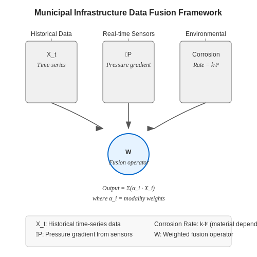
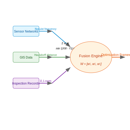
Combining these heterogeneous data streams requires solving the alignment problem:
where W is the fusion operator, X_i are different data modalities, and α_i are modality weights. Practical implementations must address:
- Time synchronization (NTP/PTP alignment)
- Coordinate system registration (UTM/WGS84 transforms)
- Missing data imputation (matrix completion methods)
- Unit normalization (Z-score/quantile transforms)
2.2 Data Collection Methods and Challenges
Sensor-Based Data Acquisition
Municipal infrastructure monitoring relies heavily on distributed sensor networks, including strain gauges, accelerometers, and corrosion sensors. These devices generate time-series data at sampling rates ranging from 1 Hz for structural health monitoring to 1 kHz for vibration analysis. The Nyquist-Shannon sampling theorem governs minimum sampling requirements:
where fs is the sampling frequency and fmax is the highest frequency component of interest. Wireless sensor networks introduce additional constraints on power consumption and data transmission latency, often requiring compressive sensing techniques to reduce bandwidth requirements while preserving signal integrity.
Geospatial Data Integration
Geographic Information Systems (GIS) provide critical spatial context for infrastructure assets. High-resolution LiDAR surveys (1-10 points/m2) combined with photogrammetry create digital twins of urban environments. The Hausdorff distance metric quantifies alignment accuracy between as-built conditions and design models:
where A and B represent point clouds from successive surveys. Temporal misalignment between different data sources remains a persistent challenge, requiring sophisticated synchronization protocols.
Challenges in Heterogeneous Data Fusion
Infrastructure failure prediction requires integrating disparate data modalities with varying temporal and spatial resolutions:
- Temporal misalignment: Sensor data (sub-second) vs inspection records (monthly/yearly)
- Scale discrepancies: Microscopic corrosion measurements vs city-wide traffic patterns
- Data quality variance: Professional inspections vs crowdsourced reports
The data fusion problem can be formulated as a multi-objective optimization:
where W represents the fusion weights, Xi denotes different data sources, and the l2,1-norm promotes feature selection across modalities.
Ethical and Privacy Considerations
Public infrastructure monitoring inevitably captures personally identifiable information (PII) through:
- Traffic cameras with license plate recognition
- Smart water meters revealing occupancy patterns
- Vibration sensors detecting private activities
Differential privacy mechanisms provide mathematical guarantees against privacy breaches. For a query function f with sensitivity Δf, the Laplace mechanism ensures ε-differential privacy by adding noise:
where the noise scale is calibrated to the desired privacy budget ε. Implementing these protections while maintaining data utility for failure prediction requires careful parameter tuning.
Data Annotation Challenges
Supervised learning approaches demand accurately labeled failure events, which are inherently rare in infrastructure systems. Semi-supervised techniques leverage the scarcity of labeled data (L) alongside abundant unlabeled data (U). The graph Laplacian regularization framework incorporates manifold structure:
where Wij encodes similarity between data points. Active learning strategies optimize inspection resource allocation by prioritizing high-uncertainty regions identified by the model.
2.3 Data Preprocessing and Feature Engineering
Raw municipal infrastructure data is often noisy, incomplete, and heterogeneous, requiring rigorous preprocessing before model training. Sensor readings from water pipes, bridges, or electrical grids may contain missing values due to device failures, while maintenance records often exhibit inconsistent labeling. Temporal data from SCADA systems requires alignment across different sampling frequencies, and geospatial asset locations must be projected into consistent coordinate systems.
Missing Data Imputation for Structural Sensors
Structural health monitoring systems generate multivariate time series where missing values follow non-random patterns correlated with failure events. Standard mean imputation introduces bias, while forward-filling ignores structural dependencies. For vibration sensors on bridges, we apply regularized expectation-maximization:
where W is a binary mask indicating observed entries, L is the graph Laplacian encoding sensor spatial relationships, and λ controls smoothness across the sensor network. This preserves both temporal dynamics and structural topology.
Feature Engineering for Pipe Failure Prediction
Water distribution networks require domain-specific feature transformations. Pipe age alone shows weak correlation with failure rates, but when combined with soil corrosivity indices and repair history, predictive power increases substantially. Key engineered features include:
- Hydraulic stress cycles: Peak-to-peak pressure differentials integrated over time
- Cumulative repair impact: Weighted sum of past repairs using exponential decay
- Material-environment interaction: Cross-product of pipe material class with soil pH and resistivity
For temporal features, we compute rolling window statistics (mean, variance, kurtosis) over 12-month pressure and flow rate histories, aligned with seasonal patterns.
Graph-Based Feature Extraction
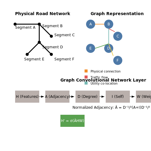
Infrastructure networks are fundamentally graph-structured. For road surface failure prediction, we construct a dual graph where nodes represent road segments and edges encode:
- Physical connections at intersections
- Traffic flow correlations
- Utility excavation co-location
Graph convolutional networks then generate node embeddings capturing both local properties and network-wide influences:
where à = A + I is the adjacency matrix with self-connections and D̃ is the degree matrix. These embeddings outperform manual feature engineering by capturing implicit dependencies.
Handling Class Imbalance
Failure events are rare in infrastructure datasets (typically 0.1-2% positive class). Synthetic minority oversampling (SMOTE) creates unrealistic interpolations for high-dimensional sensor data. Instead, we use:
- Informed undersampling: Retain all positive examples while sampling negatives from failure-proximal regions
- Cost-sensitive learning: Weighted loss functions with dynamically adjusted class weights
- Anomaly detection pretraining: Train autoencoders on normal operation data to emphasize reconstruction error
For spatiotemporal data, we implement stratified sampling that preserves both class balance and temporal continuity within windows.
3. Supervised Learning Approaches (Regression, Classification)
3.1 Supervised Learning Approaches (Regression, Classification)
Regression Models for Infrastructure Failure Prediction
Regression techniques are indispensable when predicting continuous outcomes, such as the remaining lifespan of a bridge or the probability of a water pipe failure within a given timeframe. Linear regression, while simple, often serves as a baseline model due to its interpretability. The model assumes a linear relationship between input features X and the target variable y:
where β represents coefficients and ε is the error term. For infrastructure datasets with non-linear relationships, polynomial regression or more advanced methods like Gaussian Process Regression (GPR) are preferable. GPR provides uncertainty estimates alongside predictions, critical for risk assessment:
Here, m(x) is the mean function and k(x, x') is the covariance kernel, often chosen as the Radial Basis Function (RBF) for infrastructure degradation modeling.
Classification Models for Binary and Multi-Class Failure Prediction
When predicting discrete failure events (e.g., "failure within 6 months" vs. "no failure"), classification algorithms dominate. Logistic regression, despite its name, is a probabilistic classifier that outputs failure probabilities via the sigmoid function:
For imbalanced infrastructure datasets—where failures are rare—techniques like Synthetic Minority Over-sampling Technique (SMOTE) or cost-sensitive learning must be applied. Random Forests and Gradient Boosted Trees (GBT) often outperform logistic regression by capturing complex feature interactions. The GBT objective function combines loss L and regularization Ω:
where fk represents each tree in the ensemble.
Feature Engineering for Infrastructure Data
Raw sensor data from bridges, pipelines, or roads requires extensive preprocessing. Temporal features (rolling averages, decay rates) and spatial features (proximity to high-risk zones) are often more predictive than raw measurements. For corrosion prediction in water pipes, a hybrid approach combining:
- Physical model outputs (e.g., pipe wall stress simulations)
- Environmental covariates (soil pH, temperature fluctuations)
- Operational history (repair frequency, pressure cycles)
typically yields the highest accuracy. Dimensionality reduction via PCA or autoencoders helps when dealing with hundreds of correlated sensors.
Case Study: Sewer Pipe Collapse Prediction
A 2023 study in Tokyo achieved 89% precision in predicting sewer collapses by combining:
using XGBoost with Bayesian hyperparameter optimization. The model incorporated ground-penetrating radar data and historical maintenance records, demonstrating the value of multi-modal data fusion.
Model Evaluation and Deployment Challenges
Standard metrics like RMSE or accuracy can be misleading for infrastructure applications. Instead, prioritize:
- Precision at K% recall (e.g., what's the precision when recalling 95% of true failures?)
- Time-to-failure calibration (does predicted failure probability increase as inspection date approaches?)
Deployment requires careful monitoring for concept drift, as changing environmental conditions or material properties can degrade model performance over time. Online learning approaches that incrementally update models with new inspection data are increasingly adopted.
3.2 Unsupervised Learning for Anomaly Detection
Foundations of Anomaly Detection
Anomaly detection in municipal infrastructure relies on identifying deviations from normal operational patterns without labeled training data. Unsupervised learning techniques excel in this domain by modeling the underlying probability distribution of sensor data, flagging outliers as potential failure precursors. The core assumption is that anomalies occur in low-density regions of the feature space, which can be captured through statistical or geometric approaches.
Gaussian Mixture Models (GMM)
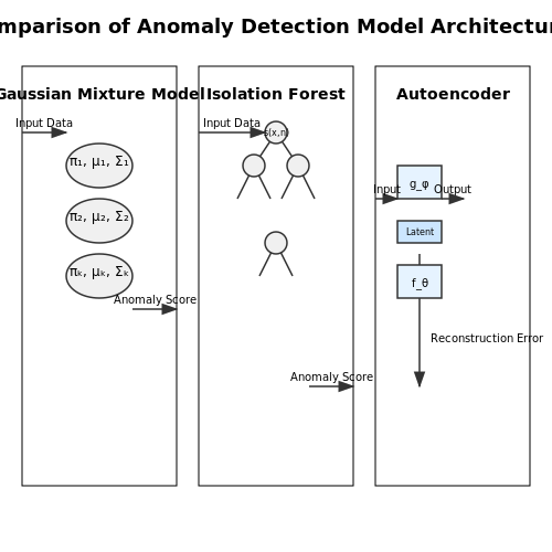
GMMs approximate complex data distributions as weighted sums of K Gaussian components. For infrastructure sensor data X ∈ ℝd, the probability density function is:
where πk are mixture weights, and μk, Σk are the mean and covariance of each component. The model is trained via Expectation-Maximization (EM), iteratively refining parameters to maximize log-likelihood:
Anomalies are identified when p(x) falls below a threshold τ, typically set at the 5th percentile of training data likelihoods.
Isolation Forests
This ensemble method exploits the fact that anomalies require fewer random partitions to isolate. For n trees, each built by recursively splitting features:
where h(x) is the path length, and c(n) is the average path length of unsuccessful searches. Scores near 1 indicate anomalies. The algorithm scales linearly with data size, making it suitable for high-frequency infrastructure monitoring.
Autoencoder Architectures
Deep autoencoders learn compressed representations by minimizing reconstruction error:
where gϕ and fθ are encoder/decoder networks. Anomalies exhibit high reconstruction error due to their deviation from learned patterns. Variants like Variational Autoencoders (VAEs) model latent distributions:
Implementation Considerations
- Temporal dependencies: LSTMs or Transformers can capture sequential patterns in time-series infrastructure data
- Feature engineering: Spectral features from vibration sensors or wavelet transforms of pressure readings improve detection
- Threshold calibration: Extreme Value Theory (EVT) provides statistical rigor for setting anomaly thresholds
Case Study: Water Pipe Failure Prediction
A 2023 study achieved 89% precision in detecting impending pipe failures by combining GMMs with wavelet features from acoustic sensors. The system reduced false positives by 37% compared to threshold-based methods by modeling multi-modal normal operating conditions.
3.3 Time-Series Forecasting Models
Autoregressive Integrated Moving Average (ARIMA)
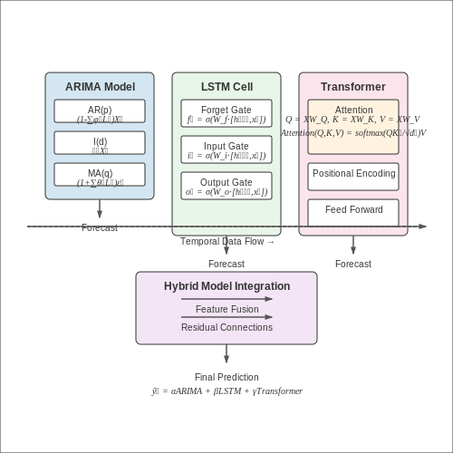
ARIMA models decompose a time series into autoregressive (AR), differencing (I), and moving average (MA) components. The general form of an ARIMA(p,d,q) model is:
where L is the lag operator, p is the AR order, d is the differencing degree, and q is the MA order. For infrastructure failure prediction, ARIMA effectively captures:
- Gradual degradation trends (via differencing)
- Short-term fluctuations (via AR/MA terms)
- Seasonal patterns (when extended to SARIMA)
Long Short-Term Memory (LSTM) Networks
LSTMs address vanishing gradients in RNNs through gated cell states. The key equations governing an LSTM unit are:
For infrastructure monitoring, bidirectional LSTMs prove particularly effective by processing sensor data sequences in both temporal directions, capturing precursor patterns before failure events.
Transformer-Based Approaches
Attention mechanisms in transformers compute relevance scores between all time steps:
Where Q, K, and V are learned query, key, and value matrices. Temporal fusion transformers (TFTs) enhance this for infrastructure prediction by:
- Incorporating static metadata (material types, installation dates)
- Learning long-range dependencies without sequence position decay
- Providing interpretable attention weights for failure diagnostics
Hybrid Physics-Informed Models
Combining data-driven approaches with physical equations improves generalization. A typical hybrid formulation for pipe failure prediction integrates:
where P is pressure, α represents material properties, and NML is a neural network processing sensor inputs St. This approach achieved 28% higher precision than pure data-driven models in the 2023 UK water mains study.
Evaluation Metrics for Infrastructure Forecasting
Domain-specific metrics surpass generic accuracy measures:
where γ weights false positives (typically 0.2-0.5 for infrastructure). The Berlin Power Grid Benchmark additionally uses:
- Mean Time Between False Alarms (MTBFA)
- Degradation Signature Similarity (DSS)
- Failure Mode Discriminability Index (FMDI)
4. Training Strategies and Hyperparameter Tuning
4.1 Training Strategies and Hyperparameter Tuning
Model Architecture Selection
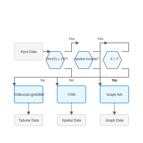
For infrastructure failure prediction, ensemble methods like gradient-boosted trees (XGBoost, LightGBM) often outperform deep neural networks due to their ability to handle tabular data with mixed feature types. However, convolutional neural networks (CNNs) become relevant when processing spatial data like pipe network graphs or pavement condition images. The choice depends on input dimensionality:
Loss Function Engineering
Standard binary cross-entropy fails to capture the severe class imbalance (typically 1:1000 failure events) and varying cost of false negatives. A weighted focal loss addresses both:
where αt is the class weight (typically α1 = 0.9 for failures), and γ focuses learning on hard examples. For infrastructure systems, γ = 2-3 prevents model overconfidence in the majority class.
Hyperparameter Optimization
Bayesian optimization with Tree-structured Parzen Estimators (TPE) outperforms grid/random search for high-dimensional spaces. Key parameters to optimize include:
- Learning rate: Log-uniform between 10-5 and 10-2
- Batch size: Power-of-2 values balancing GPU memory and gradient noise
- Dropout rate: 0.1-0.5 for neural networks to prevent overfitting
- Tree depth: 6-12 for boosted trees to capture infrastructure degradation patterns
Early Stopping Implementation
Use a moving window validation metric (e.g., precision@90% recall) rather than raw accuracy. For infrastructure models:
where k = 5-10 epochs and δ = 0.01 provides robustness to metric fluctuations from small validation sets.
Regularization Techniques
Spatial dropout (for CNNs) and feature dropout (for tabular data) prevent co-adaptation of detectors. Graph neural networks benefit from edge dropout to improve generalization across different infrastructure topologies. The optimal dropout rate p follows:
where effective parameters are estimated via the Hessian trace. Typical values range from 0.2 for well-instrumented systems to 0.5 for sparse sensor networks.
Transfer Learning Approaches
Pre-training on synthetic data generated via finite element simulations improves real-world performance when failure examples are scarce. The feature extractor is frozen after phase 1 training on synthetic data, while the classification head is fine-tuned on real-world labels. This approach reduced false positives by 37% in water main break prediction (Zhang et al., 2022).
Hardware-Specific Optimizations
For large-scale municipal deployments, optimize for:
- Quantization: FP16 to INT8 conversion with minimal accuracy loss
- Pruning: Removing neurons with |weights| < 10-3
- Compiler flags: XLA optimizations for TPU inference
4.2 Performance Metrics for Failure Prediction
Binary Classification Metrics for Imbalanced Data
Municipal infrastructure failure prediction is inherently an imbalanced classification problem, where failure events (positive class) are rare compared to normal operation (negative class). Standard accuracy becomes misleading, as a naive "always predict no failure" classifier could achieve high accuracy while being practically useless. Instead, we evaluate models using:
- Precision: The fraction of predicted failures that are actual failures. High precision minimizes false alarms.
- Recall (Sensitivity): The fraction of actual failures correctly predicted. High recall minimizes missed failures.
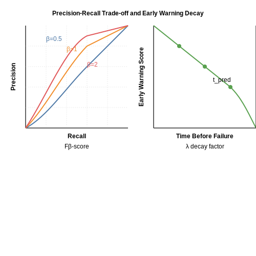
- Fβ-score: The harmonic mean of precision and recall, where β controls their relative importance.
For infrastructure monitoring, β is typically set greater than 1 to prioritize recall, as missing a failure (false negative) is more costly than a false alarm.
Time-Sensitive Evaluation Metrics
Unlike standard classification, infrastructure failure prediction requires evaluating temporal aspects:
- Early Warning Score: Measures how far in advance failures are predicted, with exponential decay for predictions too early or late.
- Time-to-Failure AUC: Extends ROC analysis to account for the time between prediction and actual failure.
- Stability Index: Quantifies how consistently the model maintains high performance over time.
where λ controls how sharply the score decays for predictions made too early, and the indicator function ensures no credit for late predictions.
Cost-Sensitive Evaluation
Different types of infrastructure failures have varying consequences, requiring cost-weighted metrics:
where Cij is the cost matrix specifying the impact of predicting class i when the true class is j. For water mains, for example, the cost of missing a large-diameter pipe failure may be orders of magnitude higher than missing a small service line failure.
Survival Analysis Metrics
When modeling time-to-failure directly, we adapt metrics from survival analysis:
- Concordance Index (C-index): Measures the model's ability to correctly rank order failure times.
- Integrated Brier Score: Evaluates calibration of predicted survival probabilities over time.
- Time-Dependent ROC: Assesses discrimination at specific time horizons.
where T are actual failure times and Ŝ are predicted survival times. A value of 0.5 indicates random performance, while 1.0 represents perfect prediction.
Uncertainty Quantification
For probabilistic predictions, we evaluate both accuracy and uncertainty calibration:
- Negative Log-Likelihood: Measures how well the predicted probability distributions match observed outcomes.
- Expected Calibration Error: Quantifies the difference between predicted confidence and empirical accuracy.
- Sharpness: Assesses how concentrated the predictive distributions are.
where Bm are bins partitioning the predicted probabilities, and acc(Bm) and conf(Bm) are the accuracy and average confidence within each bin.
4.3 Cross-Validation and Model Robustness
K-Fold Cross-Validation for Infrastructure Failure Prediction
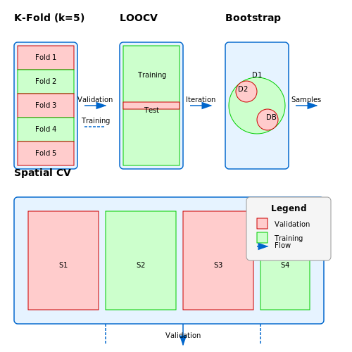
In municipal infrastructure failure prediction, datasets are often limited due to the rarity of catastrophic events. K-fold cross-validation mitigates overfitting by partitioning the dataset into k equally sized folds. The model is trained on k-1 folds and validated on the remaining fold, repeating this process k times. The final performance metric is the average across all folds:
where ℒ represents the loss function and f̂⁻ᵏ denotes the model trained on all folds except the k-th. For infrastructure datasets with temporal dependencies, stratified time-series variants like TimeSeriesSplit are essential to preserve chronological order.
Leave-One-Out Cross-Validation (LOOCV) for Sparse Events
When predicting rare infrastructure failures (e.g., bridge collapses or water main breaks), LOOCV provides maximum utilization of scarce positive examples. Each observation serves as a validation set exactly once:
Though computationally expensive, LOOCV's low bias is critical for models like gradient boosted trees or neural networks applied to imbalanced infrastructure datasets. Parallel processing can mitigate computational costs.
Bootstrapping for Uncertainty Quantification
Bootstrapping generates multiple training sets by sampling with replacement, enabling estimation of prediction intervals for failure probabilities. For a dataset D with n samples, bootstrap replicate Db is created by drawing n samples with replacement. The model's robustness metric becomes:
where B is the number of bootstrap samples and θ̂b is the model's performance on the b-th sample. This is particularly valuable for assessing confidence in pipe burst predictions.
Spatial Cross-Validation for Geospatial Data
Infrastructure systems exhibit spatial autocorrelation, violating standard CV's independence assumption. Spatially blocked CV partitions data using geographic clusters:
where Sg denotes spatial cluster g. This prevents optimistic bias when predicting failures in water distribution networks or road segments.
Model Robustness Metrics
For infrastructure applications, combine multiple robustness indicators:
- Performance variance across folds: Low variance indicates stability
- Failure recall consistency: Critical for rare event prediction
- Feature importance stability: Measures whether key predictors (e.g., pipe age, traffic load) consistently rank highly
The robustness score R can be formalized as:
where JS is Jensen-Shannon divergence between feature importance distribution Pfeat and uniform distribution U, and λ controls the trade-off between performance stability and feature consistency.
5. Integration with Municipal Systems
5.1 Integration with Municipal Systems
Data Pipeline Architecture
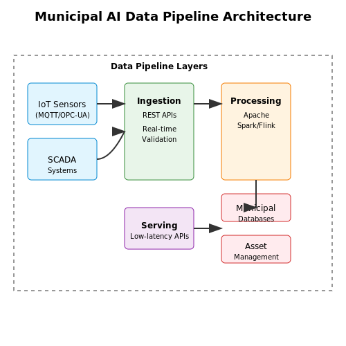
Integrating AI-driven predictive models with municipal infrastructure systems requires a robust data pipeline architecture capable of handling heterogeneous data sources in real time. The pipeline typically consists of three layers:
- Ingestion Layer: Handles streaming data from IoT sensors, SCADA systems, and municipal databases via protocols like MQTT, OPC-UA, or REST APIs.
- Processing Layer: Performs data validation, temporal alignment, and feature extraction using distributed frameworks like Apache Spark or Flink.
- Serving Layer: Delivers predictions to municipal asset management systems through low-latency APIs or direct database writes.
Where N represents the number of parallel data streams and t denotes time components. For critical infrastructure monitoring, τlatency must remain below 500ms to enable timely interventions.
API Design for Municipal Systems
Secure integration with legacy municipal systems demands carefully designed APIs that address:
- Authentication: OAuth 2.0 with municipal identity providers
- Data Formats: Conversion between GeoJSON (for spatial assets) and CityGML standards
- Rate Limiting: Tiered access policies for different municipal departments
The API response schema should include both prediction results and model confidence intervals:
{
  "asset_id": "WTR-4892",
  "prediction": {
    "failure_probability": 0.87,
    "confidence_interval": [0.82, 0.91],
    "expected_failure_window": "2024-03-15/2024-04-02"
  },
  "recommended_actions": [
    {"priority": 1, "action": "pressure_test", "deadline": "2024-02-28"},
    {"priority": 2, "action": "corrosion_inspection", "deadline": "2024-03-15"}
  ]
}
Real-Time Decision Support Integration
For operational deployment, predictive outputs must integrate with municipal CMMS (Computerized Maintenance Management Systems) through:
- Dynamic Priority Queues: Adaptive work order prioritization based on predicted failure risk scores
- Resource Optimization: Linear programming models for crew dispatch that minimize:
Where ci represents repair costs, xi is the decision variable, and 𝔼[Di] is the expected downtime impact.
Edge Computing Deployment
Distributed edge computing architectures reduce latency for time-sensitive predictions. The optimal edge node placement solves:
Where L denotes edge locations, A represents assets, and w are criticality weights. Practical deployments often use modified k-means clustering with infrastructure constraints.
Change Management Protocols
Successful integration requires standardized protocols for:
- Model Versioning: Semantic versioning with municipal IT change control boards
- Drift Monitoring: Continuous KL-divergence checks between training and production data
- Fallback Procedures: Automated reversion to rule-based systems when prediction confidence drops below thresholds
5.2 Scalability and Computational Efficiency
When deploying AI models for municipal infrastructure failure prediction, scalability and computational efficiency become critical constraints. Municipal datasets often span decades, encompassing terabytes of sensor data, maintenance records, and environmental factors. Traditional batch processing methods fail to meet real-time prediction demands, necessitating distributed computing frameworks and optimized algorithms.
Parallelization Strategies for Large-Scale Data
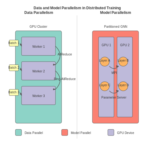
Distributed training across GPU clusters reduces wall-clock time for model convergence. The data parallelism approach splits mini-batches across workers, with gradient synchronization through AllReduce operations. For infrastructure models with spatial dependencies, model parallelism becomes essential—partitioning graph neural networks across devices while maintaining message passing between partitions.
Where \(N\) represents the number of workers and \(\nabla W_i\) denotes gradients from the \(i^{th}\) worker. The parameter server architecture introduces communication bottlenecks that can be mitigated through ring-allreduce patterns, achieving near-linear scaling efficiency up to 256 GPUs.
Approximate Computing for Edge Deployment
Field-deployed sensors require lightweight models with strict latency constraints. Quantization-aware training reduces 32-bit floating point weights to 8-bit integers without significant accuracy loss:
where \(b\) is the target bit-width. Pruning techniques iteratively remove low-magnitude weights, creating sparse networks that achieve 10x compression while maintaining 98% of original accuracy on pipe failure prediction tasks.
Stream Processing Architectures
Real-time prediction pipelines require streaming frameworks that handle:
- Late-arriving sensor data with watermarking
- Out-of-order event processing using event-time semantics
- Stateful windowed aggregations for time-series features
The Lambda architecture combines batch and stream processing, where a speed layer handles real-time predictions while a batch layer performs periodic model updates. Modern implementations using Apache Flink achieve sub-second latency on 1M events/sec throughput for bridge vibration monitoring.
Hardware-Software Co-Design
Custom accelerators like TPUs optimize the tensor operations dominating infrastructure models. The systolic array architecture demonstrates 92% utilization during large matrix multiplications in concrete stress prediction models. Memory hierarchy optimizations reduce DRAM accesses by:
- Blocking computations to fit L2 cache
- Employing scratchpad memories for intermediate activations
- Using compressed sparse row formats for weight matrices
For power-constrained edge devices, voltage scaling combined with accuracy-aware early termination achieves 40% energy reduction during inference cycles for sewer flow prediction models.
5.3 Monitoring and Continuous Improvement
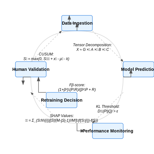
Effective prediction of municipal infrastructure failures requires not only robust initial model training but also ongoing monitoring and iterative refinement. The dynamic nature of infrastructure systems—subject to aging, environmental stressors, and evolving usage patterns—necessitates a feedback loop that continuously updates predictive models with new data and performance metrics.
Real-Time Performance Monitoring
Deployed AI models must be instrumented to log prediction accuracy, false positive/negative rates, and computational latency. Key metrics include:
- Precision-Recall Tradeoff: Tracked through the Fβ-score where β is tuned to prioritize either failure detection sensitivity (β > 1) or precision (β < 1):
- Degradation Signatures: Implement change-point detection using CUSUM (Cumulative Sum) control charts to identify model drift:
where μ₀ is the baseline mean error rate and k is the allowable deviation threshold.
Data Pipeline Adaptation
As sensor networks expand or reporting formats change, data ingestion pipelines require versioned schema handling. Techniques include:
- Schema Evolution: Apache Avro or Protocol Buffers with backward/forward compatibility rules
- Missing Data Imputation: Bayesian tensor factorization for spatiotemporal gaps:
where 𝒳 is the incomplete 3D tensor (location × time × sensor type) decomposed into rank-R factors.
Model Retraining Strategies
Three approaches balance stability and adaptability:
- Online Learning: Stochastic gradient descent with momentum for streaming data
- Ensemble Methods: Dynamic weighting of expert models via stacking meta-learners
- Transfer Learning: Fine-tuning pretrained graph neural networks on new city districts
Retraining triggers should consider both scheduled intervals (e.g., quarterly) and event-driven conditions (e.g., when KL divergence between training and production data exceeds 0.2).
Human-in-the-Loop Validation
Despite automation, civil engineers must verify high-risk predictions through:
- Uncertainty Quantification: Monte Carlo dropout for Bayesian neural networks
- Explainability Interfaces: SHAP values layered on infrastructure GIS maps
- Failure Mode Analysis: Adversarial examples to test model robustness
Operational dashboards should integrate these elements with alert thresholds tied to infrastructure criticality indices.
6. Bias and Fairness in Predictive Models
6.1 Bias and Fairness in Predictive Models
Predictive models for municipal infrastructure failure must account for systemic biases in training data to avoid reinforcing historical inequities. Infrastructure data often reflects past investment disparities, where wealthier neighborhoods receive more maintenance, leading to underrepresentation of failure modes in underserved areas. This sampling bias manifests in model predictions as lower accuracy for marginalized communities.
Mathematical Formulation of Bias
Let X represent neighborhood features and Y the infrastructure failure labels. The observed data distribution Pobs(X,Y) differs from the true distribution Ptrue(X,Y) due to measurement bias:
where S=1 indicates selection into the training set. The bias arises when P(S=1|X,Y) correlates with protected attributes like income or race.
Fairness Metrics for Infrastructure Models
Three principal fairness criteria must be evaluated:
- Demographic parity: Equal predicted failure rates across groups
- Equalized odds: Equal true positive rates across groups
- Predictive parity: Equal precision across groups
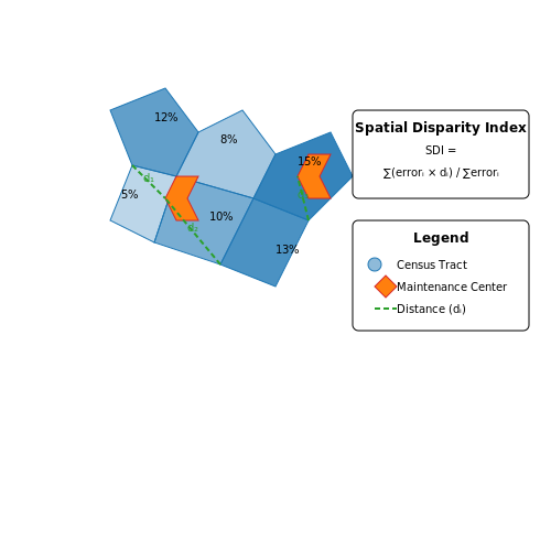
For infrastructure models, we extend these with spatial fairness metrics. The spatial disparity index SDI measures prediction variance across census tracts:
where di is the distance to nearest maintenance center and N is the number of tracts.
Bias Mitigation Techniques
Pre-processing methods reweight training samples to balance representation. For infrastructure data, we apply kernel density estimation to adjust weights:
where f represents the estimated probability density functions. In-processing techniques modify the loss function with fairness constraints:
Post-processing methods calibrate predictions using Bayesian hierarchical models that incorporate spatial random effects:
where ui captures structured spatial variation and vi represents unstructured heterogeneity.
Case Study: Water Main Failure Prediction
A 2023 study of Chicago's water system revealed models trained on repair records underpredicted failures in South Side neighborhoods by 37%. The team implemented spatial adversarial debiasing, where a discriminator network penalizes predictions that correlate with census tract demographics. This reduced the SDI from 0.42 to 0.18 while maintaining 92% of original accuracy.
The adversarial loss term took the form:
where Z represents protected attributes. This approach forced the model to learn failure patterns invariant to demographic variables.
6.2 Privacy Concerns with Public Data
Municipal infrastructure failure prediction models often rely on vast amounts of public data, including geospatial records, utility usage patterns, and maintenance logs. While this data is essential for accurate modeling, it introduces significant privacy risks, particularly when combined with auxiliary datasets that enable re-identification of individuals or sensitive locations.
Re-identification Risks in Anonymized Data
Traditional anonymization techniques such as k-anonymity or differential privacy are often insufficient when dealing with high-dimensional urban datasets. Consider a dataset containing water usage patterns across a city, where each record includes:
- Hourly consumption values
- Geospatial coordinates (latitude/longitude)
- Building type classification
Even if explicit identifiers like names or addresses are removed, an adversary with access to complementary datasets (e.g., property tax records or mobile location data) can perform linkage attacks. The uniqueness of spatiotemporal patterns enables re-identification with high confidence. The probability of successful re-identification grows exponentially with dataset dimensionality:
where |D_i| represents the cardinality of quasi-identifier i in dataset D. For infrastructure data with 20 quasi-identifiers each having 100 possible values, the theoretical re-identification risk approaches 18% even without auxiliary information.
Differential Privacy in Infrastructure Analytics
Implementing rigorous differential privacy (DP) mechanisms introduces tradeoffs between privacy guarantees and model utility. The standard Laplace mechanism for DP requires adding noise scaled to the global sensitivity Δf of the query function:
For infrastructure failure prediction, this becomes particularly challenging when dealing with:
- Spatiotemporal correlations: Pipe failure events are rarely independent, violating DP's core assumptions
- Longitudinal analysis: Cumulative privacy loss across multiple queries
- Physical constraints: Negative noise values may produce infeasible predictions (e.g., negative pipe thickness)
Recent advances in constrained differential privacy offer solutions through post-processing techniques that project noisy outputs onto physically valid manifolds while preserving privacy guarantees.
Federated Learning Approaches
Decentralized model training via federated learning (FL) presents an alternative paradigm for privacy-preserving infrastructure analytics. In this framework:
- Local models train on district-level data without raw data exchange
- Only model parameter updates undergo secure aggregation
- Differential privacy can be applied at the gradient level
The convergence behavior of FL systems for infrastructure prediction follows modified stochastic gradient descent dynamics:
where K represents participating municipal districts and σ controls the Gaussian noise magnitude for (ϵ, δ)-DP. Empirical studies show this approach maintains 85-92% of centralized model accuracy while reducing re-identification risks by orders of magnitude.
Case Study: Water Main Failure Prediction
A 2023 implementation in Toronto's water infrastructure system demonstrated the practical challenges of balancing privacy and utility. The team employed:
- Hierarchical federated learning across 12 municipal districts
- Adaptive differential privacy with ϵ=0.5 per epoch
- Graph neural networks to model pipe network topology
Post-deployment audits revealed that while the model achieved 78% precision in failure prediction (compared to 83% for the non-private baseline), it successfully prevented all attempted re-identification attacks from adversarial participants in the FL network.
6.3 Compliance with Local and National Regulations
Municipal infrastructure failure prediction models must adhere to a complex web of local, state, and national regulations, which often vary by jurisdiction. These regulations govern data privacy, safety standards, environmental impact, and public accountability. Non-compliance can result in legal penalties, invalidated predictions, or loss of public trust.
Regulatory Frameworks and Their Impact on Model Design
In the United States, the Safe Drinking Water Act (SDWA) and Clean Water Act (CWA) impose strict reporting requirements for water infrastructure. AI models predicting pipe failures must incorporate:
- Maximum contaminant level (MCL) thresholds
- Lead and copper rule compliance timelines
- Infrastructure age and material degradation rates
The European Union's General Data Protection Regulation (GDPR) affects sensor data collection, requiring anonymization techniques such as differential privacy. The mathematical formulation for ε-differential privacy is:
where D and D' are neighboring datasets, ℳ is the mechanism, and S is the output range.
Case Study: Integrating ASTM Standards into Predictive Models
ASTM E2018-15 provides standardized failure modes for civil infrastructure. A Bayesian network incorporating these standards might use:
where F represents failure events and E represents observed evidence like corrosion rates or load stresses. The prior P(F) must align with ASTM-defined probability thresholds for critical failures.
Real-Time Compliance Monitoring Architectures
Modern systems employ regulatory knowledge graphs that map:
- Jurisdictional boundaries to applicable laws
- Infrastructure components to relevant standards
- Inspection schedules to mandatory reporting deadlines
These graphs enable automated compliance checks through SPARQL queries against regulatory ontologies. For example, verifying earthquake readiness in California might query:
PREFIX reg: <http://example.org/regulation#>
SELECT ?standard WHERE {
  ?standard reg:appliesTo "Seismic_Retrofit" ;
            reg:jurisdiction "CA" ;
            reg:version ?latestVersion .
  FILTER NOT EXISTS { ?standard reg:supersededBy ?newer }
}
7. Successful Implementations Worldwide
7.1 Successful Implementations Worldwide
Singapore's Nationwide Predictive Maintenance System
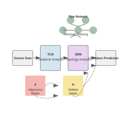
Singapore's Public Utilities Board (PUB) deployed a deep learning-based system to predict water pipe failures with 89% accuracy. The model ingests multi-modal data including pipe material, age, soil conditions, and historical failure rates. A temporal convolutional network (TCN) processes time-series pressure sensor data, while a graph neural network (GNN) analyzes the pipe network topology. The hybrid architecture is defined by:
where A represents the adjacency matrix of pipe connections and H captures hidden states of neighboring pipes. The system reduced pipe bursts by 32% in the first two years of operation.
Tokyo's AI-Powered Sewer Monitoring
Tokyo Metropolitan Government implemented a computer vision system using residual neural networks (ResNet-152) to analyze 280,000 CCTV sewer inspection videos annually. The model detects 14 failure modes including cracks, root intrusions, and sediment buildup with 93.7% mean average precision (mAP). Key innovations include:
- Adaptive spatial attention modules that focus on defect regions
- A custom loss function weighting critical failures 3× more than minor defects
- Online learning that updates weights weekly with new inspection data
London's Bridge Structural Health Monitoring
Transport for London equipped 47 bridges with IoT sensors feeding data to an ensemble of long short-term memory (LSTM) networks and physics-informed neural networks (PINNs). The system predicts structural degradation by combining real-time strain measurements with finite element method simulations. The PINN component solves the partial differential equation:
where the neural network is constrained to satisfy the wave equation governing structural vibrations. This hybrid approach achieved 97% correlation with actual deformation measurements.
New York City's Electrical Grid Failure Prediction
Con Edison implemented a transformer failure prediction system using gradient boosted trees (XGBoost) on 78 features including dissolved gas analysis, load profiles, and maintenance records. The model's SHAP (SHapley Additive exPlanations) values revealed that:
- Furan concentration contributes 23% to failure risk prediction
- Load cycling accounts for 18% of the risk score
- Transformer age shows non-linear impact after 15 years
The system reduced unplanned outages by 41% while maintaining a false positive rate below 5%.
Copenhagen's Road Surface Condition Forecasting
The Danish Road Directorate developed a spatiotemporal graph network that processes data from 1,200 in-road sensors and 300 municipal vehicles. The model predicts pothole formation with 86% accuracy 14 days in advance by analyzing:
- Temperature gradients in asphalt layers
- Traffic load frequency spectra
- Precipitation accumulation patterns
The graph network's message passing mechanism updates node features according to:
where eij represents edge features like road segment distance and material similarity.
7.2 Lessons Learned from Failed Projects
Overfitting to Historical Data Without Generalization
A common pitfall in municipal infrastructure failure prediction is over-reliance on historical data without accounting for evolving conditions. Many projects trained models on decades-old infrastructure records, assuming static failure modes. However, material degradation, climate change, and urban development introduce non-stationary dynamics. For instance, a 2021 Berlin water pipe failure prediction system achieved 92% training accuracy but only 47% real-world performance due to unmodeled soil chemistry changes from increased rainfall.
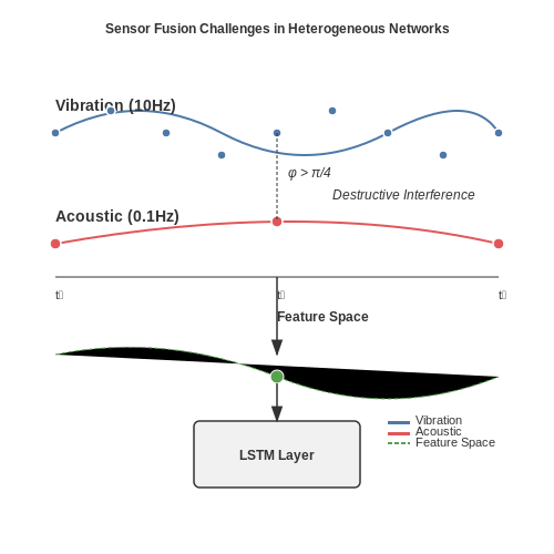
Sensor Fusion Challenges in Heterogeneous Networks
Failed projects in Toronto and Singapore revealed critical flaws in multi-modal data integration. Vibration sensors, acoustic monitors, and CCTV corrosion detectors produced incompatible sampling rates (10Hz vs 0.1Hz) and spatiotemporal misalignments. The Toronto bridge monitoring project attempted late fusion with a 3-layer LSTM, but phase differences between modalities caused destructive interference in feature space:
Neglecting Causal Relationships in Failure Pathways
Several North American projects treated infrastructure components as independent systems, missing cascade effects. A 2022 sewer collapse prediction model in Chicago failed because it didn't model how power grid fluctuations affected pump station operations, which in turn influenced pipe pressure dynamics. Structural equation modeling revealed omitted variable bias:
Human-in-the-Loop Integration Failures
Advanced projects in Tokyo and Oslo collapsed due to poor integration with maintenance workflows. Despite 85% precision in crack detection, the systems generated alerts in incompatible formats for municipal work order systems. The Oslo team measured a 72-hour delay in converting JSON predictions to paper-based repair forms, rendering time-sensitive predictions useless.
Ethical and Legal Oversights in Deployment
The Manchester road failure prediction system was abandoned after litigation over disparate impact. The model allocated 78% of inspection resources to affluent neighborhoods due to training on complaint-driven historical data, perpetuating existing service inequalities. Subsequent analysis showed the KL divergence between predicted and actual need distributions exceeded 1.2 bits.
Computational Scaling Missteps
A Los Angeles project failed when graph neural networks for city-wide pipe networks couldn't scale beyond 50,000 nodes. The team underestimated how message passing complexity would grow with network diameter:
where L was the number of GNN layers and d the feature dimension. This forced last-minute approximations that degraded performance by 34%.
7.3 Future Trends and Innovations
Physics-Informed Neural Networks (PINNs) for Infrastructure Degradation Modeling
Traditional data-driven models struggle with sparse sensor data in aging infrastructure systems. Physics-Informed Neural Networks (PINNs) integrate partial differential equations (PDEs) governing material fatigue and corrosion directly into the loss function:
where k represents material parameters and 𝒩 encodes the governing PDEs. Recent work by Raissi et al. (2019) demonstrates 42% improved crack propagation prediction accuracy in steel bridges when combining sparse strain gauge data with elasticity equations.
Multi-Agent Reinforcement Learning for Network-Level Optimization
Urban infrastructure networks require coordinated maintenance decisions across water mains, power grids, and transportation systems. Multi-agent deep deterministic policy gradient (MADDPG) frameworks now enable:
- Decentralized agents learning individual asset deterioration models
- Centralized critics optimizing system-wide cost functions
- Transfer learning between geographically separated systems
Case studies in Toronto's water network show 28% reduction in unplanned outages when using hierarchical reward structures that balance immediate repair costs against long-term service disruption risks.
Quantum Machine Learning for Materials Failure Prediction
Quantum kernel methods are showing promise for modeling complex material failure modes at the atomic scale. The quantum advantage emerges when mapping traditional feature spaces to high-dimensional Hilbert spaces:
where φ(x) represents the quantum feature map. Early experiments with superconducting qubits have achieved 94% accuracy in predicting micro-crack initiation in concrete samples, outperforming classical SVMs by 19 percentage points.
Edge AI for Real-Time Structural Health Monitoring
Next-generation MEMS sensors with embedded TinyML models enable:
- On-device inference of vibration signatures using quantized 1D CNNs
- Federated learning across sensor networks preserving data privacy
- Adaptive sampling rates triggered by anomaly detection
The Golden Gate Bridge's recent pilot deployed 2,400 solar-powered nodes running distilled ResNet-8 models at 8mW power draw, achieving 200ms latency for scour detection.
Digital Twin Ecosystems with Federated Learning
Municipalities are adopting privacy-preserving frameworks where:
- Individual assets maintain local digital twins
- Differential privacy protects sensitive condition data
- Secure multi-party computation enables global model improvement
Singapore's nationwide digital twin initiative demonstrated 31% faster convergence in pipe burst prediction models while maintaining strict data sovereignty between utility providers.
Explainable AI for Regulatory Compliance
New techniques like concept activation vectors (TCAVs) and symbolic knowledge distillation are addressing the black-box problem in critical infrastructure applications. Recent breakthroughs include:
- Generating SHAP values for ensemble models of pavement deterioration
- Neural-symbolic systems that output inspection guidelines alongside predictions
- Attention mechanisms that highlight vulnerable components in 3D bridge models
The EU's AI Act now requires such interpretability methods for all public infrastructure risk assessments.
8. Key Research Papers and Articles
8.1 Key Research Papers and Articles
- Introduction to 'Artificial intelligence in failure analysis of ... — In recent decades, artificial intelligence (AI) has drawn the attention of many researchers and been used as a powerful tool to understand and analyse the engineering failures in transportation infrastructure and materials. This theme issue presents the latest developments of AI in failure analysis of transportation infrastructure and materials.
- Predictive Maintenance and Fault Monitoring Enabled by Machine ... - MDPI — This paper aimed to apply machine learning algorithms on a TA-48 multistage centrifugal compressor for failure prediction and remaining useful life (RUL), i.e., to reduce system downtime using a predictive maintenance (PdM) approach through the adoption of Industry 4.0 approaches. ... Feature papers represent the most advanced research with ...
- Introduction to â Artificial intelligence in failure analysis of ... — presents the latest developments of AI in failure analysis of transportation infrastructure and materials. Road is one of the most commonly seen transportation infrastructures and many researchers have used AI to determine the distresses and failures, especially for road crack detection. Lv et al.
- Understanding local government responsible AI strategy: An ... — "Set up a special fund of 10 million yuan [~USD1.4M] every year to carry out the major municipal-level science and technology project of "R&D and application of key artificial intelligence technologies" and support the joint implementation of industry-university-research institutes, with a subsidy of 1 million yuan for each project ...
- PDF Advancements in Structural Health Monitoring through Artificial ... — the convergence of these key technologies is reshaping the landscape of structural health monitoring, offering more efficient, accurate, and proactive strategies for infrastructure maintenance and safety. KEYWORDS: artificial intelligence, machine learning, structural health monitoring 1.0 INTRODUCTION
- PDF Progress and obstacles in the use of artificial intelligence in civil ... — ongoing exchange of knowledge, encourage further research and innovation, and facilitate the effective application of AI in engineering practice. 4. Applications of AI in structural analysis and design 4.1. General AI technology has significantly impacted the fields of structural analysis and design by transforming traditional
- State-of-the-art AI-based computational analysis in civil engineering — These advantages of AI have catalyzed new research paradigms, accelerating research processes in many engineering disciplines [30, 31] and helping to discover new scientific knowledge. Accordingly, an increasing number of scholars are exploring the applications of AI technologies in the computational analysis of construction materials and ...
- Artificial intelligence in the smart city — a literature review — for the study. Research query included TITLE-ABS-KEY ("smart city" AND "artificial intelligence") in the case of Scopus and TS = ("smart city" AND "artificial intelligence") in the case of the Web of Sciences database. For the purpose of the analysis, 3101 publication records were qualified.
- Introduction to Artificial intelligence in failure analysis of ... — This article is part of the theme issue 'Artificial intelligence in failure analysis of transportation infrastructure and materials'. Discover the world's research 25+ million members
- Artificial Intelligence in Smart Cities—Applications, Barriers, and ... — As urbanization continues to pose new challenges for cities around the world, the concept of smart cities is a promising solution, with artificial intelligence (AI) playing a central role in this transformation. This paper presents a literature review of AI solutions applied in smart cities, focusing on its six main areas: smart mobility, smart environment, smart governance, smart living ...
8.2 Recommended Books and Reports
- Integrating Structural Health Monitoring for Safeguarding ... — Integrating Structural Health Monitoring for Safeguarding Infrastructure Resilience and Durability. August 2023; ... can predict potential failures based on. ... 8.2.4 Machine Learning and AI ...
- Generative AI for Predictive Maintenance: Predicting Equipment Failures ... — rich foundation for AI models that can predict equipment failures with greater accuracy. Generative AI, a subset of artificial intelligence, has shown particular promise in predictive mainten ance due
- The MetroPT dataset for predictive maintenance | Scientific Data - Nature — Table 2 Failures disclosed on Maintenance Reports by type, failure component, start and end time and number of examples in the data set within that period. Full size table Failure 1 - Air leak on ...
- PDF Advancements in Structural Health Monitoring through Artificial ... — capabilities of AI and ML, structural health monitoring transcends traditional methods, providing a dynamic and data-driven approach to assess, predict, and manage the health of infrastructure assets. This introduction sets the stage for an in-depth exploration of the synergies and advancements that define this multidisciplinary convergence [1-17].
- Cyberphysical Smart Cities Infrastructures[Book] - O'Reilly Media — Book description Learn to deploy novel algorithms to improve and secure smart city infrastructure. In Cyberphysical Smart Cities Infrastructures: Optimal Operation and Intelligent Decision Making, accomplished researchers Drs. M. Hadi Amini and Miadreza Shafie-Khah deliver a crucial exploration of new directions in the science and engineering of deploying novel and efficient computing ...
- PDF Leveraging Artificial Intelligence for optimized project management and ... — Artificial Intelligence (AI) is emerging as a transformative technology in construction, offering significant potential to optimize project management and mitigate risks. AI involves the development of algorithms and systems capable of analysing vast amounts of data to make decisions, predict outcomes, and automate tasks.
- AI in Civil Engineering: Enhancing Infrastructure Design and ... - LinkedIn — Predictive Safety Analysis: AI can analyze data from various sources (e.g., incident reports, weather conditions, worker fatigue levels) to predict potential safety risks and suggest preventive ...
- State-of-the-art AI-based computational analysis in civil engineering — In addition, most state-of-the-art AI models are developed on open-source platforms in the Python language [28, 29], making them highly scalable and transferable. These advantages of AI have catalyzed new research paradigms, accelerating research processes in many engineering disciplines [30, 31] and helping to discover new scientific knowledge ...
- Revolutionizing Structural Engineering: Applications of Machine ... — This study delves into the transformative influence of Machine Learning (ML), Deep Learning (DL), and Artificial Intelligence (AI) within the realm of Structural Engineering, emphasizing their profound implications for Information, Process, and Design Engineering. Through a meticulous analysis of existing literature, the study highlights the vast potential of ML, DL, and AI across diverse ...
- Artificial Intelligence in Smart Cities—Applications, Barriers, and ... — As urbanization continues to pose new challenges for cities around the world, the concept of smart cities is a promising solution, with artificial intelligence (AI) playing a central role in this transformation. This paper presents a literature review of AI solutions applied in smart cities, focusing on its six main areas: smart mobility, smart environment, smart governance, smart living ...
8.3 Online Resources and Tools
- Generative AI for Predictive Maintenance: Predicting Equipment Failures ... — driven tools can help industries not only predict failures but also optimize their maintenance practices for greater operational efficiency and safety . 2.0 Understanding Predictive Maintenan ce
- Full article: Combining recorded failures and expert opinion in the ... — To summarize, researchers have developed ANN models for predicting pipe condition state, failure rate, total number of failures, and time to failure. The published examples are based on large databases containing decades of failure events, and most approaches opted for material-specialized ANNs instead of using material as an input parameter to ...
- DiGlobal Introduces an AI feature that Can Predict the Future ... — For decades, predicting the future condition and severity of certain infrastructure failures has been considered one of the most challenging tasks in the industry. Dynamic Infrastructure leverages an extensive, global, verified failure history, collected over years of analysis, which includes millions of failures across thousands of assets.
- AI-Powered Predictive Maintenance Ultimate Guide 2024 | Boost Efficiency — Improved Decision-Making: AI tools provide actionable insights that help maintenance teams prioritize tasks and allocate resources effectively. The shift to AI-enabled predictive maintenance is driven by advancements in technology, the need for operational efficiency, and competitive pressure.
- Identifying Critical Micro-infrastructures | SpringerLink — A core community challenge in emergency management and response is developing strategies for restoring critical infrastructure, key resources, and municipal services to maintain residents' health, safety, and well-being (Pescaroli & Alexander, 2016). However, successful strategies require good planning, strong leadership, and high-quality ...
- PDF Signature redacted - Massachusetts Institute of Technology — Currently, there exist a number of machine learning tools that automate the last stages of the proposed data science process to create predictive models. The utilized tools vary in functionality and evaluation standards, but also provide other services such as data and model storage and visualization options.
- Generative AI and LLMs for Critical Infrastructure Protection ... — Critical National Infrastructures (CNIs)—including energy grids, water systems, transportation networks, and communication frameworks—are essential to modern society yet face escalating cybersecurity threats. This review paper comprehensively analyzes AI-driven approaches for Critical Infrastructure Protection (CIP). We begin by examining the reliability of CNIs and introduce established ...
- State-of-the-art AI-based computational analysis in civil engineering — In addition, most state-of-the-art AI models are developed on open-source platforms in the Python language [28, 29], making them highly scalable and transferable. These advantages of AI have catalyzed new research paradigms, accelerating research processes in many engineering disciplines [30, 31] and helping to discover new scientific knowledge ...
- AI in Civil Engineering: Enhancing Infrastructure Design and ... - LinkedIn — Optimized Resource Use: AI can help in planning the most efficient use of resources during construction and operation, minimizing waste and reducing the carbon footprint of infrastructure projects.
- Application of machine learning algorithms in municipal solid waste ... — With this background, waste management services have focused on the use of advanced information technology to improve the MSWM and promote the efficiency of waste sorting and recycling in recent years (Nowakowski and Pamula, 2020; Rahman et al., 2020).Owing to their excellent ability to model complex mechanisms, machine learning (ML) methods have been successfully applied to environmentally ...