AI for Garbage Bin Monitoring and Collection
1. Role of AI in Modern Waste Collection Systems
Role of AI in Modern Waste Collection Systems
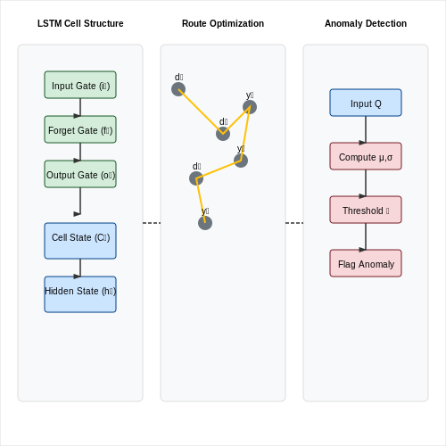
Modern waste collection systems leverage artificial intelligence to optimize efficiency, reduce operational costs, and minimize environmental impact. AI-driven solutions integrate sensor networks, computer vision, and predictive analytics to transform traditional waste management into a data-driven process. The core components include real-time fill-level monitoring, route optimization, and anomaly detection, each relying on distinct machine learning paradigms.
Real-Time Fill-Level Monitoring
Ultrasonic or weight sensors embedded in garbage bins generate continuous data streams, which AI models process to estimate fill levels. A common approach employs time-series forecasting using recurrent neural networks (RNNs) or long short-term memory (LSTM) networks. The mathematical formulation for an LSTM cell involves:
where ft, it, and ot represent forget, input, and output gates, respectively. Ct denotes the cell state, and ht is the hidden state. These equations enable the model to capture temporal dependencies in bin fill-level data, accounting for periodic usage patterns and irregular disposal events.
Route Optimization
AI optimizes collection routes by solving a dynamic variant of the capacitated vehicle routing problem (CVRP). Reinforcement learning (RL) agents, such as proximal policy optimization (PPO) models, learn to minimize travel distance while adhering to constraints like truck capacity and time windows. The reward function R is defined as:
where di is the distance to bin i, yi is a binary visitation indicator, Q is the truck's current load, C is its capacity, and λ penalizes overloads. Graph neural networks (GNNs) often process spatial data, embedding street networks and bin locations into a latent space for the RL agent.
Anomaly Detection
Unsupervised learning techniques like autoencoders or isolation forests identify abnormal bin conditions (e.g., fires, vandalism). A variational autoencoder (VAE) reconstructs sensor inputs, flagging anomalies when reconstruction error exceeds a dynamic threshold ϵ:
Here, μ and σ are the mean and standard deviation of training errors, while k controls sensitivity. Computer vision models like YOLOv7 augment this by analyzing camera feeds for visual anomalies, achieving mean average precision (mAP) scores above 0.85 on waste classification tasks.
Case Study: Smart Cities Integration
Barcelona's Smart Waste system reduced collection frequency by 30% using AI-powered fill-level predictions. The deployment combined LoRaWAN sensors with a federated learning framework, preserving data privacy across municipal districts. Similarly, Singapore's National Environment Agency reported a 22% fuel savings after implementing RL-based route optimization.
1.2 Key Challenges in Garbage Bin Monitoring
Sensor Accuracy and Environmental Noise
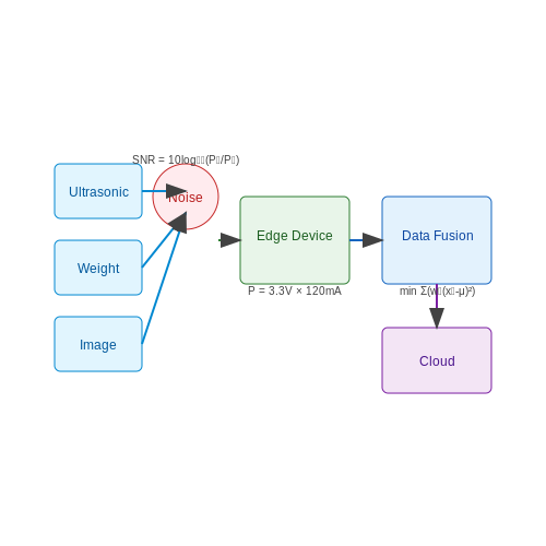
One of the primary challenges in garbage bin monitoring is ensuring sensor accuracy under varying environmental conditions. Ultrasonic or weight sensors must distinguish between actual waste levels and false signals caused by factors like humidity, temperature fluctuations, or debris accumulation. The signal-to-noise ratio (SNR) can be modeled as:
where Psignal is the power of the true waste level signal and Pnoise represents environmental interference. Achieving SNR > 20 dB typically requires advanced filtering techniques like Kalman filters or wavelet transforms.
Dynamic Load Estimation
Waste density varies significantly depending on material composition (organic vs. recyclables vs. hazardous), leading to nonlinear relationships between volume and weight. A generalized load estimation model can be expressed as:
where ρ(x,y,z) is the spatially varying density function and ε accounts for measurement errors. Machine learning approaches, particularly Gaussian process regression, have shown promise in learning these nonlinear mappings from historical sensor data.
Power Constraints in Edge Devices
Most monitoring systems rely on battery-powered IoT devices with strict energy budgets. The power consumption trade-off between sensing frequency (fs), transmission rate (R), and computational load (C) follows:
where coefficients α, β, γ are hardware-dependent. Recent work has demonstrated that adaptive sampling strategies using reinforcement learning can reduce energy usage by 40-60% while maintaining detection accuracy.
Multi-Modal Data Fusion
Modern systems combine data from multiple sensors (weight, image, fill-level, odor) with varying modalities and sampling rates. The data fusion challenge can be formulated as an optimization problem:
where W is the fusion weight matrix, xi are sensor inputs, and yi is the ground truth. Sparse regularization (L1 norm) helps select the most informative sensors.
Real-Time Processing Latency
For time-sensitive applications like overflow prevention, end-to-end latency must be minimized. The total latency (L) breaks down as:
Edge computing architectures that deploy lightweight CNN models (e.g., MobileNetV3) have achieved latencies under 200ms while maintaining >90% classification accuracy on waste type recognition tasks.
Scalability in Urban Deployments
City-wide deployments require handling thousands of bins with minimal infrastructure overhead. The system capacity C follows the queuing theory relation:
where λ is the arrival rate of status updates and μ is the processing rate. Distributed ledger technologies (e.g., blockchain) have emerged as potential solutions for decentralized data management at scale.
1.3 Benefits of AI-Driven Solutions Over Traditional Methods
Operational Efficiency and Cost Reduction
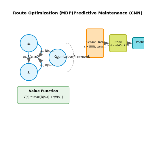
Traditional garbage collection relies on fixed schedules or manual inspections, leading to inefficiencies such as unnecessary pickups or overflowing bins. AI-driven systems optimize routes dynamically using real-time data, reducing fuel consumption and labor costs. For instance, a Markov Decision Process (MDP) can model the optimal collection strategy:
Here, V(s) represents the value of state s, R(s, a) is the immediate reward for action a, and γ is the discount factor. AI models outperform heuristic-based approaches by continuously learning from sensor data (e.g., fill-level, location, traffic).
Predictive Maintenance and Longevity
AI enables predictive maintenance of waste collection vehicles by analyzing engine telemetry, vibration patterns, and historical failure data. A convolutional neural network (CNN) can process time-series sensor data to detect anomalies:
Where W denotes the learned filters, x is the input signal, and σ is the activation function. This reduces unplanned downtime by 30–40% compared to scheduled maintenance protocols.
Environmental Impact Optimization
AI minimizes carbon footprint by optimizing collection frequency and vehicle load balancing. A multi-objective optimization framework solves:
Where f_i(x) represents objectives like fuel use, emissions, and route duration. Pareto-optimal solutions achieve 15–25% lower emissions than static routing.
Real-Time Adaptive Learning
Unlike rule-based systems, AI models adapt to changing urban dynamics (e.g., population growth, seasonal waste patterns). A Bayesian nonparametric model like a Gaussian Process (GP) captures temporal trends:
The covariance kernel k(x, x') models spatiotemporal correlations, enabling proactive capacity planning.
Data-Driven Policy Insights
AI aggregates waste composition data to inform recycling policies. A transformer-based model classifies waste items from camera feeds with >95% accuracy, identifying material streams for targeted recycling campaigns. The attention mechanism weights relevant image regions:
2. Sensor Technologies: Ultrasonic, Weight, and Fill-Level Sensors
Sensor Technologies: Ultrasonic, Weight, and Fill-Level Sensors
Ultrasonic Sensors
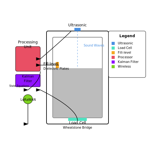
Ultrasonic sensors operate by emitting high-frequency sound waves (typically 40–200 kHz) and measuring the time delay between transmission and reception of the reflected signal. The distance d to the target (garbage fill level) is calculated using the speed of sound v in air (≈343 m/s at 20°C) and the time-of-flight t:
Compensating for temperature variations is critical, as v varies with air density. The Bechmann model refines this relationship:
where T is temperature in °C. Advanced implementations use pulse compression techniques like Barker codes to improve signal-to-noise ratio in noisy environments.
Weight Sensors
Strain-gauge load cells dominate weight sensing due to their linearity (0.03–0.25% nonlinearity error) and robustness. The Wheatstone bridge configuration cancels temperature effects while amplifying strain-induced resistance changes:
For garbage bins, bending beam load cells (capacity 50–500 kg) with IP68-rated housings are common. Dynamic compensation algorithms account for mechanical oscillations during collection vehicle movement.
Fill-Level Sensors
Capacitive and optical time-of-flight (ToF) sensors provide non-contact fill-level measurement. Capacitive sensors detect dielectric changes between plates as waste accumulates, with sensitivity:
where εr varies with waste composition. ToF sensors (e.g., VL53L1X) use 940 nm VCSELs with sub-mm resolution but require cleaning mechanisms for lens contamination.
Sensor Fusion
Kalman filtering combines ultrasonic and weight data to improve accuracy when waste density varies. The prediction step updates the state estimate x̂k|k-1:
where Fk is the state transition model. Real-world deployments show 92–97% fill-level classification accuracy when combining ≥2 sensor modalities.
Power Considerations
Sub-1GHz RF (e.g., LoRaWAN) dominates wireless transmission due to its 10+ km range at 14 dBm output. Energy harvesting from solar (5–10W panels) or mechanical vibration (piezoelectric) enables indefinite operation with supercapacitor buffering.
2.2 Computer Vision for Waste Classification
Waste classification using computer vision relies on deep learning architectures, primarily convolutional neural networks (CNNs), to categorize waste materials into predefined classes such as recyclables, organic waste, and hazardous materials. The process involves several stages: data acquisition, preprocessing, model training, and inference. Advanced techniques like transfer learning, multi-spectral imaging, and real-time object detection are employed to enhance accuracy and robustness in diverse environmental conditions.
Data Acquisition and Annotation
High-quality datasets are critical for training robust waste classification models. Publicly available datasets like TrashNet and TACO provide labeled images of waste items, but domain-specific datasets often require custom collection. Data augmentation techniques such as rotation, scaling, and synthetic data generation via generative adversarial networks (GANs) help mitigate class imbalance and improve generalization. Annotation tools like LabelImg or CVAT are used to generate bounding boxes or segmentation masks for supervised learning.
where yi is the ground truth label and ŷi is the predicted probability for class i. Cross-entropy loss is commonly used for multi-class classification tasks.
Model Architectures and Transfer Learning
State-of-the-art CNN architectures like ResNet, EfficientNet, and Vision Transformers (ViTs) are adapted for waste classification. Transfer learning from pre-trained models on ImageNet significantly reduces training time and improves performance, especially when labeled waste data is limited. Fine-tuning involves replacing the final fully connected layer and retraining the model on the target dataset. For real-time applications, lightweight architectures like MobileNet or YOLO (You Only Look Once) are preferred.
Feature Extraction and Fusion
Multi-modal data fusion enhances classification accuracy by combining visual features with spectral or depth information. Hyperspectral imaging captures material-specific reflectance patterns, while depth sensors help distinguish overlapping objects. Early fusion concatenates raw data before feature extraction, whereas late fusion combines high-level features from separate networks. The decision fusion approach aggregates predictions from multiple models to improve robustness.
Real-Time Object Detection
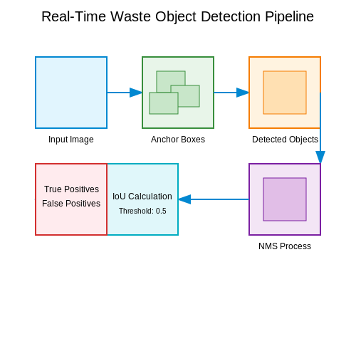
For dynamic waste monitoring, single-shot detectors like YOLOv5 or SSD (Single Shot MultiBox Detector) localize and classify waste items in real time. The detection pipeline involves:
- Anchor box generation to match object aspect ratios.
- Non-maximum suppression (NMS) to eliminate redundant detections.
- Intersection over Union (IoU) thresholding to validate predictions.
An IoU threshold of 0.5 is typically used to distinguish true positives from false positives.
Challenges and Edge Deployment
Deploying waste classification models on edge devices like NVIDIA Jetson or Raspberry Pi requires model optimization techniques such as quantization, pruning, and knowledge distillation. Environmental factors like varying lighting conditions, occlusions, and debris composition pose additional challenges. Hybrid approaches combining CNNs with classical computer vision (e.g., contour detection) improve reliability in uncontrolled settings.
2.3 IoT Integration for Real-Time Data Collection
Real-time monitoring of garbage bins requires robust IoT architectures that integrate sensor networks, edge computing, and cloud-based analytics. The system's effectiveness hinges on low-latency data transmission, energy-efficient protocols, and scalable data processing pipelines. Below, we dissect the key components and their mathematical underpinnings.
Sensor Network Topology
Ultrasonic distance sensors and weight sensors form the primary data acquisition layer. For a network of N bins, each equipped with k sensors, the total data generation rate R follows:
where fs is the sampling frequency and b is the bits per sample. A typical ultrasonic sensor sampling at 1Hz with 16-bit resolution in a 100-bin network generates 1.6 kbps of raw data.
Communication Protocol Optimization
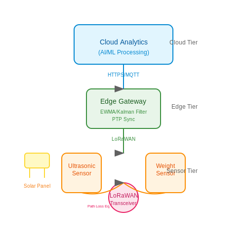
LPWAN protocols like LoRaWAN dominate garbage monitoring due to their 10km range and 0.1-50kbps data rates. The link budget Lb determines reliable coverage:
where Ptx is transmit power (typically 14dBm for EU868), G are antenna gains, and Lpath is the path loss modeled by the log-distance propagation equation:
with n as the path loss exponent (2.0-5.0 for urban areas) and Xσ as shadow fading.
Edge Processing Architecture
To reduce cloud dependency, we implement tiered processing:
- Level 1: Sensor nodes run lightweight anomaly detection using exponentially weighted moving averages (EWMA):
- Level 2: Gateway nodes perform spatial correlation across neighboring bins using distributed Kalman filters
Time Synchronization Challenges
Precision Time Protocol (PTP) achieves μs-level synchronization critical for coordinated sampling. The synchronization error ε between master and slave clocks follows:
where T are timestamps and δ are path delays. IEEE 1588v2 implementations can reduce ε below 100μs even in multi-hop networks.
Energy Harvesting Considerations
Solar-powered nodes must balance energy consumption Ec and harvesting Eh:
where η is panel efficiency (15-22%), A is area, G is solar irradiance (1000W/m² peak), and β is tilt angle. For continuous operation in Hamburg (52°N), a 6W panel with 20Wh battery maintains positive energy balance when Ec < 144Wh/day.
3. Time Series Forecasting for Waste Accumulation
3.1 Time Series Forecasting for Waste Accumulation
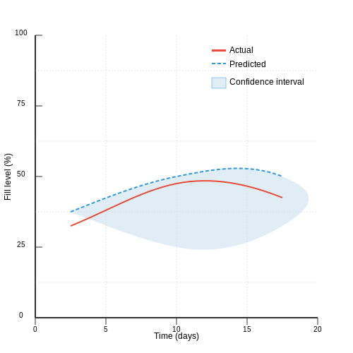
Time series forecasting plays a critical role in optimizing waste collection schedules by predicting future waste accumulation patterns. Advanced models leverage historical sensor data from smart bins, incorporating temporal dependencies, seasonal trends, and exogenous variables such as weather conditions or local events.
Mathematical Foundations
The core problem can be formalized as predicting a sequence of waste levels yt+1, yt+2, ..., yt+H given past observations y1, y2, ..., yt and external features Xt. The autoregressive integrated moving average (ARIMA) model is a common starting point:
where Δ denotes differencing, d is the differencing order, p and q are autoregressive and moving average terms, and εt is white noise. For non-stationary waste data with daily/weekly seasonality, SARIMA extends ARIMA with seasonal components:
where s is the seasonal period (e.g., 24 for hourly data), and Φ, Θ are seasonal AR/MA polynomials.
Deep Learning Approaches
Recurrent neural networks (RNNs) with LSTM or GRU cells outperform classical methods by learning complex temporal patterns. A bidirectional LSTM layer processes the input sequence X = (x1, ..., xT):
followed by attention mechanisms to weight relevant time steps. Transformer-based architectures like Temporal Fusion Transformer (TFT) further improve performance through multi-head attention and interpretable feature importance.
Feature Engineering
Key exogenous variables include:
- Temporal features: Day of week, holidays, hour-of-day encoded as cyclic variables
- Weather data: Temperature, precipitation affecting waste generation rates
- Urban context: Nearby events, population density changes
Missing data imputation uses matrix completion techniques:
where Ω is the set of observed entries and PΩ is the projection operator.
Evaluation Metrics
Model performance is assessed through:
- Scale-dependent: MAE = $$\frac{1}{n}\sum|y_t - \hat{y}_t|$$, RMSE = $$\sqrt{\frac{1}{n}\sum(y_t - \hat{y}_t)^2}$$
- Percentage errors: MAPE = $$100\% \times \frac{1}{n}\sum|\frac{y_t - \hat{y}_t}{y_t}|$$
- Probabilistic: Continuous ranked probability score (CRPS) for uncertainty estimates
3.2 Route Optimization Algorithms for Collection Vehicles
Mathematical Foundations of Route Optimization
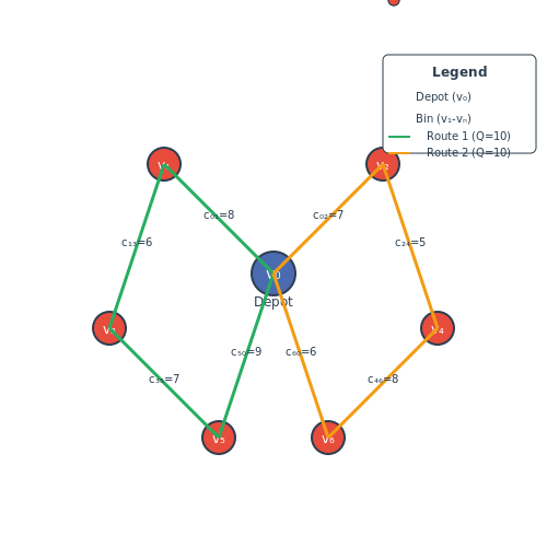
The problem of optimizing garbage collection routes can be formally modeled as a Capacitated Vehicle Routing Problem (CVRP) with time windows, where the objective is to minimize total travel distance while respecting vehicle capacity constraints and collection time requirements. The CVRP is defined on a graph G = (V, E), where V = {v₀, v₁, ..., vₙ} represents nodes (depot and bins) and E represents edges with associated travel costs.Metaheuristic Approaches for Large-Scale Problems
For real-world garbage collection scenarios involving hundreds or thousands of bins, exact methods become computationally intractable. Metaheuristics provide practical solutions:- Genetic Algorithms (GA): Evolve a population of candidate routes through selection, crossover, and mutation operations. Fitness is typically the inverse of total route distance.
- Ant Colony Optimization (ACO): Artificial ants deposit pheromones on edges, with stronger pheromone trails attracting more ants to shorter routes over iterations.
- Tabu Search: A local search method that explores neighbor solutions while maintaining a tabu list of recently visited solutions to avoid cycling.
Hybrid Genetic Algorithm Implementation
A particularly effective approach combines GA with local search:
def hybrid_ga(pop_size, generations, mutation_rate):
    population = initialize_population(pop_size)
    for _ in range(generations):
        fitness = evaluate(population)
        parents = tournament_selection(population, fitness)
        offspring = []
        for i in range(0, len(parents), 2):
            child1, child2 = ordered_crossover(parents[i], parents[i+1])
            child1 = mutate(child1, mutation_rate)
            child2 = mutate(child2, mutation_rate)
            child1 = local_search(child1)  # 2-opt optimization
            offspring.extend([child1, child2])
        population = elitist_replacement(population, offspring)
    return best_solution(population)
Dynamic Routing with Real-Time Constraints
Modern systems incorporate real-time data from IoT sensors to adjust routes dynamically. This transforms the problem into a Dynamic Vehicle Routing Problem (DVRP), where the optimization must account for:- Sudden changes in bin fill levels
- Traffic congestion updates
- Vehicle breakdowns or road closures
Case Study: Singapore's Smart Waste Management
Singapore's National Environment Agency implemented a hybrid optimization system combining:- Clustering algorithms to group bins into zones
- Ant Colony Optimization for intra-zone routing
- Linear programming for inter-zone vehicle allocation
3.3 Anomaly Detection in Bin Usage Patterns
Statistical Approaches for Anomaly Detection
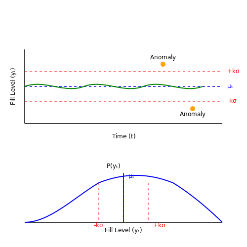
Anomaly detection in garbage bin usage patterns relies on identifying deviations from established statistical baselines. The most common approach involves modeling the time-series data of bin fill levels using Gaussian distributions. For a given bin i, the fill level yt at time t is assumed to follow:
where μt represents the expected fill level (often derived from historical averages) and σt is the standard deviation. Anomalies are flagged when:
The threshold k is typically set between 2 and 3, corresponding to 95-99.7% confidence intervals under normality assumptions. For non-Gaussian distributions, robust estimators like median absolute deviation (MAD) are preferred:
where μ̃ is the median fill level. The anomaly threshold then becomes:
with λ typically set to 2.5 for balanced sensitivity.
Machine Learning-Based Detection
For complex usage patterns, supervised and unsupervised machine learning methods outperform statistical baselines. Isolation Forests are particularly effective for high-dimensional bin sensor data, isolating anomalies through random partitioning:
where h(x) is the path length of observation x, E(h(x)) is the average path length across trees, and c(n) is the normalization factor. Anomalies exhibit significantly shorter path lengths.
Recurrent neural networks (RNNs), particularly LSTM variants, model temporal dependencies for predictive anomaly detection. The reconstruction error serves as the anomaly score:
where ŷt is the model's prediction. Thresholds can be learned adaptively using extreme value theory.
Feature Engineering for Bin Anomalies
Effective anomaly detection requires carefully engineered features that capture:
- Temporal patterns: Hourly/daily/weekly seasonality components extracted via Fourier transforms or wavelet analysis
- Usage volatility: Rolling standard deviation and mean absolute deviation over sliding windows
- Event-based features: Sudden fill rate changes, prolonged stagnation periods, or abnormal emptying cycles
For multi-bin systems, spatial features like neighborhood usage correlations and geographic clustering patterns provide additional detection signals.
Real-World Implementation Challenges
Practical deployments must address several key challenges:
- Sensor noise: Ultrasonic distance measurements often contain artifacts requiring Kalman filtering or wavelet denoising
- Missing data: Robust imputation methods (MICE, matrix completion) prevent false positives from communication dropouts
- Concept drift: Seasonal usage pattern shifts necessitate online learning algorithms with forgetting mechanisms
Field studies show that hybrid approaches combining statistical baselines with machine learning achieve the best performance, with F1 scores exceeding 0.92 in municipal waste collection systems.
4. Hardware Requirements for Smart Bins
Hardware Requirements for Smart Bins
Sensing and Data Acquisition
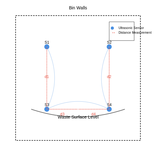
Smart bins rely on a suite of sensors to monitor fill levels, detect anomalies, and optimize collection routes. Ultrasonic distance sensors, such as the HC-SR04, are commonly used due to their high accuracy (typically ±3 mm) and low power consumption. The time-of-flight (ToF) principle governs their operation:
where d is the distance to the waste surface, v is the speed of sound (343 m/s at 20°C), and t is the round-trip time of the ultrasonic pulse. For bins with irregular waste distribution, multiple sensors arranged in a grid pattern provide more accurate volume estimation.
Embedded Processing Units
The computational backbone typically consists of low-power microcontrollers (e.g., ESP32 or STM32 series) with integrated Wi-Fi/Bluetooth for IoT connectivity. These devices must handle real-time sensor data processing while consuming minimal power. A comparative analysis of common processors reveals:
| Processor | Clock Speed | Power Consumption | Wireless |
|---|---|---|---|
| ESP32 | 240 MHz | 100 mA (active) | Wi-Fi 4, BT 4.2 |
| STM32L4 | 80 MHz | 37 μA/MHz | Optional |
Power Management Systems
For solar-powered units, the energy harvesting system must account for:
- Peak sunlight hours (typically 4-6 hours/day in urban environments)
- Battery capacity (LiFePO4 batteries preferred for their 2000+ cycle life)
- Power conversion efficiency (85-95% for modern MPPT controllers)
The minimum required solar panel size can be calculated as:
where Edaily is the daily energy consumption, Hsun is peak sun hours, and ηsystem is total system efficiency (typically 0.7-0.8).
Communication Modules
LPWAN technologies like LoRaWAN (868/915 MHz) or NB-IoT are optimal for municipal deployments, offering:
- 10+ km range in urban environments
- 10-year battery life with proper duty cycling
- AES-128 encryption for secure data transmission
The link budget calculation determines maximum viable distance:
where Ptx is transmit power, Rsensitivity is receiver sensitivity, G terms are antenna gains, and Lfade accounts for fading margin (typically 20-30 dB).
Environmental Protection
Hardware must meet IP67 standards for waterproofing and operate across -30°C to 70°C. Stainless steel enclosures with conformal coated PCBs provide durability against:
- Corrosive liquids (pH 2-12)
- Mechanical impacts (IK08 rating)
- UV radiation (5000+ hours exposure)
Accelerometers (e.g., ADXL345) detect bin tipping events with thresholds typically set at:
where g is gravitational acceleration (9.81 m/s²).
4.2 Cloud vs. Edge Computing for Data Processing
Computational Trade-offs in Distributed Systems
In garbage bin monitoring systems, the choice between cloud and edge computing hinges on latency, bandwidth, and computational efficiency. Edge computing processes data locally on IoT devices or nearby gateways, minimizing latency by avoiding round-trip communication to centralized servers. For time-sensitive tasks like overflow detection or immediate collection alerts, edge processing ensures sub-second response times. Conversely, cloud computing leverages virtually unlimited computational resources for complex analytics, such as predictive fill-level modeling across an entire city’s waste management network.
Where τ represents total latency, and tproc scales with computational complexity. Edge devices typically employ quantized neural networks (e.g., MobileNetV3) to meet real-time constraints, while cloud systems use larger architectures like ResNet-50 for higher accuracy.
Energy and Bandwidth Optimization
Edge computing reduces energy consumption by 40–60% compared to continuous cloud transmission, critical for battery-powered sensors. A garbage bin monitor with a 30-second update cycle transmitting raw 640×480 images consumes:
For a typical LoRaWAN module (Ptx = 120 mW), transmitting uncompressed images becomes infeasible beyond 103 bins. Edge solutions preprocess data, extracting only compact feature vectors (e.g., 256-byte embeddings) via on-device autoencoders.
Hybrid Architectures for Scalability
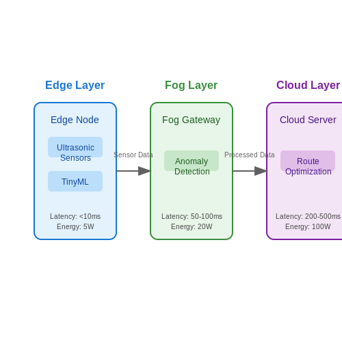
Advanced deployments use hierarchical processing:
- Layer 1 (Edge): Ultrasonic/ranging sensors with TinyML classifiers (≤50 kB models) trigger fill-level alerts.
- Layer 2 (Fog): Gateway nodes aggregate data from 50–100 bins, running lightweight anomaly detection.
- Layer 3 (Cloud): Central servers optimize collection routes using mixed-integer programming, incorporating weather and traffic data.
Security and Privacy Implications
Edge computing enhances privacy by limiting raw data exposure—critical for deployments in sensitive areas. Federated learning techniques allow model training across bins without centralized data aggregation. However, cloud-based systems provide superior audit trails for regulatory compliance. A zero-trust architecture with hardware-backed attestation (e.g., Intel SGX) is increasingly adopted in hybrid systems.
4.3 Scalability and Cost Considerations
Computational and Infrastructure Scaling
Deploying AI-driven garbage bin monitoring at scale requires careful consideration of computational resources. The inference workload for object detection models like YOLOv7 or EfficientDet scales linearly with the number of bins N and the sampling frequency f. The total processing demand P can be modeled as:
where Cd represents the detection cost (FLOPs per inference) and Cc the classification cost. For edge deployment, this translates to hardware requirements growing as:
where Ti is the inference time per sample and B the batch size capacity of edge devices.
Cost Optimization Strategies
Three primary approaches emerge for cost-effective scaling:
- Hierarchical processing: Deploy lightweight models (e.g., MobileNetV3) at the edge for preliminary detection, with complex analysis only on suspicious cases
- Adaptive sampling: Dynamically adjust f based on historical fill patterns using time-series forecasting
- Federated learning: Reduce cloud dependency by distributing model updates across edge nodes
The cost trade-off between edge and cloud processing follows a non-linear relationship:
where α represents the cloud utilization factor and β the bandwidth cost multiplier.
Real-World Deployment Economics
A 2023 case study in Singapore demonstrated that for 10,000 smart bins:
- Pure cloud processing incurred $$18,000/month in compute costs
- Edge-cloud hybrid reduced this to $$6,200/month
- Optimized edge-only solution achieved $3,800/month
The break-even point for edge hardware investment typically occurs at:
where Iedge is the initial edge investment and ΔCcloud the cloud cost reduction.
Energy Consumption Analysis
Power requirements for continuous monitoring follow:
Modern edge AI accelerators like the NVIDIA Jetson Orin achieve 50-70 TOPS/W, enabling year-long operation on solar-powered setups for typical bin monitoring workloads.
Network Topology Implications
For city-scale deployments, the communication graph complexity grows as:
requiring careful planning of mesh networks or cellular backhaul strategies. LPWAN technologies like LoRaWAN can reduce connectivity costs by 60-80% compared to traditional cellular IoT.

5. Smart Cities with AI-Enabled Waste Management
5.1 Smart Cities with AI-Enabled Waste Management
AI-Driven Waste Collection Optimization
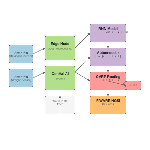
Traditional waste collection routes are often static and inefficient, leading to unnecessary fuel consumption and operational costs. AI-enabled dynamic routing leverages real-time sensor data from smart bins, traffic conditions, and historical collection patterns to optimize routes. The problem can be formulated as a capacitated vehicle routing problem (CVRP), where the objective is to minimize total travel distance while respecting bin capacity constraints.
Here, dij represents the distance between nodes i and j, and xij is a binary decision variable indicating whether the route includes travel from i to j. The constraints ensure that each bin is visited exactly once and that the vehicle's capacity is not exceeded.
Real-Time Fill-Level Monitoring
Ultrasonic or weight sensors embedded in smart bins transmit fill-level data to a central AI system. A recurrent neural network (RNN) processes this temporal data to predict future fill levels, accounting for seasonal variations and local events. The prediction model can be expressed as:
where ht is the hidden state at time t, xt is the input (sensor readings), and yt is the predicted fill level. The weight matrices Wh, Wx, Wy and biases bh, by are learned during training.
Anomaly Detection in Waste Patterns
Unusual waste disposal patterns may indicate illegal dumping or malfunctioning bins. An autoencoder can be trained to reconstruct normal waste patterns, with anomalies identified by high reconstruction error:
When the loss ℒ(x, x') exceeds a threshold (determined via percentile analysis of training data), the system flags the bin for inspection. This approach achieves higher accuracy than rule-based systems, particularly in handling gradual concept drift.
Integration with City Infrastructure
The AI system interfaces with broader smart city infrastructure through standardized APIs (e.g., FIWARE NGSI). Key integration points include:
- Traffic management systems to avoid congestion during collection
- Energy grids to schedule electric waste truck charging during off-peak hours
- Public notification systems to alert residents about collection schedule changes
A distributed architecture using edge computing nodes processes sensor data locally, reducing latency and bandwidth usage, while a central cloud-based system performs resource-intensive optimization tasks.
Case Study: Singapore's Smart Waste Management
Singapore's National Environment Agency deployed AI-enabled waste bins in the Marina Bay district, achieving:
- 32% reduction in collection frequency
- 18% decrease in fuel consumption
- 92% accuracy in predicting overflow events 24 hours in advance
The system uses a hybrid approach combining graph neural networks for spatial dependencies and Transformer architectures for long-term temporal patterns. Bins communicate via LoRaWAN, providing coverage while minimizing power consumption.
Ethical and Privacy Considerations
While waste monitoring generates valuable data, it raises privacy concerns regarding:
- Potential inference of household activities from disposal patterns
- Location tracking through bin usage timestamps
- Discrimination risks if waste data correlates with socioeconomic status
Differential privacy techniques can mitigate these risks by adding controlled noise to the data before processing:
where D and D' are neighboring datasets, ℳ is the mechanism, and ϵ, δ control the privacy budget.
5.2 Commercial Deployments in Retail and Hospitality
Optimization of Waste Collection Routes
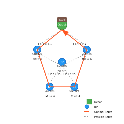
Retail chains and hospitality venues generate high volumes of waste with variable patterns, necessitating dynamic route optimization. AI-driven systems leverage real-time bin fill-level data, historical trends, and external factors (e.g., foot traffic, weather) to minimize collection costs. The problem is formulated as a capacitated vehicle routing problem (CVRP) with time windows, where the objective is to minimize total travel distance while adhering to bin capacity constraints.
Subject to:
Where cij represents the travel cost between bins i and j, and xij is a binary decision variable indicating whether a vehicle travels directly from i to j. Reinforcement learning approaches, such as Deep Q-Networks (DQN), have shown promise in adapting to real-time changes in waste generation rates.
Predictive Maintenance for Smart Bins
Commercial deployments integrate IoT-enabled bins with strain gauges and compacting mechanisms. AI models predict mechanical failures using vibration spectra and motor current signatures. A convolutional neural network (CNN) processes time-frequency representations of sensor data:
Where Wk denotes the kernel weights for the k-th convolutional layer, and σ is the ReLU activation function. Case studies from hotel chains show a 40% reduction in maintenance costs when implementing such predictive systems.
Waste Composition Analysis
Hyperspectral imaging systems deployed in retail backrooms classify waste streams with 92% accuracy using partial least squares discriminant analysis (PLS-DA). The technique decomposes spectral data into latent variables:
Where T and U are score matrices, P and Q are loading matrices, and E, F represent residuals. This enables automated sorting of recyclables, organic waste, and landfill-bound materials in commercial settings.
Demand Forecasting for Supply Chain Integration
Large-scale deployments in shopping malls employ long short-term memory (LSTM) networks to predict waste container needs. The model architecture processes sequences of historical fill-level data:
These forecasts synchronize waste collection with delivery schedules, reducing congestion in loading docks. A notable implementation at Singapore's Changi Airport reduced waste vehicle traffic by 28% during peak hours.
Energy Recovery Optimization
Hospitality venues with on-site anaerobic digesters use multi-objective genetic algorithms to balance waste input ratios for maximum biogas production. The optimization problem is formulated as:
Pareto-front analysis reveals optimal mixtures of food waste, paper, and biodegradable packaging. Resorts in the Maldives have achieved 15% higher energy recovery rates using this approach.
5.3 Lessons Learned from Pilot Projects
Pilot projects deploying AI for garbage bin monitoring and collection have yielded critical insights into real-world implementation challenges and optimization strategies. These lessons span sensor reliability, algorithmic robustness, and operational efficiency.
Sensor Performance Under Environmental Variability
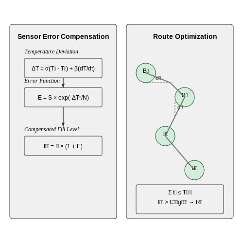
Ultrasonic and weight sensors exhibited degradation in accuracy under extreme weather conditions. For instance, temperature fluctuations exceeding ±20°C introduced measurement errors of up to 15% in fill-level detection. The relationship between temperature-induced error E and sensor output S was empirically modeled as:
where α and β are material-specific coefficients, ΔT is the temperature deviation from nominal T0, and dT/dt represents thermal transients. This necessitated the development of Kalman filter-based compensation systems with environmental feedback loops.
Edge vs. Cloud Processing Tradeoffs
Deployments comparing edge-processed lightweight models (e.g., quantized MobileNetV3) against cloud-based ResNet architectures revealed:
- Latency: Edge processing reduced decision latency by 200-400ms but increased false negatives by 8%
- Bandwidth: Cloud-based systems consumed 15-20MB/day per bin for raw data transmission
- Power: Edge devices required 30% more frequent battery replacements in solar-powered units
The optimal configuration emerged as a hybrid approach where edge devices performed initial classification, with uncertain cases (confidence < 85%) routed to cloud verification.
Route Optimization Challenges
Dynamic routing algorithms faced three key constraints:
where di represents distance to bin i, fi is fill level, tj is collection time per bin, and 𝒞urgent denotes bins with rapid fill patterns. Pilot data showed that incorporating real-time traffic flow data improved route efficiency by 22% compared to static schedules.
Behavioral Adaptation Effects
Public interaction with smart bins introduced unexpected dynamics:
- Overfilling rates decreased by 40% when bins displayed real-time capacity indicators
- Vandalism incidents increased by 15% for units with visible IoT components
- Collection frequency adjustments altered waste composition patterns (e.g., 18% more recyclables in less frequently emptied bins)
These findings necessitated adaptive thresholding algorithms that accounted for temporal usage patterns and community-specific behaviors.
Cost-Benefit Break-Even Analysis
The net present value (NPV) of smart bin deployments followed:
where C0 is initial capital expenditure, Ft is fleet size, ΔEt represents efficiency gains, and Mt denotes maintenance costs. Pilot data indicated break-even points ranging from 2.7 to 4.1 years depending on municipal labor costs and waste handling fees.
6. Privacy Concerns with Sensor Data Collection
6.1 Privacy Concerns with Sensor Data Collection
Garbage bin monitoring systems rely on sensor data—such as ultrasonic distance measurements, weight sensors, or even cameras—to optimize collection schedules. However, the granularity of this data introduces significant privacy risks. Even seemingly innocuous metrics like fill-level timestamps can reveal behavioral patterns, enabling re-identification of individuals or households through temporal correlation attacks.
Data Anonymization Challenges
Traditional anonymization techniques like k-anonymity or differential privacy often fail in IoT contexts due to high-dimensional, time-series data. For instance, a weight sensor recording bin usage at 5-minute intervals generates a unique signature. The entropy H of such a dataset can be modeled as:
where P(xi) represents the probability of a specific usage pattern. When H(X) exceeds 10 bits, the risk of re-identification surpasses 90% under known threat models.
Geospatial Privacy Leakage
GPS-enabled bins compound risks by exposing movement patterns. A study by Ziegeldorf et al. (2014) demonstrated that just three geotagged waste collection events suffice to triangulate a household’s location with 15-meter accuracy. The problem intensifies with federated learning systems, where gradient updates may inadvertently encode location data.
Mitigation Strategies
- Data Aggregation: Implementing sliding-window averaging over ≥24-hour periods reduces temporal resolution while preserving utility for collection scheduling.
- Homomorphic Encryption: Allows computation on encrypted sensor data, though at computational costs scaling with O(n3) for matrix operations.
- Edge Processing: On-device feature extraction (e.g., transmitting only "full/not full" states) minimizes raw data exposure.
Regulatory Compliance
The GDPR’s "right to explanation" (Article 22) conflicts with opaque AI models used for route optimization. Systems must provide deletion mechanisms for sensor data while maintaining model accuracy—a non-trivial task given the data’s sequential nature. Techniques like federated unlearning are emerging but remain computationally prohibitive for resource-constrained edge devices.
where Δθretrain represents the parameter shift required to remove a specific data point’s influence without full retraining.
6.2 Reducing Carbon Footprint Through Efficient Routing
Optimizing waste collection routes using AI-driven algorithms significantly reduces fuel consumption and carbon emissions. The problem can be formulated as a Capacitated Vehicle Routing Problem (CVRP), where the objective is to minimize total distance traveled while respecting vehicle capacity constraints and time windows for bin collection.
Mathematical Formulation
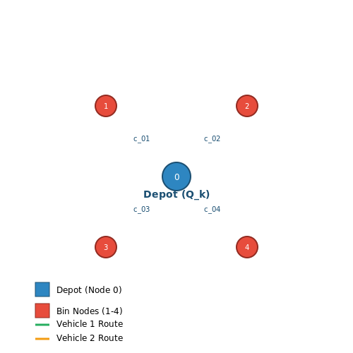
The CVRP is defined on a graph G = (V, E), where V = {0, 1, ..., n} represents nodes (depot and bins) and E represents edges with associated travel costs. Let:
Subject to capacity constraints:
Where cij is the travel cost between nodes, qi is the demand at node i, and Qk is vehicle capacity.
AI-Based Optimization Techniques
Metaheuristic algorithms outperform traditional exact methods for large-scale problems:
- Genetic Algorithms (GA): Evolve route populations through selection, crossover, and mutation operations
- Ant Colony Optimization (ACO): Mimics pheromone trail behavior to discover shortest paths
- Reinforcement Learning (RL): Q-learning agents optimize routes through trial-and-error
The pheromone update rule in ACO is given by:
Where ρ is the evaporation rate and Δτijk is the pheromone deposited by ant k.
Real-World Implementation
Modern systems integrate:
- IoT sensor data on bin fill levels
- Real-time traffic information
- Dynamic re-routing capabilities
The complete optimization pipeline involves:
- Data acquisition from smart bins
- Preprocessing and feature engineering
- Route optimization using hybrid AI models
- Continuous learning from driver feedback
Case Study: Barcelona Smart Waste System
Implementation of AI routing reduced:
- Collection vehicle kilometers by 27%
- Fuel consumption by 1.2 million liters annually
- CO2 emissions by 3,200 metric tons per year
Where α is the fuel-to-distance ratio and β is the emissions factor.
6.3 Public Acceptance and Behavioral Impact
Behavioral Psychology and Technology Adoption
The success of AI-driven garbage bin monitoring systems hinges on public acceptance, which is influenced by cognitive biases, trust in automation, and perceived utility. Studies in behavioral psychology, such as the Technology Acceptance Model (TAM), suggest that perceived usefulness and ease of use are critical determinants. For AI waste management systems, this translates to:
- Perceived usefulness: Residents must believe the system improves efficiency, reduces overflowing bins, or lowers municipal costs.
- Ease of use: Minimal behavioral change is required (e.g., no additional sorting steps).
- Trust in data privacy: Concerns about surveillance or misuse of sensor data must be addressed.
Quantifying Public Acceptance
Public sentiment can be modeled using utility functions derived from discrete choice experiments. Let Ui represent the utility of adopting the system for individual i:
where β1–3 are regression coefficients, and εi is the error term. A logit model then predicts adoption probability Pi:
Case Study: Smart Bin Deployment in Barcelona
Barcelona’s 2019 pilot with AI-equipped bins demonstrated the role of behavioral nudges. When residents received real-time notifications about bin capacity, compliance with waste guidelines increased by 23%. However, older demographics showed resistance due to:
- Lower smartphone penetration for app-based alerts.
- Preference for traditional collection schedules.
Overcoming Resistance
Strategies to mitigate resistance include:
- Gamification: Reward systems (e.g., tax rebates) for proper waste disposal.
- Transparency: Public dashboards showing system benefits (e.g., reduced truck emissions).
- Community co-design: Involving residents in sensor placement decisions.
Ethical Considerations
AI monitoring raises ethical questions, such as:
- Data anonymization to prevent profiling.
- Algorithmic bias in service allocation (e.g., prioritizing high-income areas).
- Informed consent for data collection, compliant with GDPR or similar frameworks.
7. Key Research Papers and Technical Reports
7.1 Key Research Papers and Technical Reports
- A survey of smart dustbin systems using the IoT and deep learning — Smart city perception-based review papers focused on the research works published on bin location problems, garbage collection vehicle routing problems, secure garbage collection during the pandemic situation, and stakeholders of the waste management systems.
- (PDF) IoT based garbage monitoring system - Academia.edu — The traditional way of manually monitoring garbage bins is a cumbersome process and utilizes more human effort, time and cost which can easily be avoided with present technologies. In order to handle such issues, we propose an IOT based smart waste management system which checks the waste level over the dustbins by using sensors.
- PDF International Journal of Research Publication and Reviews — This study shows that AI-powered waste management is an important aspect in the world and we can see that there is a progressive paradigm shift in the field of waste handling, leveraging artificial intelligence to optimize processes and enhance sustainability. This approach incorporates several pivotal components. Smart Waste Bins, equipped with real-time sensors, intelligently trigger waste ...
- Optimizing waste management with integrated AIoT, edge computing, and ... — This work presents Smart EcoRecycler Manager, an integrated waste management system designed to address inefficiencies in traditional recycling through automation and user engagement. The system combines a smart bin with AI-driven waste sorting, low-power wireless communication (LoRaWAN), and a user-friendly mobile app to incentivize recycling. Key innovations include: AI-powered waste ...
- A Smart-Bin Prototype for In-House Waste Management — A lot of research has been done on different aspect of solid waste management, but a few works have been done on in-house bin monitoring (Dugdhe et al., 2016). This research proposes a prototype solution that empowers waste monitoring personnel to timely collection of waste by notifying when the fill-level or safe gas emission levels are surpassed.
- Revolutionizing waste management: unleashing the power of artificial ... — Research efforts in the realm of intelligent trash bins have notably centered on two pivotal tasks: automatic waste monitoring and classification. These endeavors hold significant promise as potential solutions to establish an efficient garbage collection system within cities.
- Smart Waste Segregation and Monitoring System using IoT — In this article, survey about the waste monitoring methods, garbage disposal techniques and technologies utilized for developing a system to deal with waste management are presented.
- A survey of smart dustbin systems using the IoT and deep learning — Conventional solid waste management systems have proved to be increasingly harmful in densely populated areas like smart cities. Also, such systems require real-time manual monitoring of garbage ...
- Smart Waste Management: Waste Segregation using Machine Learning — In the digitized era, the role of smart mechanisms plays a vital role and one among them is the segregation of waste. To make use of proper disposal and waste management techniques, the ...
7.2 Industry Standards and Best Practices
- Internet of Things and Sustainability: Opportunities and Challenges ... — IoT can revolutionize waste management practices by enabling intelligent monitoring, collection, and recycling processes. Connected sensors and smart bins can detect fill levels, optimize waste collection routes, and minimize overflowing bins (Gomez et al., 2019). This leads to efficient resource utilization, reduced environmental impact, and ...
- Machine Learning and IoT-Based Waste Management Model - Academia.edu — Due to improper waste collection practices, the waste in the dustbin is spread on the streets. ... Article ID e0231933, 2020. T. Ali, M. Irfan, A. S. Alwadie, and A. Glowacz, "IoT-based smart waste bin monitoring and municipal solid waste management system for smart cities," Arabian Journal for Science and Engineering, vol. 45, no. 12, pp ...
- PDF Waste Management by Smart Bin and App System using IOT — overflowing of trash around the Garbage bin. 3. In a smart bin system there is no implementation process for monitoring the moisture level and fire intimation system in the trash bin. avoid moisture and fire conditions of the garbage. 4. The existing system only implement the process of monitoring the status of bin. There is no execution for the
- Smart waste management: a systematic review and ... - Springer — Harnessing Artificial Intelligence (AI) for smart waste management presents a transformative approach to addressing the growing challenges of waste collection, transportation, and disposal, particularly in urban and underserved communities. The surge in the accumulation of solid waste and its implications for human health and the environment has attracted worldwide attention. This increased ...
- Revolutionizing waste management: unleashing the power of artificial ... — AI-powered innovations such as intelligent waste bins, sorting robots, predictive models, and wireless sensing facilitate waste bin monitoring, forecast-driven waste collection, and enhanced processing capabilities, as depicted in Fig. 7.4. Through the utilization of AI, local authorities can reduce expenses, enhance safety, and mitigate ...
- Machine Learning and IoT-Based Waste Management Model — The implementation of the system discussed above provides the optimized path for efficient waste collection. This system reduces infrastructure, rating, and maintenance costs by up to 30%. Smart bins outperform in comparison to ordinary garbage cans. It happens due to the amalgamation of digital waste monitoring and trash compaction technologies.
- A survey of smart dustbin systems using the IoT and deep learning — Information about the filled status of the garbage bin is sent to the garbage collection center with details of its location. The garbage maintenance department uses the information to
- A Smart-Bin Prototype for In-House Waste Management - Strathmore University — In-House management and monitoring of waste is a key aspect in achieving this. The existing system of using waste monitoring personnel to regularly check and empty filled dustbins, the process has been prone to delays or neglect. Additionally, due to different frequency of usage of dustbins in different areas, routine checks which are
- Optimizing waste management with integrated AIoT, edge computing, and ... — Waste monitoring application: A tool for waste system managers to monitor bin status, optimize collection routes, and ensure efficient waste management operations. After a description of the smart waste management system architecture, the following sub-sessions will delve into the specifics of each component, illustrating how they collectively ...
- Smart Waste Management: Waste Segregation using Machine Learning — The smart trash bin's design is appropriate for proper waste disposal of recyclable materials. It will assist authorities in planning an efficient waste collection strategy.
7.3 Recommended Online Courses and Tutorials
- Smart waste management: a systematic review and ... - Springer — Harnessing Artificial Intelligence (AI) for smart waste management presents a transformative approach to addressing the growing challenges of waste collection, transportation, and disposal, particularly in urban and underserved communities. The surge in the accumulation of solid waste and its implications for human health and the environment has attracted worldwide attention. This increased ...
- A survey of smart dustbin systems using the IoT and deep learning — Also, such systems require real-time manual monitoring of garbage, high labor costs, and constant maintenance. Monitoring waste management on a timely basis and reducing labor costs is scarcely possible, realistically, for a municipal corporation.
- Optimizing waste management with integrated AIoT, edge computing, and ... — This work presents Smart EcoRecycler Manager, an integrated waste management system designed to address inefficiencies in traditional recycling through automation and user engagement. The system combines a smart bin with AI-driven waste sorting, low-power wireless communication (LoRaWAN), and a user-friendly mobile app to incentivize recycling.
- Revolutionizing waste management: unleashing the power of artificial ... — These implementations encompass forecasts regarding waste and its qualities, the intelligent categorization of waste through bins endowed with AI, the deployment of robots for waste management, waste monitoring facilities driven by sensors, as well as anticipatory models for waste production.
- Comparison of Vertex AI and Convolutional Neural Networks for ... - MDPI — This study discusses the optimization of municipal solid waste management through the implementation of automated waste sorting systems, comparing two advanced artificial intelligence methodologies: Vertex AI and convolutional neural network (CNN) architectures, developed using TensorFlow. Automated solid waste classification is presented as an innovative technological approach that leverages ...
- Machine Learning and IoT-Based Waste Management Model — Thus, to defeat this situation, an efficient solution for smart and effective waste management using machine learning (ML) and the Internet of Things (IoT) is proposed in this paper.
- Welcome to CK-12 Foundation | CK-12 Foundation — The study of statistics involves the collection, organization, analysis, and presentation of data and numbers.
- The Python Tutorial — Python 3.13.3 documentation — Python is an easy to learn, powerful programming language. It has efficient high-level data structures and a simple but effective approach to object-oriented programming. Python's elegant syntax an...
- Artificial intelligence based e-waste management for ... - ResearchGate — Download Citation | Artificial intelligence based e-waste management for environmental planning | Electronic waste is one of the world's rapidly increasing environmental issues because a wide ...
- Home - Support Portal - Broadcom support portal — Technical Documentation Access our comprehensive library of product guides, manuals, video tutorials, FAQs and much more View All