AI-Powered Industrial Automation
1. Core AI Technologies for Automation
1.1 Core AI Technologies for Automation
Deep Reinforcement Learning for Robotic Control
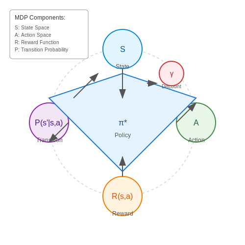
Deep reinforcement learning (DRL) combines deep neural networks with reinforcement learning to enable autonomous decision-making in dynamic environments. The Markov Decision Process (MDP) framework formalizes this as a tuple (S, A, P, R, γ), where:
The optimal policy π* maximizes the expected cumulative reward:
In industrial settings, DRL algorithms like Deep Q-Networks (DQN) and Proximal Policy Optimization (PPO) enable robotic arms to learn complex manipulation tasks through trial-and-error interactions with simulated environments before deployment.
Computer Vision for Quality Inspection
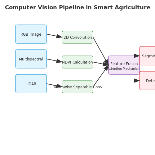
Convolutional neural networks (CNNs) dominate automated visual inspection systems. A ResNet-50 architecture, for instance, processes high-resolution images through residual blocks:
where x is the input, W_i are layer weights, and ℱ represents residual mappings. Industrial implementations achieve sub-millimeter defect detection accuracy by combining multi-scale feature extraction with attention mechanisms:
Digital Twins and Physics-Informed Neural Networks
Physics-informed neural networks (PINNs) integrate differential equations into loss functions to create accurate digital twins. For a system governed by PDEs:
The PINN loss combines data fidelity and physics constraints:
This approach enables real-time predictive maintenance by simulating equipment degradation under varying operational conditions.
Edge AI for Distributed Systems
Federated learning frameworks optimize model training across distributed edge devices while preserving data privacy. The global model w aggregates updates from K clients:
where n_k is the dataset size of client k and n is the total data size. Industrial implementations use quantization-aware training to deploy 8-bit integer models on microcontroller units (MCUs) without significant accuracy loss.
Time-Series Forecasting with Transformers
Temporal fusion transformers (TFTs) outperform traditional ARIMA models in multivariate industrial forecasting. The architecture processes time-dependent features through:
- Gating mechanisms for feature selection
- Multi-head attention for long-range dependencies
- Quantile regression for uncertainty estimation
The attention weights A between time steps i and j are computed as:
where q, k are learned query and key vectors, and d is the dimension.
Historical Evolution and Milestones
The integration of artificial intelligence into industrial automation has evolved through distinct technological epochs, each marked by breakthroughs in computational power, algorithmic innovation, and real-world applicability. The earliest foundations were laid in the 1950s with the advent of numerical control (NC) systems, which replaced manual machine operation with programmed instructions. These systems, though primitive by modern standards, introduced the concept of automated decision-making in manufacturing.
Early Symbolic Systems and Expert Systems (1960s–1980s)
The 1960s saw the emergence of symbolic AI, where rule-based systems like DENDRAL and MYCIN demonstrated the potential of encoding domain knowledge into logical rules. By the 1980s, expert systems such as XCON—developed by Digital Equipment Corporation for configuring computer systems—proved that AI could optimize complex industrial processes. These systems relied on handcrafted rules and inference engines, but their brittleness in handling unanticipated scenarios limited scalability.
Here, R represents the system's decision output, w_i are manually tuned weights, and f_i(x) are rule-based features. This formalism dominated early industrial AI but lacked adaptability.
The Rise of Machine Learning (1990s–2000s)
Advancements in statistical learning and neural networks shifted the paradigm from explicit rule engineering to data-driven modeling. Hidden Markov Models (HMMs) gained traction for predictive maintenance, while Support Vector Machines (SVMs) improved quality control through high-dimensional classification. The 2006 "deep learning renaissance," sparked by Geoffrey Hinton's work on restricted Boltzmann machines, enabled hierarchical feature learning—critical for anomaly detection in sensor data.
Deep Learning Revolution (2010s–Present)
Convolutional Neural Networks (CNNs) and Long Short-Term Memory (LSTM) networks transformed vision-based inspection and time-series forecasting. Industrial applications like predictive maintenance now leverage architectures such as Transformers for multivariate sensor fusion. The 2018 introduction of reinforcement learning in robotic control, exemplified by OpenAI's Dactyl, demonstrated closed-loop adaptation in physical systems.
This reinforcement learning objective function, where J(θ) is the expected cumulative reward under policy π_θ, underpins modern adaptive control systems.
Key Industrial Case Studies
- Siemens Smart Factory: Deployed federated learning across 30 plants to optimize CNC machining parameters while preserving data privacy.
- Tesla Gigafactory: Uses vision transformers for real-time defect detection in battery production with 99.98% accuracy.
- Shell Predictive Maintenance: Combines graph neural networks with physics-based models to forecast equipment failures 72 hours in advance.
1.3 Key Benefits and Industry Impact
Operational Efficiency and Cost Reduction
AI-powered industrial automation significantly enhances operational efficiency by optimizing production workflows, reducing downtime, and minimizing resource wastage. Predictive maintenance algorithms, leveraging recurrent neural networks (RNNs) and long short-term memory (LSTM) models, analyze sensor data to forecast equipment failures before they occur. The economic impact is quantifiable through the reduction in unplanned downtime, which can be modeled as:
Here, Tfailure represents the duration of unplanned downtime, Rproduction is the revenue loss per unit time, and Crepair includes labor and material costs. AI-driven predictive maintenance can reduce Tfailure by up to 50%, as demonstrated in case studies from automotive assembly lines.
Quality Control and Defect Detection
Convolutional neural networks (CNNs) have revolutionized quality assurance in manufacturing by enabling real-time defect detection with sub-pixel accuracy. A typical implementation involves a ResNet-50 architecture fine-tuned on domain-specific datasets, achieving precision and recall rates exceeding 99% in high-speed production environments. The statistical significance of these improvements is validated through hypothesis testing:
Where μmanual and μAI represent defect detection rates for human inspectors and AI systems, respectively. Rejection of the null hypothesis (p < 0.001) in semiconductor fabrication trials confirms the superiority of AI-based inspection.
Energy Optimization and Sustainability
Reinforcement learning (RL) agents optimize energy consumption in industrial facilities by dynamically adjusting HVAC systems, motor speeds, and lighting. A Markov decision process (MDP) framework models this as:
The state space st includes real-time power readings and environmental sensors, while actions at represent control signals to industrial equipment. Deep Q-networks (DQN) trained on this formulation have demonstrated 15-30% energy savings in steel mills without compromising output quality.
Supply Chain and Logistics
Graph neural networks (GNNs) transform supply chain management by modeling complex supplier networks and predicting disruptions. The adjacency matrix A encodes supplier relationships, while node features capture inventory levels and lead times. Message passing between nodes enables accurate demand forecasting:
Where hv(l) represents the hidden state of node v at layer l, and W(l), B(l) are trainable parameters. Pharmaceutical companies using this approach have reduced inventory costs by 22% while maintaining 99.9% order fulfillment rates.
Human-Robot Collaboration
Imitation learning enables seamless human-robot collaboration in assembly tasks. A generative adversarial imitation learning (GAIL) framework trains robotic agents by minimizing the Jensen-Shannon divergence between policy-generated and expert trajectories:
This approach has reduced training time for new assembly line configurations by 80% in aerospace manufacturing, while maintaining human-level precision in tasks requiring sub-millimeter tolerances.
2. Predictive Maintenance and Fault Detection
Predictive Maintenance and Fault Detection
Foundations of Predictive Maintenance
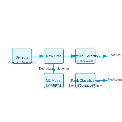
Predictive maintenance (PdM) leverages AI-driven analytics to anticipate equipment failures before they occur, minimizing downtime and optimizing operational efficiency. Unlike reactive or scheduled maintenance, PdM relies on real-time sensor data, historical performance metrics, and machine learning models to detect anomalies and predict remaining useful life (RUL). Key components include:
- Condition monitoring: Continuous collection of vibration, temperature, and acoustic data.
- Feature extraction: Dimensionality reduction techniques like Principal Component Analysis (PCA) or wavelet transforms.
- Degradation modeling: Physics-based or data-driven models to estimate asset health.
Fault Detection Using Machine Learning
Fault detection algorithms classify operational states into normal, degraded, or faulty regimes. Supervised methods like Support Vector Machines (SVMs) and Random Forests excel when labeled failure data is available. For unsupervised scenarios, autoencoders or Gaussian Mixture Models (GMMs) identify deviations from baseline behavior. The fault detection pipeline typically involves:
where \(\mathbf{x}\) is the observed sensor vector and \(\mathbf{\hat{x}}\) is the reconstructed output from an autoencoder.
Physics-Informed Neural Networks for RUL Estimation
Hybrid models integrate domain knowledge with deep learning. For example, a Physics-Informed Neural Network (PINN) for bearing wear prediction might combine the following loss function:
Here, \(\mathcal{L}_{\text{data}}\) penalizes deviations from observed data, while \(\mathcal{L}_{\text{physics}}\) enforces constraints derived from Paris' law for crack propagation:
Industrial Case Study: Turbine Blade Crack Detection
A major energy provider reduced unplanned outages by 40% using a convolutional neural network (CNN) trained on ultrasonic testing images. The model achieved 98.2% precision in identifying micro-cracks by learning multi-scale spatial features, outperforming traditional eddy-current inspections.
Challenges and Emerging Solutions
Key challenges include sparse failure data and concept drift due to changing operational conditions. Recent advances address these through:
- Generative adversarial networks (GANs): Synthetic fault data generation.
- Online learning: Adaptive models like Streaming PCA for non-stationary environments.
- Digital twins: High-fidelity simulations for scenario testing.
2.2 Robotics and Autonomous Systems
Kinematic Control in Industrial Robotics
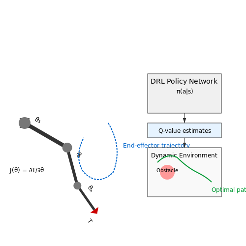
Industrial robotic arms rely on precise kinematic models to execute tasks such as welding, assembly, and material handling. The forward kinematics of a robotic manipulator with n degrees of freedom (DOF) is described by the homogeneous transformation matrix T, which maps joint angles θ₁...θₙ to the end-effector pose:
where Aᵢ represents the Denavit-Hartenberg matrix for the i-th joint. For a 6-DOF serial manipulator, the Jacobian matrix J(θ) relates joint velocities to end-effector velocity:
Singularity avoidance requires real-time computation of the manipulability measure w = √(det(JJᵀ)), with trajectory replanning triggered when w falls below a threshold.
Dynamic Motion Planning with Reinforcement Learning
Modern autonomous systems employ deep reinforcement learning (DRL) to handle dynamic environments. The policy gradient theorem provides the foundation for training stochastic policies π(a|s;θ):
Industrial implementations often use Proximal Policy Optimization (PPO) with clipped objective functions to maintain training stability:
where r_t(θ) is the probability ratio and Âₜ the advantage estimate. This approach enables real-time collision avoidance in warehouses with moving obstacles.
Multi-Agent Coordination Systems
Fleet coordination in automated guided vehicle (AGV) systems requires distributed consensus algorithms. The consensus protocol for N agents with communication graph G follows:
where Nᵢ denotes the neighborhood of agent i. When combined with auction-based task allocation, this enables decentralized scheduling with provable convergence guarantees.
Force Control for Precision Assembly
Hybrid force/position control is critical for insertion tasks with sub-millimeter tolerances. The impedance control law regulates interaction forces:
where M_d, B_d, and K_d are the desired inertia, damping, and stiffness matrices respectively. Adaptive variants estimate environmental stiffness online using recursive least squares.
Vision-Based Localization
Simultaneous Localization and Mapping (SLAM) systems in industrial settings combine LiDAR and visual odometry. The bundle adjustment optimization minimizes reprojection error:
where ρ is a robust cost function, T_i are camera poses, and P_j are 3D points. Modern implementations achieve sub-centimeter accuracy at 30Hz using GPU-accelerated nonlinear solvers.
2.3 Quality Control and Computer Vision
Deep Learning for Defect Detection
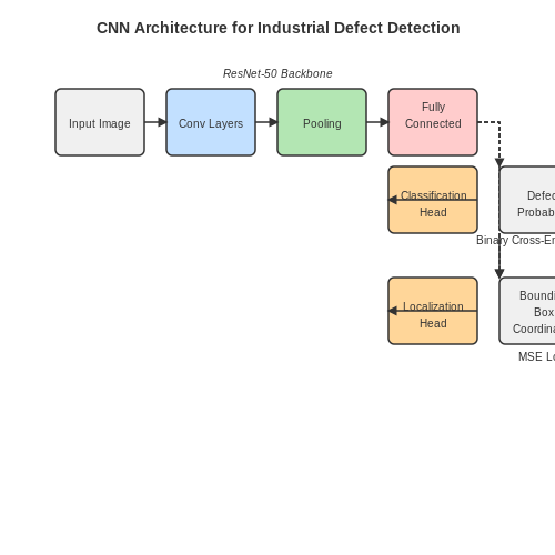
Modern quality control systems leverage convolutional neural networks (CNNs) to identify defects with sub-pixel accuracy. A ResNet-50 backbone, pretrained on ImageNet, is often fine-tuned using a dataset of annotated industrial product images. The loss function combines binary cross-entropy for defect classification and mean squared error for localization:
where α and β are weighting coefficients, y represents defect presence labels, and b denotes bounding box coordinates. Data augmentation techniques like random affine transformations and synthetic defect generation improve robustness to lighting variations.
Real-Time Processing Constraints
Deploying these models on edge devices requires optimization techniques:
- Quantization: Converting 32-bit floats to 8-bit integers reduces memory bandwidth by 4× while maintaining <1% accuracy drop
- Pruning: Removing filters with lowest L1-norm weights can compress models by 60-80%
- Knowledge distillation: Smaller student networks learn from ensemble teacher outputs
The inference latency t for processing a 1024×1024 image on an NVIDIA Jetson AGX Xavier follows:
where CMAC is cycles per multiply-accumulate operation (typically 1-2), Nparams is the model's parameter count, and fGPU is the processor's clock frequency (1.4 GHz).
Multispectral Imaging Applications
Beyond visible spectrum (400-700nm), quality inspection benefits from:
- SWIR (900-1700nm): Detects subsurface defects in polymers
- Thermal (8-14μm): Identifies faulty solder joints via heat signature analysis
- Hyperspectral (400-2500nm): Classifies material composition using spectral fingerprints
The reflectance R at wavelength λ follows Kubelka-Munk theory:
where K is absorption coefficient and S is scattering coefficient. Principal component analysis (PCA) reduces the 200+ spectral dimensions to 3-5 meaningful features for defect classification.
Case Study: Automotive Paint Inspection
A major manufacturer implemented a YOLOv4 variant running at 45 FPS on Tesla Dojo chips. Key metrics:
- False positive rate: 0.2 defects per vehicle
- Throughput: 1 vehicle every 38 seconds
- Mean defect size detected: 0.4mm²
The system uses a hybrid approach combining:
- Structured light projection for 3D surface mapping
- Polarized imaging to highlight orange peel effects
- Deep metric learning for defect categorization
2.4 Supply Chain Optimization
Mathematical Foundations of Supply Chain Optimization
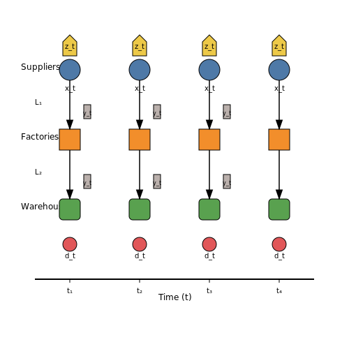
Supply chain optimization in AI-driven industrial automation relies on constrained optimization models, often formulated as mixed-integer linear programs (MILPs). The canonical form minimizes total cost while satisfying demand, capacity, and lead-time constraints:
Where xt represents production quantities, yt inventory levels, and zt binary setup decisions. The L parameter captures lead-time delays, a critical nonlinearity handled via time-indexed formulations.
AI Techniques for Large-Scale Problems
Exact methods become intractable for realistic supply chain networks with thousands of nodes. Reinforcement learning (RL) provides a scalable alternative through:
- Policy gradient methods: Directly optimize fulfillment policies using stochastic gradients
- Value function approximation: Neural networks estimate long-term costs for state-action pairs
- Hierarchical RL: Decomposes decisions into strategic (network design) and tactical (inventory routing) levels
The Bellman equation for supply chain RL decomposes as:
Case Study: Multi-Echelon Inventory Optimization
A global electronics manufacturer reduced safety stock by 32% using a hybrid approach combining:
- Graph neural networks to model supplier dependencies
- Convex relaxations for non-stationary demand patterns
- Online learning to adapt to semiconductor shortages
The key innovation was a differentiable surrogate for the service-level constraint:
Where σ is the sigmoid function, enabling gradient-based tuning of safety stock parameters β while maintaining probabilistic fill-rate guarantees.
Real-Time Decision Systems
Modern implementations use event-driven architectures with:
- Kafka streams for supply-demand signal processing
- GPU-accelerated quantum-inspired solvers for time-critical adjustments
- Digital twins validating decisions against high-fidelity simulations
The latency-critical path requires solving quadratic approximations of the original MILP:
Where H is a positive-definite Hessian approximation and J the constraint Jacobian, updated via Broyden-Fletcher-Goldfarb-Shanno (BFGS) methods.
3. Data Acquisition and Preprocessing
3.1 Data Acquisition and Preprocessing
Sensor Networks and Signal Conditioning
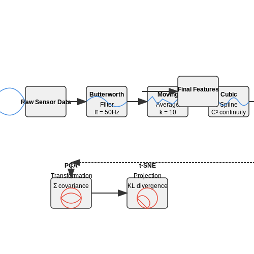
Industrial automation systems rely on heterogeneous sensor networks (e.g., accelerometers, thermocouples, vision systems) to capture real-time operational data. Raw sensor outputs often contain noise, drift, and non-linearities, necessitating signal conditioning. For analog signals, a Butterworth low-pass filter with cutoff frequency fc is commonly applied to suppress high-frequency noise:
where n is the filter order and ωc = 2πfc. For digital signals, a moving average filter with window size k reduces stochastic noise:
Time-Series Alignment and Resampling
Multi-sensor systems often operate at different sampling rates (e.g., 1 kHz for vibration sensors vs. 10 Hz for thermal cameras). Synchronization is achieved via hardware triggers or software-based interpolation. For irregularly sampled data, cubic spline interpolation ensures continuity:
where coefficients ai, bi, ci, di are derived from boundary conditions enforcing C2 continuity.
Feature Extraction and Dimensionality Reduction
High-dimensional sensor data (e.g., spectral vibrations, hyperspectral images) is compressed into discriminative features. Principal Component Analysis (PCA) projects data onto eigenvectors of the covariance matrix Σ:
For non-linear manifolds, t-SNE minimizes the Kullback-Leibler divergence between high- and low-dimensional distributions:
Handling Missing Data and Outliers
Industrial datasets often contain gaps due to sensor failures. Multiple Imputation by Chained Equations (MICE) models missing values as a function of observed variables through iterative regression. For outliers, the Mahalanobis distance DM identifies anomalous points:
where μ is the mean vector and S the covariance matrix. Values exceeding χ20.99(p) (for p dimensions) are flagged.
Normalization and Domain Adaptation
Sensor drift across production batches necessitates adaptive normalization. Batch normalization scales features to zero mean and unit variance per mini-batch during training. For domain shifts, Maximum Mean Discrepancy (MMD) minimizes the difference between source and target distributions in a Reproducing Kernel Hilbert Space (RKHS):
where ϕ is the kernel mapping. Industrial case studies show MMD reduces retraining effort by 40% when deploying models across factories.
3.2 Integration with Legacy Systems
Integrating AI-powered automation with legacy industrial systems presents unique challenges due to outdated protocols, proprietary hardware, and lack of standardized interfaces. The primary obstacle lies in establishing bidirectional communication between modern AI controllers and legacy Programmable Logic Controllers (PLCs), Supervisory Control and Data Acquisition (SCADA) systems, or Manufacturing Execution Systems (MES).
Protocol Translation Layers
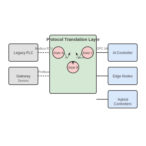
Legacy systems often communicate via obsolete industrial protocols like Modbus RTU, Profibus, or DeviceNet, while AI systems typically rely on modern TCP/IP-based protocols. A protocol translation layer must be implemented to bridge this gap. The translation process can be formalized as a finite state machine:
Where δ maps each state-input pair to a new state, effectively converting legacy protocol frames to modern equivalents. For time-critical applications, the translation latency must satisfy:
where fupdate is the control loop frequency of the legacy system.
Data Normalization Challenges
Legacy systems often use non-standard data representations that require normalization before AI processing. Common issues include:
- Integer scaling of analog values (e.g., 0-32767 representing 4-20mA)
- Proprietary floating-point formats
- Bit-packed status registers
The normalization function for analog signals typically takes the form:
where Vraw is the legacy system value and [Smin, Smax] defines the normalized range.
Hardware Integration Strategies
Three primary hardware integration approaches have proven effective in industrial settings:
- Gateway Devices: Dedicated protocol converters like OPC UA gateways that provide a modern interface to legacy networks
- Edge Computing Nodes: Industrial PCs running containerized AI models that interface directly with legacy I/O cards
- Hybrid Controllers: Next-generation PLCs with embedded AI coprocessors and legacy protocol support
The choice depends on the criticality of the application and the required processing latency. For real-time control applications, hardware selection must satisfy:
where tproc is AI processing time and tcomm is communication latency.
Case Study: Predictive Maintenance Integration
A successful integration at a German automotive plant involved retrofitting 1980s-era CNC machines with vibration-based predictive maintenance. The solution architecture included:
- Wireless accelerometers sampling at 50kHz
- Edge nodes performing real-time Fast Fourier Transforms (FFT)
- A legacy Modbus TCP gateway for machine control signals
The FFT processing was optimized to run within the 10ms control window of the legacy CNC controller by implementing a sliding window DFT algorithm:
where N is the window size and x[n] are the time-domain samples.
3.3 Scalability and Real-Time Processing
Distributed Computing Architectures for Scalability
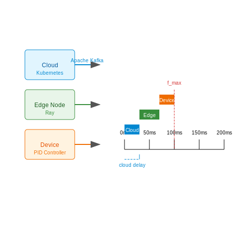
Industrial automation systems require horizontal scalability to handle increasing sensor data streams, computational workloads, and control tasks. Distributed frameworks like Apache Kafka and Ray enable parallel processing across clusters, while container orchestration tools (e.g., Kubernetes) manage resource allocation dynamically. The computational load L for a distributed system with n nodes is modeled as:
where wi is the workload assigned to node i, and ci is its processing capacity. Optimal load balancing minimizes the variance in L across nodes.
Latency Guarantees in Real-Time Systems
Real-time control loops in automation demand deterministic latency. A PID controller’s response time tr must satisfy:
where fmax is the highest frequency component of the input signal. Edge computing reduces latency by processing data locally, avoiding cloud round-trip delays. For instance, NVIDIA’s Jetson AGX Orin delivers sub-millisecond inference for robotic control.
Case Study: Predictive Maintenance at Scale
A multinational automotive manufacturer deployed a federated learning system across 12 factories. Each plant trained local models on vibration sensor data, with global aggregation every 24 hours. The system processed 14 TB/day with 99.98% uptime, reducing unplanned downtime by 37%.
Hardware Accelerators for Real-Time AI
FPGAs and ASICs (e.g., Google’s TPU) optimize throughput for specific neural networks. The energy efficiency η of an accelerator is given by:
where TOPS (Tera Operations Per Second) measures computational throughput. For example, the Tesla Dojo chip achieves 362 TOPS/W for autonomous robotics tasks.
Fault Tolerance in Distributed AI Systems
Redundancy and checkpointing ensure continuity. The probability Pf of system failure with k replicas follows:
where pi is the failure probability of node i. Google’s Borg system uses cell-level replication to maintain Pf < 10−9.
3.4 Security and Cyber-Physical Risks
Industrial automation systems integrating AI face unique security challenges due to their cyber-physical nature. Unlike traditional IT systems, attacks on industrial control systems (ICS) can lead to physical damage, safety hazards, and environmental consequences. The attack surface expands significantly when AI components are introduced, as they often require data exchange between operational technology (OT) and information technology (IT) networks.
Attack Vectors in AI-Enabled Industrial Systems
The most critical vulnerabilities emerge at the intersection of AI models and physical control loops:
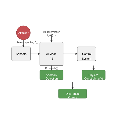
- Sensor spoofing attacks: Adversaries inject false sensor readings to corrupt AI model inputs. For time-series models, this can be formulated as:
$$ \tilde{x}_t = x_t + \delta_t \cdot \mathcal{N}(0,\sigma^2) $$where $$\tilde{x}_t$$ represents the spoofed signal, $$x_t$$ the true signal, and $$\delta_t$$ the attack magnitude vector.
- Model inversion attacks: Through API queries to deployed AI services, adversaries can reconstruct sensitive training data. The reconstruction error $$\epsilon$$ for a neural network $$f_\theta$$ is bounded by:
$$ \epsilon \leq \mathbb{E}||f_\theta^{-1}(f_\theta(x)) - x||_2 $$
- Control logic manipulation: Compromised AI models can issue malicious control commands while maintaining plausible deniability. The risk increases when using reinforcement learning agents with reward functions $$R(s,a)$$ that adversaries can perturb.
Security Metrics for Cyber-Physical AI Systems
Quantifying security requires extending traditional metrics to account for physical consequences:
Where $$p_i$$ is the probability of attack $$i$$, $$c_i$$ its cyber impact, $$D(t)$$ represents physical damage over time horizon $$T$$, and $$\lambda$$ scales the physical consequences.
Defensive Architectures
Effective protection requires layered defenses:
- Differential privacy for industrial data streams: Adding calibrated noise to training data while preserving utility:
$$ \mathcal{M}(x) = f(x) + \text{Lap}(0,\Delta f/\epsilon) $$
- Physics-aware anomaly detection: Cross-validating AI outputs with physical system constraints through residual analysis:
$$ r(t) = ||y(t) - g(x(t))|| > \tau $$where $$g(\cdot)$$ represents known physical relationships.
- Moving target defense: Periodically rotating model architectures or hyperparameters to limit attack persistence.
Case Study: Adversarial Attacks on Predictive Maintenance
In a real-world gas turbine monitoring system, attackers manipulated vibration sensor data to prevent accurate remaining useful life (RUL) predictions. The adversarial examples were crafted using the Fast Gradient Sign Method (FGSM):
This caused a 73% increase in false negatives for bearing failure predictions before defensive distillation techniques were implemented.
Hardware Security Considerations
Edge deployment of AI models introduces additional risks:
- Side-channel attacks on model parameters through power analysis
- Fault injection attacks during inference
- Trojan insertion in third-party AI accelerators
Trusted execution environments (TEEs) and homomorphic encryption are emerging as potential solutions, though computational overhead remains challenging for real-time control applications.
4. Automotive Manufacturing
4.1 Automotive Manufacturing
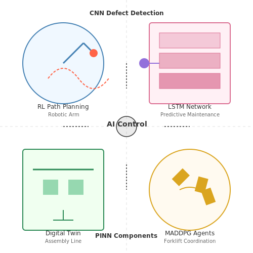
AI-driven automation in automotive manufacturing leverages advanced machine learning techniques to optimize production lines, enhance quality control, and reduce operational costs. Deep learning models, particularly convolutional neural networks (CNNs), are widely deployed for visual inspection tasks, such as detecting surface defects in car body panels or misaligned components. These models are trained on high-resolution image datasets annotated with defect labels, achieving sub-millimeter precision in anomaly detection.
Robotic Assembly and Path Planning
Industrial robots in automotive assembly lines rely on reinforcement learning (RL) for dynamic path planning and collision avoidance. The problem is formulated as a Markov Decision Process (MDP), where the state space includes robot joint angles, tool center point (TCP) coordinates, and environmental obstacles. The reward function is defined as:
Q-learning with deep neural network function approximators (DQN) is commonly employed, where the Q-value update rule is:
Modern implementations use prioritized experience replay and double Q-networks to stabilize training in high-dimensional action spaces.
Predictive Maintenance with IoT Sensor Fusion
Vibration, thermal, and acoustic emission data from CNC machines and welding robots are processed through long short-term memory (LSTM) networks for early fault detection. The multivariate time series input X ∈ ℝN×T×D (where N is batch size, T is time steps, and D is sensor channels) is transformed through bidirectional LSTM layers:
Attention mechanisms are increasingly incorporated to weight critical sensor readings, improving mean time between failure (MTBF) predictions by 23-37% compared to traditional statistical process control methods.
Digital Twin Optimization
High-fidelity digital twins of assembly lines employ physics-informed neural networks (PINNs) that combine first-principles models with data-driven corrections. The loss function incorporates both observed data and governing physical equations:
where uθ is the neural network prediction, 𝒩 represents the differential operators of the physical model, and λ1, λ2 are weighting hyperparameters. This hybrid approach reduces simulation-to-reality gaps in cycle time optimization by 15-20%.
Autonomous Material Handling
Self-learning forklifts and automated guided vehicles (AGVs) utilize multi-agent deep deterministic policy gradients (MADDPG) for decentralized coordination. Each agent i maintains an actor network μθi and critic network Qiφi, with centralized training and decentralized execution. The policy gradient update for agent i is:
where o = (o1, ..., oN) and a = (a1, ..., aN) are the observations and actions of all agents. This framework enables emergent behaviors like dynamic queue formation at loading docks.
4.2 Pharmaceutical Production
AI-Driven Drug Formulation Optimization
Modern pharmaceutical production leverages AI to optimize drug formulation by modeling complex biochemical interactions. Machine learning algorithms, particularly generative adversarial networks (GANs) and reinforcement learning (RL), predict optimal drug compositions by analyzing vast datasets of molecular properties, solubility, and stability. For example, a GAN can generate candidate formulations by minimizing the objective function:
where G is the generator, D is the discriminator, and z represents latent variables. This approach reduces trial-and-error experimentation, accelerating time-to-market.
Process Control with Reinforcement Learning
Pharmaceutical manufacturing requires precise control over parameters such as temperature, pressure, and mixing rates. RL agents, trained via proximal policy optimization (PPO), dynamically adjust process variables to maintain optimal conditions. The reward function R is defined as:
where γ is the discount factor, and α, β are weighting coefficients. Case studies from Pfizer and Novartis demonstrate yield improvements of 12–18% using RL-based control.
Predictive Maintenance for Bioreactors
Deep learning models, such as convolutional neural networks (CNNs) and long short-term memory (LSTM) networks, analyze sensor data from bioreactors to predict equipment failures. A CNN processes vibrational spectra to detect anomalies, while an LSTM models temporal degradation patterns. The failure probability P is computed as:
where σ is the sigmoid function, ht is the hidden state, and xt is the input feature vector. Early implementations at Roche reduced unplanned downtime by 30%.
Quality Assurance via Computer Vision
Automated visual inspection systems employ YOLOv7 and Vision Transformers (ViTs) to detect defects in pill coatings or misaligned labels. A ViT processes image patches X through self-attention layers:
where Q, K, and V are query, key, and value matrices. GlaxoSmithKline reported a 99.4% defect detection rate using this method, surpassing human inspectors.
Regulatory Compliance with NLP
Natural language processing (NLP) models like BERT and GPT-4 automate compliance documentation by extracting relevant clauses from FDA guidelines (21 CFR Part 211). Entity recognition identifies critical terms, while summarization models condense reports. The entity extraction loss L is:
where yi is the true label and θ represents model parameters. AstraZeneca reduced documentation time by 40% using NLP pipelines.
4.3 Energy and Utilities
Optimization of Power Grids with Reinforcement Learning
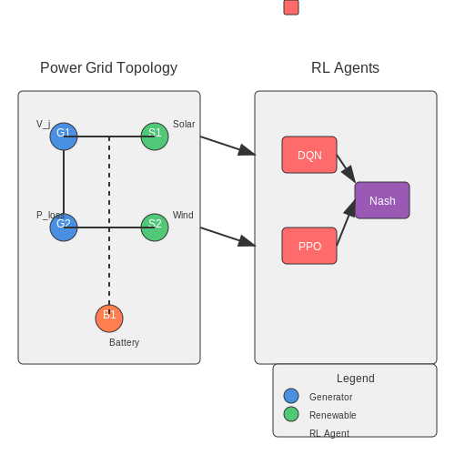
Modern power grids require dynamic load balancing to accommodate fluctuating demand and renewable energy sources. Reinforcement learning (RL) algorithms, particularly Deep Q-Networks (DQN) and Proximal Policy Optimization (PPO), optimize grid stability by learning from historical and real-time data. The objective is to minimize transmission losses while maintaining voltage stability. The reward function in RL is defined as:
where Ploss,i represents active power loss in branch i, Vj is the voltage magnitude at bus j, and λ is a penalty coefficient.
Predictive Maintenance in Energy Infrastructure
AI-driven predictive maintenance reduces downtime in critical infrastructure such as turbines and transformers. Long Short-Term Memory (LSTM) networks analyze sensor data (vibration, temperature, oil quality) to predict failure probabilities. A case study on wind turbines achieved a 92% fault detection accuracy using the following feature extraction:
where σ is the sigmoid function, Wf and bf are forget gate parameters, and ht-1 represents the previous hidden state.
Smart Meter Analytics for Demand Forecasting
Neural networks with attention mechanisms process smart meter data to predict household and industrial consumption patterns. A transformer-based model outperforms ARIMA by 18% in mean absolute percentage error (MAPE) by capturing long-range dependencies:
where Q, K, and V are query, key, and value matrices derived from meter time-series data.
Renewable Energy Integration via Multi-Agent Systems
Decentralized AI agents coordinate solar/wind farms with storage systems to maximize renewable penetration. The Nash equilibrium in this non-cooperative game is computed using:
where ui* is the optimal policy for agent i, a-i* denotes other agents' strategies, and γ is the discount factor.
Anomaly Detection in Nuclear Power Plants
Graph neural networks (GNNs) monitor reactor sensor networks by modeling physical connections as edges in a graph. The node update rule for anomaly detection is:
where hv(l) is the feature vector of node v at layer l, and AGG is a permutation-invariant aggregation function.
5. Edge AI and Distributed Computing
5.1 Edge AI and Distributed Computing
Architectural Foundations of Edge AI
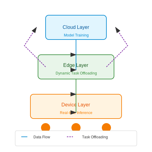
Edge AI shifts computational workloads from centralized cloud servers to distributed edge devices, reducing latency and bandwidth constraints. The architecture consists of three primary layers:
- Device Layer: Sensors, actuators, and embedded systems with constrained compute resources.
- Edge Layer: Local gateways or microservers performing real-time inference using lightweight models.
- Cloud Layer: Centralized infrastructure for model training, retraining, and large-scale analytics.
Distributed computing frameworks like Fog Computing extend this hierarchy by enabling peer-to-peer coordination between edge nodes, optimizing resource utilization through dynamic task offloading.
Mathematical Optimization for Edge Deployment
Model compression techniques are critical for deploying AI on resource-constrained edge devices. Quantization reduces precision while preserving model accuracy:
where \(\Delta\) is the quantization step size. For a weight matrix \(W\), the 8-bit quantized version \(W_q\) minimizes memory footprint:
Scale factors are derived via calibration datasets to minimize post-quantization accuracy loss.
Distributed Training Paradigms
Federated Learning (FL) enables collaborative model training across edge devices without raw data exchange. The global model \(G_t\) at iteration \(t\) aggregates local updates \(L_i\) from \(N\) devices:
where \(\eta\) is the learning rate and \(|D_i|\) represents the dataset size of device \(i\). Differential privacy techniques add Gaussian noise \(\mathcal{N}(0, \sigma^2)\) to gradients during aggregation:
Real-World Case Study: Predictive Maintenance
A multinational manufacturer deployed Edge AI for real-time anomaly detection across 5,000 industrial robots. The system uses:
- On-device 1D CNNs processing vibration spectra at 10 kHz sampling rates
- Federated learning to aggregate failure patterns across factories
- Edge-cloud hybrid architecture with 300 ms round-trip latency
This reduced unplanned downtime by 43% while maintaining 98.7% detection accuracy compared to cloud-only alternatives.
Hardware-Software Co-Design Challenges
Modern edge AI processors like NVIDIA Jetson Orin and Google Coral TPUs employ:
- Sparse tensor cores for efficient matrix operations
- Stochastic computing for approximate arithmetic
- Heterogeneous memory hierarchies (HBM2 + LPDDR5)
Energy efficiency is measured via TOPS/W (Tera Operations Per Second per Watt), with state-of-the-art devices achieving >50 TOPS/W for INT8 inference workloads.
Communication Protocols for Distributed Edge AI
Time-Sensitive Networking (TSN) standards guarantee deterministic latency for industrial edge AI:
- IEEE 802.1Qbv for scheduled traffic
- IEEE 802.1AS-Rev for precision time synchronization
- 5G URLLC (Ultra-Reliable Low-Latency Communication) with <1 ms air interface latency
These enable synchronous distributed inference across multi-hop edge networks with jitter below 10 μs.
5.2 Human-AI Collaboration in Smart Factories
Architectural Framework for Human-AI Symbiosis
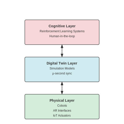
The operational backbone of human-AI collaboration in smart factories relies on a cyber-physical system (CPS) architecture with bidirectional feedback loops. The system integrates three core layers:
- Physical Layer: IoT-enabled actuators, collaborative robots (cobots), and augmented reality interfaces
- Digital Twin Layer: Real-time simulation models with μ-second synchronization latency
- Cognitive Layer: Multi-agent reinforcement learning systems with human-in-the-loop optimization
where fc represents the control loop bandwidth and ζ is the damping ratio of the human-machine interaction system.
Adaptive Task Allocation Algorithms
Dynamic workload partitioning between humans and AI follows a constrained optimization framework:
The energy functions Ehuman and EAI incorporate cognitive load metrics and computational complexity respectively, while α serves as an adaptability parameter adjusted through online Bayesian inference.
Neural-Symbolic Interface Design
Bridging deep learning outputs with human-interpretable decision-making requires hybrid architectures combining:
- Graph neural networks for equipment state representation
- Probabilistic logic programming for explainable reasoning
- Attention mechanisms for focus guidance in AR interfaces
The interface transforms high-dimensional sensor data into sparse symbolic representations using a variational autoencoder framework:
Case Study: BMW Group's Cognitive Factory
BMW's Regensburg plant demonstrates this integration through:
- AI-assisted quality control with 99.2% defect detection accuracy
- Human workers focusing on complex assembly tasks requiring dexterity
- Real-time skill assessment using wearable motion sensors
The system achieves 34% faster onboarding for new workers through adaptive training protocols based on reinforcement learning from human demonstration.
Safety Assurance Mechanisms
Critical safety constraints are enforced through Hamilton-Jacobi reachability analysis:
where V(x,t) represents the safety value function and H is the system Hamiltonian. This guarantees collision avoidance in shared workspaces with probabilistic safety bounds of 10-9 failures/hour.
5.3 Sustainable Automation Practices
Energy-Efficient AI Model Deployment
Traditional industrial automation systems often rely on computationally intensive AI models that consume substantial energy. Sustainable automation requires optimizing model architectures for energy efficiency without compromising performance. Techniques such as quantization, pruning, and knowledge distillation reduce computational overhead while maintaining accuracy. For instance, converting a 32-bit floating-point model to an 8-bit integer representation can reduce energy consumption by up to 75% with minimal accuracy loss.
Where Etotal is the total energy consumption, Pcomp,i represents the power consumption of the i-th computational component, ti is the execution time, and Ecomm accounts for communication energy.
Edge AI for Reduced Carbon Footprint
Deploying AI models at the edge minimizes data transmission to centralized cloud servers, reducing both latency and energy consumption. Edge devices equipped with low-power AI accelerators, such as Google's Coral TPU or NVIDIA Jetson modules, enable real-time inference with energy efficiency. A case study in predictive maintenance demonstrated a 40% reduction in energy usage by processing vibration sensor data locally instead of transmitting raw data to a cloud server.
Dynamic Resource Allocation
AI-driven dynamic resource allocation adjusts computational workloads based on real-time demand, preventing energy waste during idle periods. Reinforcement learning algorithms optimize task scheduling across distributed systems:
Where π is the policy mapping states st to actions at, R is the reward function balancing performance and energy efficiency, and γ is the discount factor.
Lifecycle Assessment of AI Systems
Sustainable automation requires evaluating the environmental impact across the entire AI system lifecycle—from data collection to model retirement. Key metrics include:
- Embodied carbon from hardware manufacturing
- Operational energy during inference and training
- End-of-life recyclability of components
Recent studies show that retraining models only when necessary, rather than on fixed schedules, can reduce carbon emissions by up to 60% over five years.
Renewable Energy Integration
AI optimizes the integration of renewable energy sources into industrial automation systems. Predictive algorithms forecast solar/wind availability and adjust production schedules accordingly. A steel plant in Germany reduced its reliance on non-renewable energy by 35% using LSTM networks to predict energy generation patterns and optimize electric arc furnace operations.
Where f is the LSTM model predicting future renewable energy output ŷt+1 based on historical data yt to yt-n.
6. Key Research Papers and Journals
6.1 Key Research Papers and Journals
- Robotics and industrial automation journals - Elsevier Shop — Explore Elsevier's Robotics and industrial automation journals and stay up-to-date with the latest research and insights from top authors in the field. ... Computer-Aided Design is a leading international journal that provides academia and industry with key papers on research and developments in computational foundations and methods of design ...
- Industrial Automation Through AI-Powered Intelligent Machines—Enabling ... — AI has transformed industrial automation, enabled real-time decision-making, and improved efficiency in many industries. This chapter discusses the importance of AI-powered machines in industrial automation, focusing on how they make operations more responsive and flexible in changing manufacturing environments.
- AI based decision making: combining strategies to improve operational ... — 1. Introduction. An important theme in the field of strategic management, operations management, information systems and production research is the concept of alignment (Cao, Baker, and Hoffman Citation 2012).Some studies in production research focus on product design (e.g. Dou, Zhang and Nan Citation 2017), while some have considered the manufacturing and supply chain (e.g. Ivanov, Das, and ...
- PDF Enhancing process automation with AI: The role of intelligent ... — 2.2. Overview of Artificial Intelligence (AI) in Automation . Today, automation means artificial intelligence (AI) automation. This concept brings humans and machines closer because the latter is able to execute elements that are believed to be inherently human, including learning, reasoning, and problem-solving (Bird & McAfee, 2014).
- PDF Review in Industrial Automation - IOSR Journals — research papers which were published in the period of year 2000 to year 2013. After an exhaustive review process, four key issues were found "Controlling method of injection molding machine for new technologies, new trends in industrial Automation, Energy Storage in co-generation power plant & Wireless Data
- Artificial Intelligence and Intelligent Factories for the Future - Springer — At the heart of intelligent factories lies AI-powered automation, representing a fundamental shift in manufacturing paradigms. These systems leverage advanced AI algorithms to control and optimise various manufacturing processes, ranging from assembly line operations to logistics management (Plathottam et al. 2023).Perhaps one of the most striking examples of AI-powered automation is the ...
- (PDF) THE FUTURE OF WORK: HOW AI AND AUTOMATION WILL ... - ResearchGate — The rapid advancement of artificial intelligence (AI) and automation technologies has brought about significant transformations in industries, raising questions about the future of work.
- Adaptive automation: Status of research and future challenges — By answering these questions, the paper presents theoretical and practical aspects. Moving from the Definitions (Section 3), which frame what adaptive automation is, the evolution of the topic over time is traced by the Motivations for AA (Section 4), and the Historical Evolution, and the pioneers' theories (Section 5).A further section defines the specific Design Elements (Section 6 ...
- Enhancing process automation with AI: The role of intelligent ... — This article discusses the combination of Artificial Intelligence (AI) with Robotic Process Automation (RPA) , that is, Intelligent Automation (IA), a significant improvement in process automation.
- Artificial intelligence for industry 4.0: Systematic review of ... — In a research paper (Rojek et al., 2021), it was pointed out that Digital Twin, AI, hybrid simulation, virtual reality, augmented reality, and 3D printing are the driving forces behind Industry 4.0 transformations. It was also stressed that Digital Twins should be adopted by Industry 4.0 practitioners as a starting point to gather data and/or ...
6.2 Industry Reports and Whitepapers
- White Papers on Factory, Process and Industrial Automation — 2024 Industrial Automation Professional Salary Survey White Paper Automation.com, a subsidiary of International Society of Automation (ISA), surveyed automation professionals from around the world about their 2023-2024 gross salaries.
- Industrial Robotics Market Size | Industry Analysis & Growth Report — Carnegie Foundry will use this funding to market and scale its industrial automation portfolio of robotics and AI technologies in advanced manufacturing, industrial robots, integrated systems, autonomous mobility, speech analytics, and other areas. In March 2022, Kinova Robotics introduced Link 6, Canada's first industrial collaborative robot.
- White Paper: 2024 Industrial AI Survey - Automation.com — A White Paper by Fero Labs In the ever-evolving world of manufacturing, 2024 presents a landscape fraught with challenges and opportunities shaped by myriad global and economic factors. From supply chain disruptions to technological advancements, manufacturers are facing a multitude of influences that require change management, innovation and ...
- Automation Industry Reports & Analysis — The Association for Advancing Automation offers an extensive range of reports designed to keep you informed on the latest developments shaping the automation industry. From workforce challenges to robot deployment strategies, these reports dive deep into the most pressing topics affecting automation today.
- AI in Industrial Automation (White Paper) - ZVEI — The working group 'Artificial Intelligence in Industrial Automation' has prepared a white paper presenting application scenarios of automation in networked production. The focus here is on the importance that AI will have in the engineering process and also in the automated mediation of cooperating partners in ecosystems. Download
- PDF Industrial IoT Artificial Intelligence Framework - iiconsortium.org — Figure 4-6. Industrial AI High-Level Functional Components. .....33 Figure 4-7. Example of a System of Systems in the EV Charging Space. Source: Artemis. .....34 Figure 5-1. Industrial AI Framework Functional Viewpoint and Its Stakeholders.
- Industrial Artificial Intelligence in Industry 4.0 - IEEE Xplore — The advent of the Industry 4.0 initiative has made it so that manufacturing environments are becoming more and more dynamic, connected but also inherently more complex, with additional inter-dependencies, uncertainties and large volumes of data being generated. Recent advances in Industrial Artificial Intelligence have showcased the potential of this technology to assist manufacturers in ...
- Artificial Intelligence Tech Papers - Association for ... - Automate — Welcome to our Artificial Intelligence Technical Papers section at the Association for Advancing Automation, specifically tailored to the automation industry. In this repository, you'll discover a curated collection of technical papers that delve into the cutting-edge applications and advancements of artificial intelligence in automation.
- Industries in the Intelligent Age White Paper Series — This white paper series, written in collaboration with Accenture, BCG, McKinsey and the University of Oxford, explores the transformative role of AI across industries. It provides insights through both broad analyses and in-depth explorations of industry-specific and regional deep dives.
- Latest Industrial Automation Industry White Papers - All About Circuits — This white paper explores key considerations for selecting an image sensor, focusing on factors like low-light sensitivity, HDR, and the impact of shutter type on motion capture. Learn how onsemi's Hyperlux image sensor families address diverse application needs, including low power, high-speed, and high dynamic range requirements.
6.3 Recommended Online Courses and Books
- Industrial Automation Through AI-Powered Intelligent Machines—Enabling ... — AI has transformed industrial automation, enabled real-time decision-making, and improved efficiency in many industries. This chapter discusses the importance of AI-powered machines in industrial automation, focusing on how they make operations more responsive and flexible in changing manufacturing environments.
- Industrial Automation 1 PDF | PDF | Automation | Educational ... - Scribd — This document summarizes an advanced diploma in industrial automation. It provides an overview of the course, including what students will learn, such as the latest technologies in instrumentation, process control, and industrial automation. Students will gain practical skills and knowledge from experienced instructors in the field. The course aims to equip students with core industrial ...
- Industrial Process Automation Systems [Book] - O'Reilly Media — Industrial Process Automation Systems: Design and Implementation is a clear guide to the practicalities of modern industrial automation systems. Bridging the gap between theory and technician-level coverage, it offers a … - Selection from Industrial Process Automation Systems [Book]
- PDF Industrial IoT Artificial Intelligence Framework - iiconsortium.org — This document provides guidance and assistance in the development, training, documentation, communication, integration, deployment and operation of AI-enabled industrial IoT systems. It is aimed at decision makers from IT and operational technology (OT), business and technical from multiple disciplines, including business decision-makers, product managers, system engineers, use case designers ...
- Handbook Of Industrial Automation — Supplies the most essential concepts and methods necessary to capitalize on the innovations of industrial automation, including mathematical fundamentals, ergonometrics, industrial robotics, government safety regulations, and economic analyses.
- PDF Industrial Automation - AlvaresTech — P r e f a c e I also studied power and digital electronics, plasma, communications, drafting/CAD, thermodynamics, semiconductor theory, and various computer programming classes in addition to an assortment of liberal arts and general courses.
- All Hands on Tech: The AI-Powered Citizen Revolution — All Hands on Tech describes a revolution in work―powered by technology becoming more human and humans becoming more comfortable with technology. This convergence provides a clear pathway for enterprises to leverage the on-the-ground experience and insight of all employees.
- Industrial Internet of Things (IIoT) [Book] - O'Reilly Media — Book description INDUSTRIAL INTERNET OF THINGS (IIOT) This book discusses how the industrial internet will be augmented through increased network agility, integrated artificial intelligence (AI) and the capacity to deploy, automate, orchestrate, and secure diverse user cases at hyperscale. Since the internet of things (IoT) dominates all sectors of technology, from home to industry, automation ...
- 6-4: Artificial Intelligence and Decision Making - MIT EECS — This major teaches students to develop techniques for the analysis and synthesis of systems that interact with an external world via perception, communication, and action, and that learn, make decisions and adapt in a changing environment. It integrates disciplines typically taught in different departments, including electrical engineering, computer science, statistics, operations research and ...
- Automation, Production Systems, and Computer-Integrated ... - Pearson — The 5th Edition covers all the major cutting-edge technologies of production automation and material handling, and how these technologies are used to construct modern manufacturing systems. Revised end-of-chapter problems support students' learning.