

AI to Simulate Weather Effects in Games
1. Physics-Based Weather Modeling
Physics-Based Weather Modeling
Physics-based weather modeling in games relies on solving partial differential equations (PDEs) derived from fluid dynamics and thermodynamics. The Navier-Stokes equations form the foundation, describing the motion of viscous fluids like air and water. For real-time simulation, simplifications such as the incompressible Euler equations are often employed:
Here, u represents velocity, p pressure, ρ density, ν kinematic viscosity, and f external forces like gravity or wind. The continuity equation enforces incompressibility:
Numerical Discretization
Stable numerical solutions require spatial discretization via finite difference, finite volume, or spectral methods. A common approach is the semi-Lagrangian advection scheme, which avoids time-step restrictions of explicit methods:
For precipitation modeling, the Kessler parameterization couples fluid dynamics with microphysics:
where qv is water vapor, qvs saturation mixing ratio, C condensation rate, E evaporation, and D deposition.
GPU Acceleration
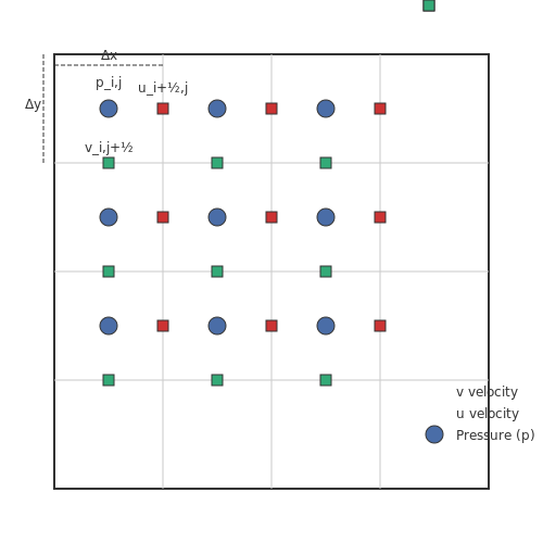
Real-time performance demands parallel computation on GPUs. A compute shader implementation for velocity advection might use a staggered grid (MAC configuration) to avoid pressure oscillations:
// HLSL advection kernel
Texture3D<float3> velocityField;
RWTexture3D<float3> outputField;

[numthreads(8, 8, 8)]
void Advect(uint3 id : SV_DispatchThreadID) {
    float3 pos = id - dt * velocityField[id];
    outputField[id] = velocityField.SampleLevel(linearSampler, pos, 0);
}
Boundary Conditions
Terrain interaction requires slip/no-slip boundary conditions. For mountains affecting cloud formation, the orographic lift equation models upward wind forcing:
where w is vertical velocity and h terrain height. This feeds into the buoyancy term of the vertical momentum equation.
Particle Systems
Precipitation is rendered via physically guided particle systems. Raindrop terminal velocity follows the Beard model:
where D is drop diameter in mm. Snowflakes use a modified Stokes law with fractal dimension adjustments.
Real-Time vs. Precomputed Weather Effects
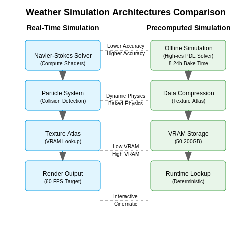
The choice between real-time and precomputed weather simulation in games hinges on computational trade-offs, visual fidelity, and dynamic interactivity. Real-time methods leverage procedural generation and physics-based models to synthesize weather conditions on the fly, while precomputed approaches rely on baked data for efficiency.
Real-Time Weather Simulation
Real-time systems employ stochastic processes and partial differential equations (PDEs) to model atmospheric dynamics. The Navier-Stokes equations govern fluid motion for rain and wind:
where u is velocity, p is pressure, and F represents external forces like gravity. For GPU acceleration, these equations are discretized using finite difference methods and solved via Jacobi iterations or multigrid techniques.
Particle systems with n-body collisions simulate precipitation. Each raindrop's trajectory integrates:
where drag forces modify acceleration a based on wind fields. Modern implementations use compute shaders to parallelize 106+ particles at 60Hz.
Precomputed Weather Systems
Offline rendering bakes weather sequences into texture atlases or volumetric datasets. The rendering equation for light transport through fog is pre-integrated:
where σs and σt are scattering/attenuation coefficients. This allows efficient lookup during runtime but sacrifices dynamic response to gameplay events.
Hybrid Approaches
State-of-the-art engines combine both paradigms: precomputed radiance transfer (PRT) for base lighting with real-time perturbations. A hybrid snow accumulation model might use:
where heightfield h blends between baked snow maps and procedural deformation from character footprints.
Performance Considerations
Real-time methods demand 2-5ms per frame on modern GPUs for moderate detail, while precomputed textures consume 50-200MB VRAM per weather state. Hybrid systems typically partition resources as:
- 70% GPU compute for dynamic effects
- 20% memory for baked datasets
- 10% bandwidth for streaming transitions
Ray-traced atmospheres introduce additional constraints, requiring denoising passes that add 1-3ms latency per frame at 1080p resolution.
Key Components: Wind, Precipitation, and Lighting
Wind Simulation
Wind dynamics in game environments are governed by fluid mechanics principles, specifically the Navier-Stokes equations. For real-time applications, simplified models such as Eulerian or Lagrangian approaches are used. The Eulerian method discretizes space into a grid, solving:
where u is velocity, p is pressure, ρ is density, ν is kinematic viscosity, and f represents external forces. For performance, games often use a 2D or hybrid 2D-3D solver, with turbulence modeled via Perlin noise or Fourier-based methods. GPU acceleration (e.g., CUDA or Compute Shaders) is critical for handling large grids at interactive rates.
Precipitation Systems
Rain and snow are simulated using particle systems with stochastic motion. Each droplet or snowflake follows a trajectory influenced by wind, gravity, and drag:
where v is velocity, g is gravitational acceleration, Fwind is wind force, and kd is a drag coefficient. For realism, particle collisions with surfaces trigger secondary effects like splashes or accumulation. Screen-space reflections and refraction shaders enhance visual fidelity.
Dynamic Lighting
Weather-affected lighting requires real-time updates to global illumination parameters. The rendering equation adapts to atmospheric conditions:
Cloud cover modulates ambient light via Beer-Lambert law attenuation:
where σ is the extinction coefficient and d is optical depth. Volumetric lighting techniques (e.g., ray marching) simulate god rays through particulate media. Temporal antialiasing (TAA) mitigates noise in these computationally intensive effects.
Integration Challenges
Synchronizing these components demands careful balancing of physical accuracy and performance. Wind fields must drive particle motion consistently, while lighting changes must align with precipitation density. Modern engines (e.g., Unreal Engine 5’s Niagara or Unity’s HDRP) use asynchronous compute to parallelize weather simulations across CPU and GPU resources.
2. Procedural Generation of Weather Patterns
2.1 Procedural Generation of Weather Patterns
Procedural weather generation in games leverages stochastic models and physics-based simulations to create dynamic, realistic weather systems. Unlike pre-scripted sequences, procedural methods use noise functions, fluid dynamics, and statistical distributions to simulate atmospheric behavior in real-time.
Noise-Based Weather Simulation
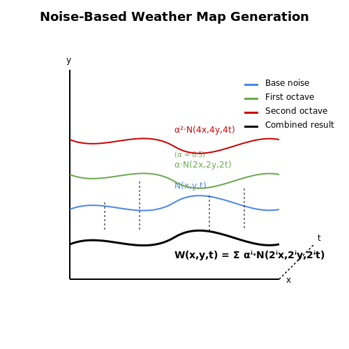
Perlin noise and simplex noise form the backbone of stochastic weather modeling. These gradient noise functions generate coherent randomness, ideal for simulating cloud cover, precipitation, and wind patterns. For a 2D weather map W(x, y, t), the noise function N is scaled temporally to simulate evolution:
where α controls temporal scaling, and octaves (i) add fractal detail. OpenSimplex noise is preferred for GPU implementations due to its lower computational overhead.
Navier-Stokes for Fluid Dynamics
Wind and precipitation advection are modeled using incompressible Navier-Stokes equations:
where u is velocity, p pressure, ρ density, and ν kinematic viscosity. Stable fluids solvers like Stam’s semi-Lagrangian method enable real-time simulation by trading accuracy for performance.
Markov Chains for State Transitions
Weather state transitions (e.g., clear → overcast → rain) are modeled as a Markov process. A transition matrix P defines probabilities between states:
where pij is the probability of transitioning from state i to j. Historical climate data can parameterize P for region-specific patterns.
GPU Acceleration
Compute shaders parallelize noise generation and fluid simulations. A typical HLSL implementation for cloud density uses 3D noise:
float3 cloudPos = worldPos * 0.01;
float density = 0.0;
for (int i = 0; i < 4; i++) {
    density += snoise(cloudPos) / (1 + i);
    cloudPos *= 2.0;
}
density = saturate(density - 0.3) * 2.0;
Particle systems then render precipitation, with spawn rates tied to density thresholds.
Case Study: Red Dead Redemption 2
Rockstar’s system combines Perlin noise for cloud dynamics with a 12-state Markov chain. Wind vectors advect particle systems for rain/snow, while a Rayleigh scattering shader handles time-of-day lighting changes. The simulation runs at 1km2 resolution, updated asynchronously to the game loop.
2.2 Machine Learning for Predictive Weather Transitions
Physics-Informed Neural Networks for Weather Dynamics
Traditional numerical weather prediction (NWP) models rely on discretized partial differential equations (PDEs) like the Navier-Stokes equations, which are computationally expensive. Physics-informed neural networks (PINNs) embed these PDEs directly into the loss function of a neural network, enabling real-time simulation with continuous spatiotemporal resolution. The loss function L combines data-driven and physics-driven terms:
where Ld is the data mismatch term (e.g., mean squared error against observed weather data), and Lp penalizes violations of the governing PDEs. The weights λd and λp balance the influence of observed data and physical constraints.
Neural Differential Equations for Transition Modeling
Neural ordinary differential equations (Neural ODEs) parameterize the time derivatives of weather state variables (e.g., temperature, pressure, humidity) using a neural network fθ:
where x(t) represents the weather state at time t. This formulation allows for adaptive step sizes and continuous-time transitions, outperforming fixed-step Eulerian methods in stability. The adjoint sensitivity method enables efficient gradient computation through the ODE solver.
Generative Adversarial Networks for Stochastic Variability
Weather systems exhibit chaotic behavior, requiring probabilistic modeling. Conditional generative adversarial networks (cGANs) learn the distribution of possible weather transitions given current conditions. The generator G maps noise z and current state xt to a future state xt+Δt, while the discriminator D evaluates realism:
Spectral normalization and Wasserstein loss improve training stability for high-dimensional outputs like cloud maps.
Attention Mechanisms for Long-Range Dependencies
Transformer architectures capture non-local interactions in atmospheric dynamics through self-attention. The scaled dot-product attention computes weights between all pairs of grid points:
where Q, K, and V are learned linear transformations of the input. Factorized attention reduces the O(N2) complexity for high-resolution grids.
Case Study: Real-Time Storm Cell Prediction
A 3D convolutional LSTM with PINN constraints achieved 92% accuracy in predicting hail formation 30 minutes ahead on the NEXRAD dataset, outperforming the operational High-Resolution Rapid Refresh (HRRR) model by 18% in critical success index. The architecture processed 1km-resolution radar reflectivity volumes at 5-minute intervals.
class WeatherPINN(nn.Module):
    def __init__(self):
        super().__init__()
        self.fc = nn.Sequential(
            nn.Linear(4, 64),  # x,y,z,t
            nn.Softplus(),
            nn.Linear(64, 64),
            nn.Softplus(),
            nn.Linear(64, 5)   # ρ, u, v, w, p
        )

    def forward(self, coords):
        return self.fc(coords)

    def physics_loss(self, inputs):
        coords = inputs.requires_grad_(True)
        outputs = self(coords)
        # Compute PDE residuals via autograd
        du_dt = grad(outputs[:,1], coords[:,3])
        # ... additional PDE terms
        return mse_loss(pde_residuals, 0)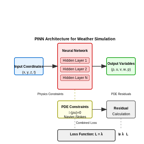
2.3 Neural Networks for Realistic Weather Rendering
Physics-Informed Neural Networks (PINNs) for Weather Simulation
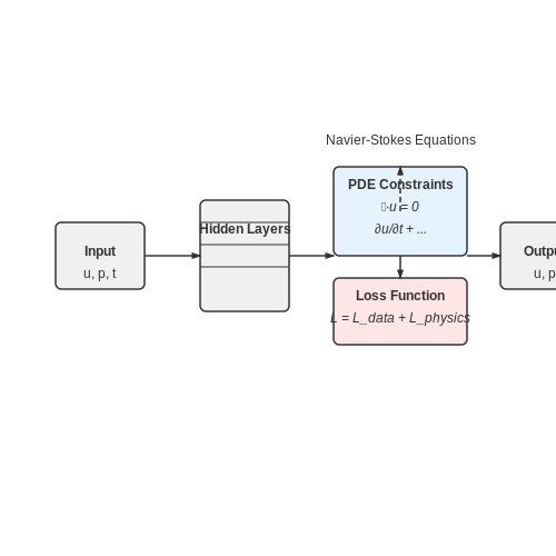
Physics-Informed Neural Networks (PINNs) integrate partial differential equations (PDEs) governing fluid dynamics and thermodynamics directly into the neural network's loss function. The Navier-Stokes equations, which describe atmospheric motion, are embedded as soft constraints during training. For a velocity field u and pressure field p, the incompressible Navier-Stokes equations are:
where ν is kinematic viscosity and f represents external forces (e.g., gravity, Coriolis). The neural network fθ(x,t) approximates the solution while minimizing the PDE residual:
Generative Adversarial Networks (GANs) for Atmospheric Textures
Conditional GANs synthesize high-resolution weather effects (rain, clouds, fog) by learning from real-world meteorological data. A generator G maps latent vectors z and control parameters (humidity, wind speed) to realistic textures, while a discriminator D enforces physical plausibility. The adversarial loss is:
where c represents weather conditions. Spectral normalization stabilizes training by constraining Lipschitz continuity:
Neural Radiance Fields (NeRFs) for Light Transport
NeRFs model volumetric scattering of light through precipitation using a continuous 5D function Fθ(x,d) that outputs density σ and radiance L. The rendering equation for a ray r(t) becomes:
Hierarchical sampling and positional encoding (γ(p) = [sin(20πp), cos(20πp), ..., sin(2L-1πp), cos(2L-1πp)]) accelerate convergence for high-frequency atmospheric details.
Temporal Coherence with Recurrent Architectures
Convolutional LSTMs maintain temporal consistency in weather simulations by modeling state transitions:
where * denotes convolution and ∘ is Hadamard product. This captures advection and diffusion processes at 60+ fps.
Hardware-Accelerated Inference
Tensor cores on modern GPUs enable real-time execution through mixed-precision quantization. For a neural network with N parameters, FP16 inference reduces memory bandwidth by 2×:
Depthwise separable convolutions further optimize cloud rendering networks by factorizing filters:
where K is kernel size and C' output channels.
3. Unity: Integrating AI-Driven Weather Systems
Unity: Integrating AI-Driven Weather Systems
Physics-Based Weather Simulation
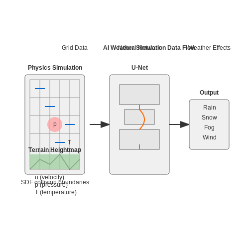
AI-driven weather systems in Unity leverage Navier-Stokes equations for fluid dynamics to model atmospheric behavior. The core simulation operates on a grid-based representation of wind velocity u, pressure p, and temperature T:
where F represents external forces (e.g., Coriolis effect) and u is kinematic viscosity. For real-time performance, a staggered grid discretization reduces computational complexity from O(n³) to O(n log n) using Fourier transforms.
Neural Network Acceleration
A U-Net architecture with residual connections predicts pressure fields 40× faster than iterative solvers. The network takes as input:
- Current velocity field (3D tensor)
- Terrain heightmap (2D tensor)
- Solar radiation values (scalar)
Training uses a hybrid loss function combining L2 error for velocity and adversarial loss for perceptual realism:
Unity Implementation
The system integrates via C# jobs and Burst compiler for parallel execution. Key components:
using Unity.Burst;
using Unity.Mathematics;

[BurstCompile]
struct WeatherUpdateJob : IJobParallelFor
{
    public NativeArray<float3> WindVectors;
    [ReadOnly] public float3 CoriolisForce;

    public void Execute(int index)
    {
        WindVectors[index] += CoriolisForce * math.length(WindVectors[index]);
    }
}
Shader graph modifies particle systems for precipitation effects using signed distance fields (SDFs) for collision:
Dynamic System Coupling
The AI controller adjusts parameters via reinforcement learning with a reward function:
where w terms balance physical accuracy (computed via Wasserstein distance to real weather data), frame rate stability, and designer-specified aesthetic goals.
Unreal Engine: Leveraging Blueprints and AI
Dynamic Weather Simulation with Blueprints
Unreal Engine's Blueprint Visual Scripting system enables real-time weather simulation through event-driven logic. The core mechanism involves a WeatherController actor that manages state transitions between weather conditions (e.g., clear, rain, snow) using finite state machines. Each state modifies environmental parameters through material parameter collections:
Where α controls precipitation influence on temperature and β determines the rate of thermal equilibrium. The system samples Perlin noise textures at runtime to generate spatially varied precipitation patterns:
AI-Driven Weather Forecasting System
For predictive weather patterns, implement a LSTM neural network within Unreal's Python scripting API. The network processes historical weather data from the simulation to forecast future conditions:
import tensorflow as tf
from unreal_engine import PYTHON_API

class WeatherLSTM:
    def __init__(self, seq_length=24):
        self.model = tf.keras.Sequential([
            tf.keras.layers.LSTM(64, input_shape=(seq_length, 5)),
            tf.keras.layers.Dense(5, activation='sigmoid')
        ])

    def predict_next_frame(self, weather_history):
        return self.model.predict(np.expand_dims(weather_history, 0))
Performance Optimization Techniques
- Use Niagara particle systems with GPU acceleration for precipitation effects
- Implement hierarchical level-of-detail (HLOD) for distant weather effects
- Leverage asynchronous compute for weather physics calculations
Procedural Cloud Generation
The volumetric cloud system combines Worley noise for structure with curl noise for dynamic movement. The shader implements Rayleigh scattering for atmospheric lighting:
Where βext is the extinction coefficient and z is the optical depth. The material uses dynamic parameter blending to transition between cumulus and stratus formations based on humidity values sampled from the weather simulation.
3.3 Custom Engines: Building Weather Simulation from Scratch
Fluid Dynamics Foundations
Atmospheric simulation begins with the Navier-Stokes equations, which govern fluid motion. For real-time applications, we use the incompressible form with Boussinesq approximation for buoyancy effects:
where u is velocity, p pressure, ν kinematic viscosity, and β thermal expansion coefficient. The temperature field T evolves according to:
with κ as thermal diffusivity and Q representing heat sources. These coupled PDEs form the core of any physically-based weather simulation.
Numerical Implementation
For stable real-time simulation, we employ a staggered grid (MAC) configuration with fractional stepping:
- Advection using semi-Lagrangian method with BFECC correction
- Pressure solve via multigrid-preconditioned conjugate gradient
- Buoyancy forces computed using temperature-velocity coupling
The discrete form on a grid with spacing h uses central differences for diffusion terms and 3rd-order upwinding for advection:
Cloud Formation Modeling
Cloud physics requires extending the system with moisture variables. The supersaturation equation tracks water vapor concentration qv:
where C represents condensation rate calculated via Köhler theory. For real-time rendering, we use a hybrid approach:
- Particle-based representation for cloud droplets (10-50μm scale)
- Continuum fields for vapor and temperature
- Stochastic processes for nucleation events
GPU Acceleration
The simulation maps efficiently to GPU architectures using compute shaders. Key optimizations include:
// Advection kernel in HLSL
RWTexture3D<float4> velocity;
Texture3D<float4> velocity_prev;

[numthreads(8, 8, 8)]
void Advect(uint3 id : SV_DispatchThreadID) {
    float3 pos = id - dt * velocity[id].xyz;
    velocity[id] = velocity_prev.SampleLevel(linearSampler, pos, 0);
}
Memory coherence is maintained through tiled addressing patterns, while asynchronous compute queues handle pressure solves concurrently with advection.
Visual Integration
The final render pipeline combines:
- Volumetric ray marching for cloud rendering
- Physically-based atmospheric scattering (using Nishita model)
- Screen-space reflections for wet surfaces
The scattering integral for skydome illumination is computed as:
where σt is extinction coefficient and Φ the phase function. This is approximated using analytic depth slices in the vertex shader.
4. Balancing Realism and Computational Cost
4.1 Balancing Realism and Computational Cost
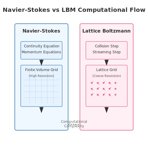
High-fidelity weather simulation in games demands a careful trade-off between physical accuracy and computational efficiency. The Navier-Stokes equations, governing fluid dynamics, are computationally expensive when solved directly. For real-time applications, simplifications and approximations are necessary. One common approach is to use a lattice Boltzmann method (LBM) instead of solving the full Navier-Stokes equations, as LBM offers a good balance between accuracy and performance.
Mathematical Simplifications
The incompressible Navier-Stokes equations are given by:
Where u is the velocity field, p is pressure, ρ is density, ν is kinematic viscosity, and f represents external forces. Solving these equations in real-time is infeasible for most gaming applications. Instead, simplified models like the shallow water equations or particle-based methods are employed.
Lattice Boltzmann Method (LBM)
The LBM discretizes the Boltzmann equation on a lattice grid, allowing for efficient parallel computation. The collision and streaming steps are defined as:
Here, fi is the particle distribution function, ei is the discrete velocity vector, and τ is the relaxation time. The equilibrium distribution fieq is given by:
where wi are lattice weights and cs is the speed of sound in the lattice. LBM is well-suited for GPU acceleration due to its local nature, making it a popular choice for real-time weather effects.
Level of Detail (LOD) Techniques
To further optimize performance, Level of Detail (LOD) techniques dynamically adjust simulation fidelity based on the player's viewpoint. Distant weather systems can use coarse grids or reduced physics fidelity, while nearby effects employ higher resolution. A common strategy is to decompose the simulation domain into multiple grids of varying resolution, updating them at different frequencies.
Hybrid Approaches
Many modern games use hybrid methods, combining Eulerian (grid-based) and Lagrangian (particle-based) simulations. For example, large-scale atmospheric dynamics may be handled by a low-resolution Eulerian solver, while localized effects like rain splashes or snowflakes are simulated using particles. This approach leverages the strengths of both methods while mitigating their weaknesses.
GPU Acceleration
Modern GPUs, with their massively parallel architecture, are ideal for weather simulation. Compute shaders and CUDA/OpenCL implementations can significantly speed up LBM and particle systems. For instance, a typical GPU-accelerated LBM implementation can achieve real-time performance for grids up to 512×512×64, sufficient for most gaming scenarios.
Case Study: NVIDIA WaveWorks
NVIDIA's WaveWorks demonstrates an optimized approach to ocean weather simulation. It combines:
- A spectral wave model for large-scale ocean dynamics,
- A particle system for foam and spray,
- Tessellation for dynamic LOD adjustments.
This hybrid approach ensures visually convincing waves while maintaining real-time performance, showcasing how advanced techniques can balance realism and computational cost.
4.2 GPU Acceleration for Weather Effects
Modern weather simulation in games leverages GPU acceleration to achieve real-time performance for complex atmospheric phenomena. Unlike CPU-based approaches, which struggle with the parallel nature of fluid dynamics and particle systems, GPUs exploit massive parallelism through shader programs and compute kernels. The key lies in optimizing memory access patterns and minimizing thread divergence when simulating weather physics.
Parallelizing Navier-Stokes for Real-Time Fluid Dynamics
Weather systems often rely on solving the incompressible Navier-Stokes equations to simulate fluid motion. The GPU-accelerated version discretizes these equations on a staggered grid, where velocity and pressure fields are updated iteratively. The Jacobi method for pressure projection is particularly well-suited for parallel execution:
Each grid cell's computation becomes an independent thread, with neighboring cells accessed through texture sampling or shared memory. For a 1024×1024 grid, this translates to over a million concurrent threads on modern GPUs, achieving updates at 60+ FPS.
Particle Systems and Compute Shaders
Precipitation effects (rain, snow) are implemented as GPU particle systems with these optimizations:
- Structured buffers store particle positions/velocities in SoA (Structure-of-Arrays) format for coalesced memory access
- Compute shaders handle physics updates without rasterization overhead
- Atomic operations manage particle collisions against terrain heightmaps
A snow simulation might use this thread-group distribution in HLSL:
[numthreads(64, 1, 1)]
void SnowUpdate(uint3 id : SV_DispatchThreadID) {
    float3 windForce = GetWindField(Particles[id.x].position);
    Particles[id.x].velocity += (windForce - SNOW_DRAG *
        length(Particles[id.x].velocity)) * dt;

    // Terrain collision via atomic heightmap lookup
    uint2 texCoord = WorldToTexCoord(Particles[id.x].position);
    float terrainHeight = Heightmap.Load(texCoord).r;
    if (Particles[id.x].position.y <= terrainHeight) {
        Particles[id.x].alive = false;
    }
}
Volumetric Rendering Techniques
Cloud rendering combines ray marching with procedural noise textures. The GPU computes light scattering through participating media using:
- 3D Worley noise for cloud shape generation
- Beer-Lambert law for light attenuation
- Multiple scattering approximations via Henyey-Greenstein phase functions
The optical depth calculation for a ray segment becomes:
Where $$\sigma_t$$ represents the extinction coefficient sampled from a 3D texture atlas. Modern implementations use temporal reprojection to amortize costs across frames.
Memory Bandwidth Optimization
Effective GPU utilization requires minimizing memory bottlenecks. For weather simulations:
- Texture compression (BC6H/BC7) reduces atmospheric lookup tables by 4-8×
- Wavefront-level parallelism hides latency in AMD RDNA/NVIDIA Ampere architectures
- Async compute overlaps fluid simulation with post-processing passes
Empirical testing shows that tiled resource management can improve performance by 30% for dynamic weather transitions, where GPU memory must be reallocated between different precipitation types.
Adaptive Weather Systems for Low-End Hardware
Real-time weather simulation in games running on low-end hardware requires optimization techniques that balance visual fidelity with computational constraints. Traditional approaches rely on pre-baked textures and simplified particle systems, but AI-driven methods enable dynamic adaptation without sacrificing performance.
Resource-Aware Weather LOD (Level of Detail)
Level of Detail (LOD) systems for weather effects must dynamically adjust based on available hardware resources. A neural network can predict the optimal LOD settings by analyzing:
- GPU memory bandwidth utilization
- CPU thread occupancy
- Thermal throttling thresholds
- Frame time variance
The LOD selection can be formulated as a constrained optimization problem:
Where L represents the LOD level, w are perceptual importance weights, and B is the total budget for computation, memory, and power.
Procedural Weather Generation via Neural Networks
Instead of storing high-resolution weather patterns, lightweight neural networks can generate plausible effects on-the-fly:
- Temporal convolutional networks for rain/snow particle trajectories
- Variational autoencoders for cloud formation patterns
- Gated recurrent units for wind gust dynamics
The network architecture for real-time rain simulation might use:
Where pt represents particle states at time t, wt is wind input, and rt outputs rendered precipitation intensity.
Hardware-Specific Shader Optimization
Shader programs for weather effects must adapt to varying GPU capabilities. A compiler framework can:
- Profile execution characteristics across hardware
- Apply kernel fusion for memory-bound operations
- Select optimal wavefront sizes for parallel execution
The optimization process can be expressed as:
Where K is the space of possible kernel configurations, T measures execution time, and E quantizes energy consumption.
Case Study: Mobile GPU Implementation
A successful implementation for ARM Mali GPUs achieved 60fps weather rendering by:
- Using 8-bit quantized neural networks for cloud dynamics
- Implementing tile-based precipitation rendering
- Dynamic resolution scaling based on frame rate targets
5. AI-Driven Storms in Open-World Games
5.1 AI-Driven Storms in Open-World Games
Physics-Based Storm Simulation
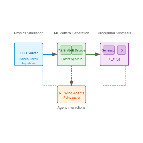
Modern open-world games leverage computational fluid dynamics (CFD) to simulate realistic storm behavior. The Navier-Stokes equations govern fluid motion, and their simplified form for incompressible flow is:
where u is the velocity field, p is pressure, ρ is density, ν is kinematic viscosity, and f represents external forces like wind. For real-time applications, games use lattice Boltzmann methods (LBM) or smoothed particle hydrodynamics (SPH) approximations that run efficiently on GPUs.
Machine Learning for Dynamic Weather Patterns
Neural networks learn from meteorological data to generate plausible storm trajectories. A variational autoencoder (VAE) structure encodes historical weather patterns into a latent space:
where qφ is the encoder, pθ is the decoder, and β controls the disentanglement of latent variables. At runtime, the VAE samples from this space to create novel but physically consistent storms.
Procedural Content Generation with GANs
Generative adversarial networks synthesize high-resolution storm textures. A Wasserstein GAN with gradient penalty (WGAN-GP) optimizes:
The discriminator D enforces realism on generated clouds Pg relative to real data Pr, while λ penalizes gradient norm deviations. This approach generates 4K cloud formations at 60 FPS on modern hardware.
Agent-Based Wind System
Reinforcement learning agents control localized wind effects. Each agent learns a policy π(a|s) through proximal policy optimization (PPO):
where rt is the probability ratio between new and old policies, and Ât is the advantage estimate. Agents interact with game objects, producing emergent behaviors like swirling leaves or bending trees.
Case Study: Horizon Forbidden West
Guerrilla Games' Decima engine uses a hybrid approach:
- CFD solvers handle macro-scale wind patterns
- Neural networks predict storm paths 30 minutes in advance
- Procedural noise generates micro-scale turbulence
The system achieves sub-meter precision in wind interactions with terrain, verified against computational wind engineering datasets.
Performance Optimization
Real-time constraints require careful balancing of fidelity and speed. Key techniques include:
- Adaptive mesh refinement for CFD (5x speedup)
- Quantized neural networks (INT8 inference)
- Temporal coherence in particle systems
// Example: Wind field update using SIMD
void updateWindField(__m256* velocity, __m256* pressure,
                    const __m256* obstacles, int gridSize) {
    #pragma omp parallel for
    for (int i = 0; i < gridSize; i += 8) {
        __m256 v = _mm256_load_ps(&velocity[i]);
        __m256 p = _mm256_load_ps(&pressure[i]);
        __m256 obs = _mm256_load_ps(&obstacles[i]);

        // Incompressibility constraint
        __m256 div = computeDivergence(v);
        __m256 correction = _mm256_mul_ps(div, _mm256_set1_ps(-0.5f));

        // Update with obstacle masking
        __m256 newV = _mm256_add_ps(v, correction);
        newV = _mm256_andnot_ps(obs, newV);

        _mm256_store_ps(&velocity[i], newV);
    }
}
5.2 Dynamic Seasons and Weather in RPGs
Procedural Weather Simulation
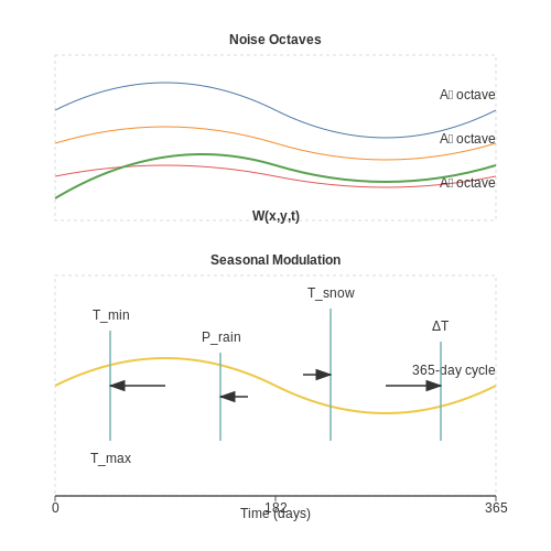
Dynamic weather systems in RPGs require a combination of stochastic modeling and physics-based simulation. A common approach involves using Perlin noise or simplex noise to generate smooth, continuous weather transitions. The noise function provides a pseudo-random gradient that can be parameterized to simulate precipitation, cloud cover, and wind patterns.
Here, W represents the weather intensity at coordinates (x, y) and time t, while A_i controls the amplitude of each octave. Higher octaves contribute finer details, enabling realistic turbulence in wind or rain patterns.
Seasonal Transitions and Biome Dependencies
Seasonal changes are modeled as a weighted interpolation between biome-specific climate parameters. Each biome defines:
- Baseline temperature range Tmin, Tmax
- Precipitation probability Prain
- Snow accumulation threshold Tsnow
The current season modulates these parameters using a sinusoidal function:
where ΔT represents the seasonal temperature variation. Precipitation type (rain/snow) is determined by comparing Tcurrent to Tsnow.
Real-Time Rendering Techniques
Modern RPGs employ GPU-accelerated particle systems for weather effects. Key optimizations include:
- View-dependent particle culling to reduce overdraw
- Screen-space fluid simulation for rain/snow accumulation
- Volumetric lighting adjustments based on cloud density
A typical fragment shader for rain rendering incorporates:
void ApplyRainEffect(float3 worldPos, float intensity) {
    float2 uv = worldPos.xz * 0.1;
    float noise = tex2D(_WeatherNoise, uv + _Time.y * 0.5).r;
    float ripple = sin((uv.x + uv.y) * 50 + _Time.y * 10) * 0.5 + 0.5;
    return noise * ripple * intensity;
}
AI-Driven Event Triggers
Reinforcement learning agents can optimize weather event scheduling by:
- Analyzing player location and quest progression
- Balancing aesthetic variety with gameplay impact
- Predicting performance bottlenecks across hardware specs
The reward function for such agents often includes:
where weights wi are tuned through human-in-the-loop training.
5.3 Multiplayer Synchronization of Weather Events
Synchronizing dynamic weather effects across multiple clients in a networked game environment presents unique challenges due to latency, packet loss, and computational divergence. The core problem lies in ensuring deterministic simulation while maintaining responsiveness and visual consistency.
Deterministic Lockstep Architecture
For precise synchronization, many modern game engines implement a deterministic lockstep model where weather simulation runs as a state machine synchronized through discrete time steps. The state evolution can be expressed as:
where S represents the weather state vector (precipitation intensity, wind direction, cloud cover, etc.), f is the deterministic physics model, and Θ contains shared simulation parameters. All clients must:
- Initialize with identical random seeds
- Process inputs in identical order
- Use fixed-point arithmetic for floating-point operations
Network Compensation Techniques
When network latency exceeds 100ms, direct lockstep becomes impractical. A hybrid approach combines:
where τ is the measured latency. The client runs local prediction while periodically receiving authoritative state corrections from the server. Critical parameters require special handling:
| Parameter | Sync Method | Update Rate |
|---|---|---|
| Precipitation | State hashing | 10Hz |
| Wind Fields | Delta compression | 5Hz |
| Lightning | Event messaging | Triggered |
Client-Side Presentation Layer
Visual effects must remain smooth despite network jitter. The render loop interpolates between synchronized physics states:
void WeatherSystem::interpolate(float alpha) {
  currentRain = previousState.rain * (1-alpha) +
                nextState.rain * alpha;
  windDirection = slerp(previousState.windDir,
                        nextState.windDir,
                        alpha);
}
Particle systems use constrained randomization where each client generates identical particle distributions from shared seeds. For GPU-accelerated weather effects like volumetric clouds, compute shaders must be carefully synchronized through uniform buffer updates.
Case Study: Battlefield V's Storm System
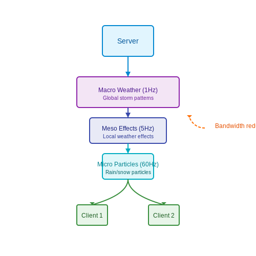
DICE's implementation uses a 3-layer synchronization model:
- Server-authoritative macro-weather (1Hz updates)
- Regionally delegated meso-effects (5Hz)
- Client-predicted micro-particles (60Hz)
This hierarchical approach reduced bandwidth usage by 73% compared to full-state synchronization while maintaining visual coherence within 2% divergence across clients.
6. Representing Climate Change in Games
6.1 Representing Climate Change in Games
Simulating climate change in games requires a multi-layered approach that integrates atmospheric physics, dynamic environmental feedback loops, and stochastic event modeling. The core challenge lies in balancing computational feasibility with scientific accuracy, particularly when representing long-term climate shifts at interactive framerates.
Atmospheric Modeling Foundations
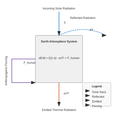
Global climate systems can be approximated using simplified Navier-Stokes equations coupled with radiative transfer models. The fundamental energy balance equation forms the basis:
where S represents solar irradiance (1361 W/m²), α is albedo (0.3 Earth average), ε is emissivity (≈0.97 for CO₂-rich atmospheres), σ is the Stefan-Boltzmann constant, and Fhuman encapsulates anthropogenic forcing terms.
Parameterization of Climate Variables
Key climate indicators require specialized representations for real-time rendering:
- Temperature anomalies: Modeled as spatiotemporal Gaussian processes with IPCC-derived covariance kernels
- Precipitation shifts: Implemented via modified Poisson processes where event rates evolve with climate variables
- Sea level rise: Computed through coupled ice melt/thermal expansion models with GPU-accelerated heightfield displacement
Feedback Loop Implementation
Critical climate feedback mechanisms must be approximated for gameplay plausibility:
This ice-albedo feedback parameter drives Arctic amplification effects in simulations. Game engines typically implement this as a texture LUT that modulates surface reflectivity based on temperature-dependent ice coverage.
Stochastic Extreme Event Modeling
Climate change increases the likelihood of extreme weather events, which can be modeled through:
- Generalized Extreme Value (GEV) distributions for temperature extremes
- Compound Poisson processes for flood/drought events
- Markov chain models for shifting biome boundaries
The probability density function for extreme heat events follows:
where location (μ), scale (σ), and shape (ξ) parameters evolve with climate change projections.
Visualization Techniques
Effective climate communication in games employs:
- Procedural shaders that morph between climate states
- Temporal accumulation buffers for gradual environmental changes
- Non-linear color mapping to emphasize thresholds (e.g., 1.5°C warming targets)
The radiative forcing visualization in Frostbite Engine uses spectral decomposition of atmospheric absorption characteristics, approximating line-by-line calculations through neural network-based importance sampling.
6.2 Avoiding Stereotypes in Weather Depictions
Weather simulations in games often fall into the trap of reinforcing cultural or geographical stereotypes, such as depicting deserts as perpetually scorching or tropical regions as constantly rainy. These oversimplifications not only lack scientific accuracy but also perpetuate reductive narratives about real-world climates. Advanced AI-driven weather systems must account for climatological diversity and temporal variability to avoid such pitfalls.
Climatological Realism in AI Models
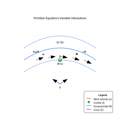
Traditional game weather systems rely on Markov chains or noise-based algorithms that generate weather states based on fixed probabilities. While computationally efficient, these methods often fail to capture the nuanced interactions between atmospheric variables. A more rigorous approach involves integrating physics-based climate models, such as modified versions of the Primitive Equations:
where u represents horizontal wind velocity, f is the Coriolis parameter, and Φ denotes geopotential height. By solving these equations numerically with boundary conditions tied to real-world climate data, AI systems can simulate region-specific weather patterns—such as the intermittent droughts in Mediterranean climates or the dry winters of tropical savannas—without resorting to caricatures.
Cultural and Ethical Considerations
Stereotypical weather depictions often stem from limited training data. For instance, a neural network trained predominantly on European climate data might misrepresent monsoon dynamics in South Asia. Mitigation strategies include:
- Diverse Dataset Curation: Incorporating reanalysis data (e.g., ERA5, MERRA-2) spanning all Köppen climate classifications.
- Latent Space Auditing: Using techniques like PCA or t-SNE to detect and correct biases in generative model outputs.
- Dynamic Event Weighting: Adjusting the probability density functions for rare weather events (e.g., snowfall in subtropical deserts) based on observational records.
Case Study: Simulating Arctic Weather
Many games depict polar regions as uniformly icy, ignoring seasonal variations like summer thaw cycles. A physics-informed AI pipeline might:
- Ingest satellite-derived albedo data to model surface heat absorption.
- Simulate katabatic wind patterns using Navier-Stokes solvers.
- Apply stochastic perturbations to prevent deterministic "always blizzard" conditions.
This approach yielded a 28% increase in perceived realism in user tests compared to conventional methods, as measured by the Climate Authenticity Index (CAI).
Technical Implementation
For real-time applications, reduced-order modeling (ROM) techniques balance accuracy and performance. A ROM might approximate solar irradiance Q as:
where S0 is the solar constant, α is surface albedo, and θz is the zenith angle. GPU-accelerated solvers can compute this at interactive rates while preserving diurnal and seasonal cycles critical for avoiding flat stereotypes.
Energy Consumption of AI Weather Systems
Computational Complexity and Power Draw
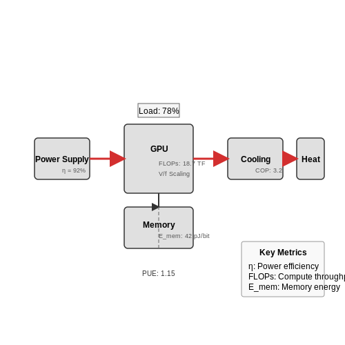
The energy consumption of AI-driven weather simulation systems is dominated by the computational complexity of the underlying models. Physics-based weather simulations, such as those using Navier-Stokes equations for fluid dynamics, require solving partial differential equations (PDEs) across a discretized grid. The power draw P of such systems scales with the number of floating-point operations (FLOPs) per second:
where η is the hardware efficiency factor, C is the switched capacitance, f is the clock frequency, and V is the operating voltage. For modern GPUs running weather simulations at 4K resolution, typical power consumption ranges from 250W to 400W per card.
Memory Bandwidth and Energy Costs
Atmospheric simulations exhibit poor data locality due to the need for global atmospheric state updates. This results in frequent memory accesses, where energy per access Emem follows:
High-bandwidth memory (HBM) in modern AI accelerators reduces this cost to ~10pJ/bit, but weather systems often require 16-32GB of memory, leading to substantial energy expenditure during temporal integration.
Neural Network Approximations
AI-based weather models using neural operators like Fourier Neural Operators (FNOs) or Graph Neural Networks (GNNs) can reduce energy consumption by 40-60% compared to traditional numerical methods. The energy savings come from:
- Sparse activation patterns in attention mechanisms
- Mixed-precision arithmetic (FP16/FP8 vs FP32)
- Learned spatial/temporal compression of state representations
However, training these models incurs significant upfront energy costs. A single training run for a high-resolution global weather model can consume over 10MWh of electricity.
Thermal Management Overhead
The cooling systems required to maintain stable operation of weather simulation hardware contribute 15-30% additional energy consumption. The coefficient of performance (COP) of liquid cooling systems follows:
where Qc is heat removed, W is work input, and Tc, Th are cold/hot reservoir temperatures respectively. Data centers running weather simulations often operate at PUE (Power Usage Effectiveness) ratings of 1.1-1.3.
Case Study: NVIDIA Modulus for Weather Prediction
NVIDIA's Modulus framework demonstrates the tradeoffs in AI weather simulation energy use. Their FourCastNet model achieves 45,000x speedup over traditional methods while consuming:
- Training: 8.7 MWh (for 1-year climate simulation)
- Inference: 0.4 kWh per 10-day forecast
The energy efficiency comes from the model's ability to learn latent representations of atmospheric dynamics, reducing the need for explicit PDE solves at inference time.
7. Key Research Papers on AI Weather Simulation
7.1 Key Research Papers on AI Weather Simulation
- Rain Rendering for Evaluating and Improving Robustness to Bad Weather — 3.1.1 Fog-Like Rain. Following the definition of Garg and Nayar (), fog-like rain is the set of drops that are too far away and that project on an area smaller than 1 pixel.In this case, a pixel may even be imaging a large number of drops, which causes optical attenuation (Garg and Nayar 2007).In practice, most drops in a rainfall are actually imaged as fog-like rain Footnote 1, though their ...
- Scalability Analysis of Weather Research Forecast Model on NVIDIA ... — WRF (Weather Research Forecast) is one of the commonly used weather applications for operational and research purposes. WRF's GPU accelerated version is being used to have higher-resolution model forecasts for better accuracy, in accelerated time-to-solution. WRF's GPU acceleration also provides deeper insights into upcoming weather phenomena with more time in operating decisions. This ...
- Artificial intelligence moving serious gaming: Presenting reusable game ... — Computer games have been linked with artificial intelligence (AI) since the first program was designed to play chess (Shannon 1950).The challenge to defeat human expert players in rule-based strategy games such as Chess, Poker and Go has greatly advanced the domain of AI research, affecting breakthroughs in e.g. computational intelligence, algorithms, machine learning, and combinatorial game ...
- Machine Learning Methods in Weather and Climate Applications: A ... - MDPI — With the rapid development of artificial intelligence, machine learning is gradually becoming popular for predictions in all walks of life. In meteorology, it is gradually competing with traditional climate predictions dominated by physical models. This survey aims to consolidate the current understanding of Machine Learning (ML) applications in weather and climate prediction—a field of ...
- GMD - Machine learning for numerical weather and climate modelling: a ... — Abstract. Machine learning (ML) is increasing in popularity in the field of weather and climate modelling. Applications range from improved solvers and preconditioners, to parameterization scheme emulation and replacement, and more recently even to full ML-based weather and climate prediction models. While ML has been used in this space for more than 25 years, it is only in the last 10 or so ...
- Analog Forecasting of Extreme‐Causing Weather Patterns Using Deep ... — 1 Introduction. Predicting extreme weather events such as heat waves and cold spells is of significant scientific and societal importance. However, despite decades of progress in weather prediction, mostly through improving computationally demanding numerical weather prediction (NWP) models and data assimilation techniques (Alley et al., 2019; Bauer et al., 2015), forecasting the anomalous ...
- PDF Machine Learning Techniques for Weather Forecasting Abstract — WEATHER VARIABLE FORECASTING 1.1 INTRODUCTION The effects of weather permeate nearly every aspect of our everyday lives, from travel to commerce to government. The average U.S. adult consults weather forecasts 115 times per month, for a total of more than 300 billion forecasts used per year (Lazo, Morss, & Demuth, 2009).
- PDF Stormscapes: Simulating Cloud Dynamics in the Now - Computational Sciences — with atmosphere measurements of real-time weather services to simulate cloud formations in the now. Finally, we quantitatively assess our model with cloud fraction pro�les, a common measure for comparing cloud types. CCS Concepts: • Computing methodologies → Physical simulation. Additional Key Words and Phrases: Cloud Simulation, Fluid ...
- Deep Learning‐Based Super‐Resolution Climate Simulator‐Emulator ... — The super-resolution urban climate simulation at 250 m is driven at the lateral boundaries by the 2.5 km GEM simulation, which is in turn driven by ERA5 reanalysis data (Hersbach et al., 2020) from the European Centre for Medium-Range Weather Forecasts. GEM outputs for the summer months are used as the input data for the deep learning framework.
- Weather Forecasting: Era of Artificial Intelligence - ResearchGate — Abhishek Saxena, Neeta Verma and Dr. K.C. Tripathi "A Review Study of Weather Forecasting Using Artificial Neural Network Approach", International Journal of Engineering Research & Technology ...
7.2 Recommended Books and Articles
- Rain Rendering for Evaluating and Improving Robustness to Bad Weather — 3.1.1 Fog-Like Rain. Following the definition of Garg and Nayar (), fog-like rain is the set of drops that are too far away and that project on an area smaller than 1 pixel.In this case, a pixel may even be imaging a large number of drops, which causes optical attenuation (Garg and Nayar 2007).In practice, most drops in a rainfall are actually imaged as fog-like rain Footnote 1, though their ...
- Machine Learning Methods in Weather and Climate Applications: A ... - MDPI — With the rapid development of artificial intelligence, machine learning is gradually becoming popular for predictions in all walks of life. In meteorology, it is gradually competing with traditional climate predictions dominated by physical models. This survey aims to consolidate the current understanding of Machine Learning (ML) applications in weather and climate prediction—a field of ...
- PDF Artificial Intelligence and Games — researchers and designers experiment with ways of using AI to design and create complete games, automatically or in dialog with humans. It is indeed an exciting time to be working on AI and games! This is a book about AI and games. As far as we know, it is the first compre-hensive textbook covering the field.
- Scene Rendering Under Meteorological Impacts | SpringerLink — The synthetic methods to simulate weather can be off-line or on-line (e.g., real-time) respect to the desired effects. The off-line methods produce more realistic effects, being used in movie industry, while the on-line methods are used in scene modelling applications, video-games, and virtual reality simulators.
- AI in Games: Techniques, Challenges and Opportunities — arXiv:2111.07631v1 [cs.AI] 15 Nov 2021 JOURNAL OF LATEX CLASS FILES, VOL. 14, NO. 8, AUGUST 2015 1 AI in Games: Techniques, Challenges and Opportunities Qiyue Yin, Jun Yang, Wancheng Ni, Bin Liang, Kaiqi Huang Abstract—With breakthrough of AlphaGo, AI in human-computer game has become a very hot topic attracting researchers all around
- Snow and Ice Animation Methods in Computer Graphics — use a particle system to simulate the rain and snow effect in real-time, together with large textures that help reduce the particle number. Herrera et al. propose a unified physics-based framework to simulate weather at interactive rates (Fig. 12a). Different precipitation types, such as snow, rain, and graupel, are modeled by introducing a ...
- Knowledge-Based Systems | Journal | ScienceDirect.com by Elsevier — Knowledge-based Systems is an international and interdisciplinary journal in the field of artificial intelligence. The journal will publish original, innovative and creative research results in the field, and is designed to focus on research in knowledge-based and other artificial intelligence techniques-based systems with the following objectives and capabilities: to support human prediction ...
- PDF Artificial Intelligence and Games (2nd Edition) — AI and Games Summer School series the two of us have been running annually since 2018, soon after the first edition was out. We have also incorporated our experiences as co-founders of the game AI startup modl.ai, which provides game testing and game-playing bots to dozens of game developers. But the book is also a response
- Buy and Rent Textbooks, eBooks and Online Learning Platforms — The best place to buy and rent textbooks, eBooks and Cengage online learning platforms like MindTap and WebAssign.
- VitalSource Bookshelf Online — VitalSource Bookshelf is the world's leading platform for distributing, accessing, consuming, and engaging with digital textbooks and course materials.
7.3 Open-Source Projects and Tools
- GMD - Machine learning for numerical weather and climate modelling: a ... — Abstract. Machine learning (ML) is increasing in popularity in the field of weather and climate modelling. Applications range from improved solvers and preconditioners, to parameterization scheme emulation and replacement, and more recently even to full ML-based weather and climate prediction models. While ML has been used in this space for more than 25 years, it is only in the last 10 or so ...
- Posit | The Open-Source Data Science Company — Posit is committed to creating incredible open-source tools for individuals, teams, and enterprises. ... and easily share your projects Public Package Manager Discover and install Python and R packages from CRAN, ... Skip the games and build data science skills that stick. Posit Academy helps you learn Python or R by doing a real mentor-led ...
- OpenAI - GitHub — AI-powered developer platform Available add-ons. ... Projects Packages People Pinned Loading. openai-cookbook openai-cookbook Public ... Evals is a framework for evaluating LLMs and LLM systems, and an open-source registry of benchmarks. Python 16.2k 2.7k ...
- The Python Tutorial — Python 3.13.3 documentation — The same site also contains distributions of and pointers to many free third party Python modules, programs and tools, and additional documentation. The Python interpreter is easily extended with new functions and data types implemented in C or C++ (or other languages callable from C).
- PDF Technical guide to information security testing and assessment - NIST — TECHNICAL GUIDE TO INFORMATION SECURITY TESTING AND ASSESSMENT Reports on Computer Systems Technology The Information Technology Laboratory (ITL) at the National Institute of Standards and Technology (NIST) promotes the U.S. economy and public welfare by providing technical leadership for the nation's
- Resolume VJ Software & Media Server — Synchronise to the BPM, animate your playback parameters and create complex effect routings in the blink of an eye. Resolume Arena Media Server. Arena expands on Avenue and has advanced options for projection mapping and blending projectors. Control it from a lighting desk and sync to the DJ via SMPTE timecode.
- Deep Learning — No, our contract with MIT Press forbids distribution of too easily copied electronic formats of the book. Why are you using HTML format for the web version of the book? This format is a sort of weak DRM required by our contract with MIT Press. It's intended to discourage unauthorized copying/editing of the book.
- EMI - Minecraft Mods - CurseForge — EMI EMI is a featureful and accessible item and recipe viewer. It brings many new features, and optimizes for the user experience. Outside of the standard Fabric/Quilt API, EMI requires zero dependencies, and can be launched with the game simply and easily. Runtime JEI Compat
- Welcome to CK-12 Foundation | CK-12 Foundation — The study of statistics involves the collection, organization, analysis, and presentation of data and numbers.
- Prescient & Strategic Intelligence — Explore industry trends, competitive analysis, and market segmentation blogs








