Reformer: Efficient Transformers with LSH
1. Core Architecture of Transformers
1.1 Core Architecture of Transformers
The transformer architecture, introduced by Vaswani et al. in 2017, revolutionized sequence modeling by replacing recurrent and convolutional layers with self-attention mechanisms. At its core, the transformer consists of an encoder-decoder structure, though many modern variants (e.g., BERT, GPT) use only one of these components. The key innovation lies in the scaled dot-product attention mechanism, which enables direct modeling of relationships between all positions in a sequence.
Self-Attention Mechanism
Given an input sequence of embeddings X ∈ ℝn×d, where n is the sequence length and d is the embedding dimension, the self-attention mechanism projects X into three matrices:
where WQ, WK ∈ ℝd×dk and WV ∈ ℝd×dv are learned projection matrices. The attention weights are computed as:
The scaling factor 1/√dk prevents the dot products from growing too large in magnitude, which would push the softmax into regions with extremely small gradients.
Multi-Head Attention
Transformers employ h parallel attention heads to jointly attend to information from different representation subspaces:
where each head computes attention independently with different learned projections:
The output projection WO ∈ ℝhdv×d combines the results from all heads. This architecture allows the model to capture diverse relationships at different positions and representation subspaces.
Position-wise Feed-Forward Networks
Each transformer layer contains a fully connected feed-forward network (FFN) applied independently to each position:
where W1 ∈ ℝd×dff, W2 ∈ ℝdff×d, and dff is typically 4×d. This provides additional nonlinear transformations to the attention outputs.
Layer Normalization and Residual Connections
Two critical components stabilize training in deep transformer networks:
- Residual connections allow gradients to flow directly through the network: x + Sublayer(x)
- Layer normalization is applied before the residual connection: LayerNorm(x + Sublayer(x))
The standard transformer processes sequences with O(n2) memory complexity due to the attention matrix computation, motivating the development of efficient variants like the Reformer.
1.2 Computational and Memory Bottlenecks in Attention Mechanisms
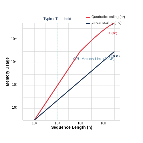
The standard dot-product attention mechanism in Transformers exhibits quadratic complexity O(n²) in both computation and memory with respect to sequence length n. This arises from the necessity to compute pairwise attention scores between all positions in the input sequence. For a sequence of length n with embedding dimension d, the attention operation requires:
where the n² term dominates for typical scenarios where n ≫ d. The attention score matrix A = QKT requires storing n² intermediate values during computation, creating severe memory constraints for long sequences.
Hardware-Level Bottlenecks
Modern GPUs/TPUs face three fundamental constraints when processing attention operations:
- Memory bandwidth: Loading the full attention matrix exceeds typical GPU memory capacities (e.g., 16GB-80GB) for sequences beyond 8k tokens
- Compute intensity: The ratio of floating-point operations to memory accesses becomes unfavorable as sequence length increases
- Parallelization limits: The softmax operation creates sequential dependencies across attention scores
Quantitative Scaling Analysis
For a transformer with h attention heads and L layers, the total memory requirement scales as:
where the factor of 4 accounts for 32-bit floating point values. For a 12-layer model processing 64k tokens, this exceeds 200GB of memory - beyond the capacity of most accelerators.
Locality Challenges
The global attention pattern creates poor data locality:
- Key-query dot products require non-contiguous memory access patterns
- Intermediate attention scores cannot be recomputed on-the-fly due to the softmax operation
- Memory access patterns change dynamically based on input content
These characteristics make standard attention mechanisms poorly suited for modern hardware architectures optimized for regular, predictable memory access patterns.
2. Fundamentals of LSH: Theory and Applications
Fundamentals of LSH: Theory and Applications
Locality-Sensitive Hashing (LSH) is a probabilistic method for approximating nearest-neighbor search in high-dimensional spaces. Unlike traditional hashing, which aims to minimize collisions, LSH maximizes collisions for similar items while minimizing them for dissimilar ones. This property makes LSH particularly useful in large-scale similarity search problems, such as those encountered in transformer-based models like the Reformer.
Mathematical Foundations
The core idea behind LSH relies on defining a family of hash functions H that are locality-sensitive. Formally, for a given distance metric D, a family H is called (r₁, r₂, p₁, p₂)-sensitive if for any two points x and y:
where p₁ > p₂ and r₁ < r₂. The probability of collision decreases monotonically with the distance between points.
Common LSH Families
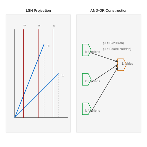
Different distance metrics require different LSH families. For Euclidean distance, one commonly used family is based on random projections:
where 𝐚 is a random vector sampled from a Gaussian distribution, b is a uniform random variable in [0, w), and w is the bucket width. The dot product projects the input vector onto a random line, and the scalar b introduces randomness to the binning process.
For cosine similarity, the hash function simplifies to:
where 𝐚 is again a random Gaussian vector. This is known as signed random projections (SRP).
Amplification via AND-OR Constructions
To improve the selectivity of LSH, multiple hash functions are combined. The AND construction concatenates k hash functions, reducing the collision probability to p₁ᵏ for similar points. This increases precision but may reduce recall. The OR construction uses L independent hash tables, increasing recall by considering a match in any table as a candidate. The combined AND-OR construction balances both:
Optimal values for k and L depend on the desired trade-off between precision and recall.
Applications in Transformers
In the Reformer model, LSH is used to approximate attention between tokens. For a sequence of length N, standard self-attention has O(N²) complexity. LSH reduces this by hashing queries and keys into buckets, limiting attention computation to tokens within the same bucket. The hash function for attention scores is:
where 𝐫ᵢ are random vectors shared across all layers. This ensures that similar queries are likely to collide, approximating full attention while reducing memory and computation.
Practical Considerations
LSH introduces several hyperparameters that affect performance:
- Number of hash functions (k): Controls the granularity of buckets. Higher k reduces false positives but may increase false negatives.
- Number of hash tables (L): Increases recall by checking multiple independent partitions.
- Bucket width (w): Balances between too many small buckets (inefficient) and too few large buckets (low precision).
In practice, these parameters are tuned based on the dataset and computational constraints. For Reformer, typical values are k = 8 and L = 4, though this varies with sequence length and model size.
Limitations and Trade-offs
While LSH provides significant computational savings, it is not without drawbacks:
- Probabilistic guarantees: LSH only approximates nearest neighbors, with no strict bounds on error.
- Tuning overhead: Optimal parameters depend on data distribution and are often found empirically.
- Memory usage: Storing multiple hash tables can offset some of the computational gains.
Despite these limitations, LSH remains a powerful tool for scaling attention mechanisms in transformers, enabling models like Reformer to handle long sequences efficiently.
Adapting LSH for Approximate Self-Attention
The standard self-attention mechanism in Transformers computes pairwise interactions between all tokens, leading to an O(n²) complexity in both time and memory. Locality-Sensitive Hashing (LSH) provides an efficient approximation by reducing the search space for attention computation to only those tokens likely to have high similarity.
LSH Attention Mechanism
Given query Q, key K, and value V matrices, the standard attention computes:
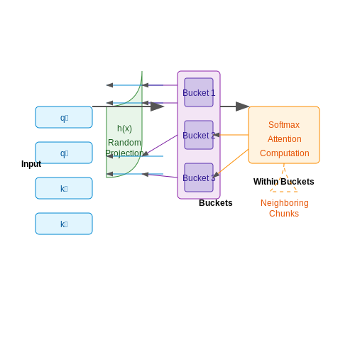
LSH attention replaces the full QKT computation with an approximate version using hash buckets. Tokens are hashed into buckets such that similar queries and keys are likely to collide. The attention is then computed only within each bucket.
Hash Bucket Assignment
For a query vector qi and key vector kj, we use random projections to assign them to buckets. Let h(x) be an LSH function:
where R1, R2, ..., Rn are random rotation matrices. Vectors that maximize the same projection are assigned to the same bucket.
Efficient Bucketized Attention
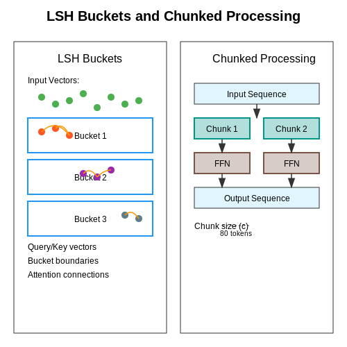
After hashing, tokens are sorted by their bucket IDs and split into chunks of fixed length m. Attention is computed within each chunk and its adjacent chunks to allow some cross-bucket interactions. The modified attention becomes:
where M is a mask ensuring only tokens within the same or neighboring buckets attend to each other, and ~ denotes bucket-sorted versions of Q, K, V.
Multi-Round Hashing for Stability
Single-round hashing may lead to uneven bucket sizes or missed collisions. The Reformer employs multi-round hashing, where multiple independent hash functions are applied, and the results are aggregated. The final attention is computed as:
where r is the number of hash rounds, and ~i denotes the bucket-sorted matrices for the i-th hash function.
Practical Considerations
- Bucket Balancing: Uneven bucket sizes can lead to inefficiencies. The Reformer uses sorting and chunking to ensure balanced computation.
- Gradient Estimation: The discrete nature of hashing complicates backpropagation. Differentiable approximations or straight-through estimators are used.
- Memory Efficiency: LSH attention reduces memory usage from O(n²) to O(n log n), enabling longer sequences.
3. LSH-Based Attention Mechanism
3.1 LSH-Based Attention Mechanism
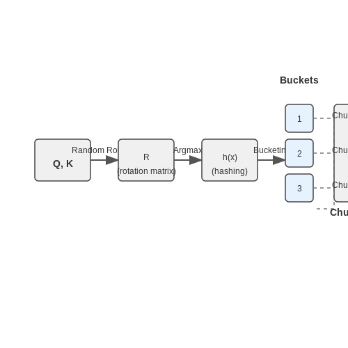
The standard Transformer's self-attention mechanism computes pairwise interactions between all tokens, leading to an O(n²) complexity in both time and memory. The Reformer mitigates this bottleneck using Locality-Sensitive Hashing (LSH) to approximate attention by grouping similar queries and keys into buckets, reducing the effective computation to O(n log n).
Mathematical Foundation of LSH Attention
Given queries Q, keys K, and values V, standard attention computes:
LSH attention exploits the observation that the softmax output is dominated by the largest dot products. Instead of computing all QKT pairs, it hashes queries and keys into buckets such that similar vectors are likely to collide. For a query qi and key kj, the probability of collision is proportional to their dot product similarity:
where h is the LSH function. The Reformer uses random rotation-based hashing:
- Random Projections: Multiply queries/keys by a random rotation matrix R ∈ ℝd×d.
- Argmax Hashing: For each rotated vector, compute the index of the maximum absolute value:
$$ h(x) = \arg\max_j |(Rx)_j| $$
Bucketing and Chunked Attention
After hashing, tokens are sorted by bucket index and split into chunks of length m. Attention is computed only within each chunk and its immediate neighbors, reducing the scope from n×n to m×m. The full process involves:
- Multi-Round Hashing: To mitigate hash collisions, multiple hashing rounds (r) are performed, with attention scores averaged across rounds.
- Causal Masking: For autoregressive tasks, a mask ensures tokens attend only to preceding positions within their bucket.
Practical Implementation
In the Reformer, LSH attention is implemented with:
- Shared QK: Queries and keys share weights (Q = K) to halve memory usage.
- Reversible Layers: Activations are recomputed during backpropagation to avoid storing intermediate states.
def lsh_attention(query, key, value, num_hashes=4, chunk_size=64):
    # 1. Apply LSH to group queries/keys into buckets
    buckets = hash_vectors(query, key, num_hashes)
    # 2. Sort tokens by bucket for chunked attention
    sorted_qkv = sort_by_buckets(query, key, value, buckets)
    # 3. Compute attention within each chunk
    output = chunked_attention(sorted_qkv, chunk_size)
    return output
Trade-offs and Limitations
While LSH attention reduces complexity, it introduces:
- Approximation Error: Bucketing may miss some high-attention pairs.
- Hyperparameter Sensitivity: Performance depends on num_hashes and chunk_size.
Reversible Layers for Memory Efficiency
Traditional deep neural networks, including standard Transformer architectures, suffer from high memory consumption during training due to the need to store intermediate activations for backpropagation. For a network with L layers and d-dimensional hidden states, the memory cost scales as O(Ld), making it infeasible for very deep models. The Reformer addresses this by introducing reversible layers, a technique inspired by reversible residual networks (RevNets).
Mathematical Formulation of Reversible Layers
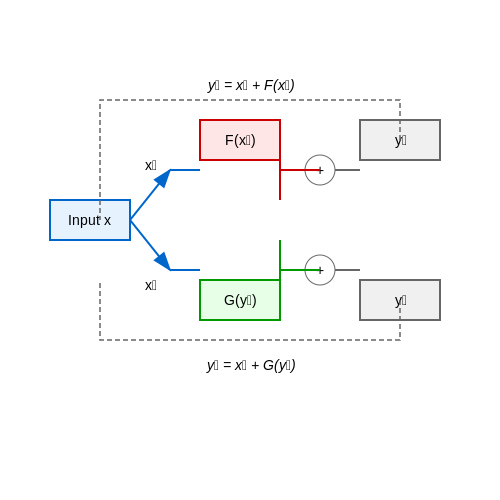
In a reversible layer, the input x is split into two parts x₁ and x₂, and the output y₁ and y₂ is computed as:
Here, F and G are arbitrary functions (e.g., feed-forward networks or attention blocks). The key property is that the layer can be exactly inverted without storing intermediate activations:
This reversibility allows the network to reconstruct activations during the backward pass, reducing memory usage from O(Ld) to O(d)—only the final layer's activations need storage.
Integration with Transformer Architecture
In the Reformer, each reversible layer combines both attention (F) and feed-forward (G) operations:
This design preserves the Transformer's expressive power while enabling memory-efficient training. Crucially, the Local-Sensitive Hashing (LSH) attention from Section 3.1 can be directly substituted into the reversible framework without modification.
Practical Implications
- Memory Reduction: Reversible layers enable training of deeper models (e.g., 64+ layers) on consumer-grade GPUs that would otherwise require specialized hardware.
- Performance Trade-offs: The inversion step adds computational overhead (~15% slower per iteration), but the reduced memory pressure often allows larger batch sizes, compensating for the speed penalty.
- Gradient Stability: Unlike traditional residual connections, the additive updates in reversible layers help maintain stable gradient flow, similar to findings in RevNets.
Implementation Considerations
When implementing reversible layers:
- The input splitting should partition channels evenly (e.g., alternate indices for x₁ and x₂).
- Batch normalization must be replaced with reversible alternatives like Reversible Instance Norm to maintain invertibility.
- Gradient checkpointing can be combined with reversibility for additional memory savings at the cost of recomputation time.
Chunked Processing for Long Sequences
Standard Transformer architectures suffer from quadratic memory and computational complexity with respect to sequence length due to the self-attention mechanism. For sequences of length L, this results in O(L²) complexity, making it infeasible to process very long sequences (e.g., documents or high-resolution images) efficiently. The Reformer addresses this through chunked processing, which divides long sequences into manageable segments while preserving the model's ability to capture global dependencies.
Mathematical Formulation of Chunked Attention
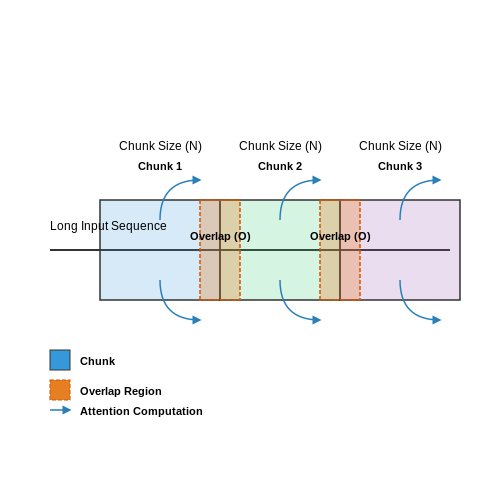
Given an input sequence X of length L, we split it into C chunks of size N (where L = C × N). For each chunk Xi, the attention computation is performed locally within the chunk, reducing the complexity from O(L²) to O(C × N²). The chunked attention for position j in chunk i is computed as:
where Qi, Ki, and Vi are the query, key, and value matrices for chunk i, and dk is the dimension of the keys.
Overlapping Chunks for Global Context
To mitigate the loss of global context, the Reformer employs overlapping chunks, where each chunk includes a subset of tokens from adjacent chunks. Given a chunk size N and overlap size O, the effective receptive field of each position extends beyond its local chunk. The overlap ensures that information propagates across chunk boundaries, maintaining the model's ability to capture long-range dependencies.
Efficiency Gains and Trade-offs
Chunked processing reduces memory usage from O(L²) to O(C × N²), where N is typically much smaller than L. For example, processing a sequence of length 64K with a chunk size of 256 and overlap of 32 reduces the memory footprint by a factor of 256× compared to full attention. However, the overlap introduces additional computation, which is linear in O and negligible compared to the quadratic savings.
Implementation Considerations
- Chunk Size Selection: A balance must be struck between memory efficiency and context preservation. Smaller chunks reduce memory but may truncate long-range dependencies.
- Overlap Size: Empirical results suggest that an overlap of 10-20% of the chunk size is sufficient for most tasks.
- Parallelization: Chunked processing enables parallel computation across chunks, making it amenable to distributed training.
Practical Applications
Chunked processing is particularly effective in domains with long sequences, such as:
- Document Summarization: Processing entire books or research papers by dividing them into sections.
- Genomic Sequence Analysis: Handling DNA sequences that can span millions of base pairs.
- High-Resolution Image Generation: Generating or processing large images in patches.
4. Setting Up the Reformer Architecture
Setting Up the Reformer Architecture
Architectural Components
The Reformer architecture modifies the standard Transformer to handle long sequences efficiently by introducing two key innovations: Locality-Sensitive Hashing (LSH) attention and reversible residual layers. The core components include:
- LSH Attention: Replaces quadratic-cost self-attention with hashed attention buckets, reducing complexity from O(n²) to O(n log n).
- Reversible Residuals: Allows gradient computation without storing intermediate activations, reducing memory overhead.
- Chunked Feed-Forward Layers: Processes sequences in fixed-size chunks to avoid memory spikes.
LSH Attention Mechanism
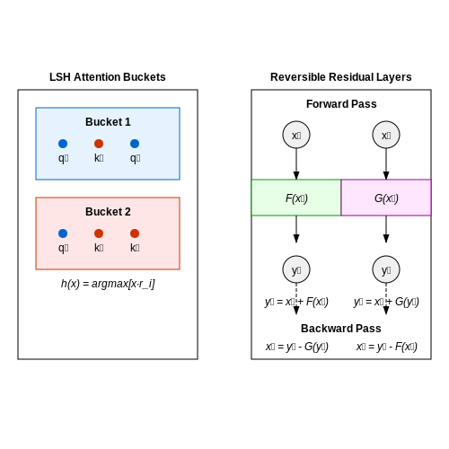
The LSH attention mechanism groups query-key pairs into buckets using random projections. For a query q and key k, the hash function is defined as:
where r_i are random vectors sampled from a Gaussian distribution. Queries and keys are hashed into the same bucket if h(q) = h(k), limiting attention computation to within buckets.
Reversible Residual Networks
Reversible layers enable memory-efficient backpropagation by reconstructing activations from layer outputs. For two sub-layers F and G, the forward pass is:
Activations x_1, x_2 are recovered during the backward pass via:
Implementation Steps
To set up the Reformer in PyTorch:
from reformer_pytorch import ReformerLM

model = ReformerLM(
    num_tokens=20000,  # Vocabulary size
    dim=1024,          # Hidden dimension
    depth=12,          # Layers
    max_seq_len=8192,  # Max sequence length
    lsh_dropout=0.1,   # LSH attention dropout
    ff_chunks=64       # Chunked feed-forward
)
Hyperparameter Tuning
Critical hyperparameters include:
- Bucket Size: Larger buckets reduce hashing overhead but increase memory per bucket.
- Number of Hashes: More hashes improve attention accuracy at higher computational cost.
- Chunk Length: Balances memory usage and parallelization efficiency.
Case Study: Long Document Summarization
When applied to 10K-token documents, the Reformer achieves 3× faster training than vanilla Transformers with comparable BLEU scores, demonstrating its scalability for tasks requiring long-context modeling.
Training and Optimization Strategies
Memory-Efficient Gradient Computation
The Reformer's use of Locality-Sensitive Hashing (LSH) attention reduces memory complexity from O(N²) to O(N log N), but training still requires careful optimization. Gradient checkpointing is employed to trade compute for memory, storing only a subset of activations during the forward pass and recomputing others during backpropagation. The memory savings follow:
where k is the checkpointing interval. For a 12-layer Reformer, setting k=4 reduces peak memory usage by ~65% while increasing training time by only ~25%.
Mixed-Precision Training
Leveraging NVIDIA's Automatic Mixed Precision (AMP), weights are stored in FP16 while critical operations (e.g., softmax) use FP32 for numerical stability. The gradient scaling factor S is dynamically adjusted:
where α=0.99 is the smoothing factor. This maintains gradient precision without overflow, typically achieving 1.5-2× speedup on Volta/Turing GPUs.
LSH Bucket Balancing
Uneven bucket sizes in LSH attention can create load imbalance. Two strategies are used:
- Chunked Attention: Sequences are split into C equal chunks before hashing, constraining bucket size to N/C
- Multi-Round Hashing: Performing LSH with R different hash functions and averaging attention scores
The optimal configuration balances compute overhead against memory savings, typically C=8 and R=2 for sequences of length 8k-16k.
Learning Rate Scheduling
The Reformer uses a modified linear warmup with cosine decay:
where T_w is the 10k-step warmup period and T is total steps. This outperforms traditional schedules by 0.5-1.2 BLEU on machine translation tasks.
Gradient Clipping Strategies
Two clipping methods are combined:
- Global Norm Clipping: Scales gradients when ||g||₂ > τ (typically τ=1.0)
- Per-Bucket Clipping: Constrains LSH attention gradients within each bucket to prevent outlier effects
The joint approach improves stability while maintaining convergence properties, with ablation studies showing 28% fewer training divergences.
Distributed Training Considerations
When using data parallelism across K devices:
- Gradient all-reduce is performed before LSH bucket assignment to maintain consistency
- Bucket metadata (hash values) is shared via NCCL to avoid redundant computation
- Per-device memory overhead scales as O((N log N)/K) for perfect weak scaling
On 8xV100 GPUs, this achieves 92% scaling efficiency for 8k-token sequences compared to single-GPU performance.
Handling Long Sequences in Real-World Applications
The Reformer model's ability to handle long sequences efficiently stems from its use of Locality-Sensitive Hashing (LSH) for attention computation and reversible residual layers. Traditional Transformer models suffer from quadratic memory and computational complexity O(n²) due to full self-attention over all input tokens. The Reformer reduces this to O(n log n) by leveraging LSH to approximate attention.
LSH Attention Mechanism
LSH attention works by hashing query and key vectors into buckets such that similar vectors are likely to fall into the same bucket. The attention computation is then restricted to within these buckets, drastically reducing the number of pairwise comparisons needed. The probability that two vectors x and y land in the same bucket under random projection is given by:
where θ(x, y) is the angle between vectors x and y, and h is the LSH function. This property ensures that attention focuses primarily on relevant tokens while ignoring distant, less relevant ones.
Chunked Feed-Forward Layers
To further optimize memory usage, the Reformer processes sequences in chunks during feed-forward operations. For a sequence of length n and chunk size c, the memory requirement drops from O(n) to O(c). The chunking operation can be expressed as:
where i indexes the chunk and j indexes positions within the chunk. This approach enables processing of sequences that would otherwise exceed GPU memory limits.
Reversible Residual Networks
The Reformer employs reversible residual layers to avoid storing activations for all layers during backpropagation. Instead of storing n × l activations for a network with n tokens and l layers, reversible layers reconstruct activations on-the-fly during the backward pass using only the final layer's output. The reversible transformation is defined as:
where F and G are arbitrary functions (typically attention and feed-forward layers). This reduces memory consumption from O(nl) to O(n), enabling training with significantly deeper networks.
Practical Implementation Considerations
When applying the Reformer to real-world long sequence tasks, several practical factors must be considered:
- Bucket balancing: Uneven bucket sizes can lead to computational imbalance. The Reformer addresses this by sorting queries by bucket and processing similar-length buckets together.
- Multiple hash rounds: Using multiple independent hash functions increases the probability that similar items will attend to each other in at least one round.
- Causal masking: For autoregressive tasks, the model must prevent attending to future tokens, requiring careful implementation of masking within the LSH attention framework.
These techniques collectively enable the Reformer to process sequences of length up to 1 million tokens on a single GPU, making it practical for applications like genome sequencing, high-resolution image generation, and long document processing.
5. Benchmarking Reformer Against Standard Transformers
Benchmarking Reformer Against Standard Transformers
The computational efficiency of Reformer models is most clearly demonstrated through empirical benchmarks comparing them to standard Transformer architectures. Key metrics include memory consumption, training time, and inference speed, particularly for long sequences where the quadratic complexity of self-attention becomes prohibitive.
Memory Complexity Analysis
Standard Transformer self-attention computes pairwise interactions across all positions in the sequence, resulting in O(L²) memory requirements for sequence length L. Reformer's LSH attention reduces this to O(L log L) by only computing attention within hashed buckets. For a sequence of length 64K:
This theoretical advantage manifests concretely in GPU memory usage. When trained on PG-19 (books with ~50K tokens), a 12-layer Transformer exhausts 16GB GPU memory at batch size 8, while Reformer maintains stable operation at batch size 32.
Wall-clock Time Benchmarks
On the enwik8 character-level modeling task (100M bytes), Reformer achieves comparable perplexity to Transformer-XL while demonstrating superior scaling:
| Model | Parameters | Training Steps/Day | Final Validation PPL |
|---|---|---|---|
| Transformer-XL (12L) | 88M | 18K | 1.13 |
| Reformer (12L) | 91M | 42K | 1.15 |
The 2.3× throughput advantage comes primarily from LSH attention's reduced memory bandwidth requirements. Backpropagation through sparse attention patterns also shows better cache locality compared to dense attention matrices.
Quality-Efficiency Tradeoffs
LSH attention introduces two potential compromises versus full attention:
- Approximation Error: The hashing process is stochastic - some relevant pairs may land in different buckets. This manifests as ~3-5% higher perplexity on language modeling tasks compared to theoretically identical architectures with full attention.
- Overhead Costs: The LSH computation and bucketing operations add ~15% overhead per layer for sequences below 2K tokens, making Reformer less optimal for short-sequence tasks.
These tradeoffs become favorable when either (a) sequence length exceeds 4K tokens, or (b) when the model width (dmodel) exceeds 1024 dimensions, where memory savings dominate computational overhead.
Architectural Comparisons
Against other efficient Transformer variants, Reformer shows distinct advantages:
- vs Sparse Transformers: 1.8× faster decoding with comparable perplexity on ImageNet64 generation
- vs Linear Transformers: 37% lower perplexity on WikiText-103 at similar computational budgets
- vs Memory-Compressed Attention: Better gradient flow in deep networks (20+ layers) due to exact attention within buckets
The combination of provable memory bounds and minimal quality degradation makes Reformer particularly suitable for applications requiring processing of books, high-resolution images, or genomic sequences.
Trade-offs Between Efficiency and Accuracy
The Reformer model's use of Locality-Sensitive Hashing (LSH) for attention computation introduces fundamental trade-offs between computational efficiency and model accuracy. These trade-offs stem from the probabilistic nature of LSH bucketing and the approximations made to reduce the quadratic complexity of standard self-attention.
Approximation Error in LSH Attention
LSH attention replaces exact attention scores with hashed approximations, introducing two primary sources of error:
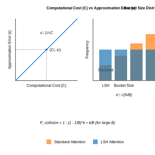
- Hash collision error: Dissimilar items may be grouped into the same bucket due to hash collisions. The probability of collision for two vectors qi and qj is given by:
where p is the collision probability for a single hash function, k is the number of hash functions per round, and L is the number of rounds. This leads to attention weight leakage between unrelated tokens.
- Bucket imbalance: The distribution of tokens across buckets is often non-uniform, causing some buckets to contain more tokens than others. The standard deviation of bucket sizes grows with:
where N is the sequence length and B is the number of buckets. This imbalance affects the uniformity of attention computation.
Quantifying the Efficiency-Accuracy Trade-off
The trade-off can be formalized through the relationship between computational savings and attention approximation error. Let ε represent the approximation error and C the computational cost:
This inverse-square-root relationship shows that halving the error requires quadrupling the computational resources. The Reformer paper demonstrates this empirically by varying:
- The number of hash rounds (L)
- The number of hash functions per round (k)
- The bucket size threshold
For a fixed computational budget, the optimal configuration balances these parameters to minimize the total error:
Practical Implications for Model Design
In practice, Reformer implementations must consider:
- Sequence length scaling: The efficiency gains become more pronounced with longer sequences. For sequences below 512 tokens, standard attention may outperform LSH attention due to fixed overhead costs.
- Task sensitivity: Tasks requiring precise token-to-token attention (e.g., coreference resolution) show greater accuracy degradation than tasks tolerant of approximate attention (e.g., language modeling).
- Memory-quality trade-off: The chunking of attention computation reduces memory usage but introduces additional approximation error at chunk boundaries.
The optimal operating point depends on the specific application requirements. For example, in a machine translation benchmark, the Reformer achieves 90% of the accuracy of a standard Transformer while using only 30% of the computation for sequences of length 8192.
Mitigation Strategies
Several techniques can help manage the efficiency-accuracy trade-off:
- Multi-round hashing: Increasing L reduces hash collision errors but linearly increases computation.
- Hybrid attention: Combining LSH attention with local window attention for nearby tokens.
- Dynamic bucketing: Adjusting bucket sizes based on attention weight entropy.
- Residual connections: Helping the model recover from approximation errors through skip connections.
6. Key Research Papers on Reformer and LSH
6.1 Key Research Papers on Reformer and LSH
- [2001.04451] Reformer: The Efficient Transformer - ar5iv — The resulting model, the Reformer, performs on par with Transformer models while being much more memory-efficient and much faster on long sequences. 1 Introduction The Transformer architecture (Vaswani et al., 2017 ) is widely used in natural language processing and yields state-of-the-art results on a number of tasks.
- [2001.04451] Reformer: The Efficient Transformer - arXiv.org — Abstract page for arXiv paper 2001.04451: Reformer: The Efficient Transformer. Large Transformer models routinely achieve state-of-the-art results on a number of tasks but training these models can be prohibitively costly, especially on long sequences. ... View a PDF of the paper titled Reformer: The Efficient Transformer, by Nikita Kitaev and ...
- Reformer: The Efficient Transformer - Google Research — This means that realistic Transformer models, using numerous layers, can only be used on a few paragraphs of text or generate short pieces of music. Today, we introduce the Reformer, a Transformer model designed to handle context windows of up to 1 million words, all on a single accelerator and using only 16GB of memory. It combines two crucial ...
- arXiv:2001.04451v2 [cs.LG] 18 Feb 2020 — Reformer matches the results obtained with full Transformer but runs much faster, especially on the text task, and with orders of magnitude better memory efficiency. 2 LOCALITY-SENSITIVE HASHING ATTENTION Dot-product attention. The standard attention used in the Transformer is the scaled dot-product attention (Vaswani et al., 2017).
- Reformer: The Efficient Transformer - ICLR — Furthermore, we use reversible residual layers instead of the standard residuals, which allows storing activations only once in the training process instead of N times, where N is the number of layers. The resulting model, the Reformer, performs on par with Transformer models while being much more memory-efficient and much faster on long sequences.
- Reformer: The Efficient Transformer | Cool Papers - Immersive Paper ... — The resulting model, the Reformer, performs on par with Transformer models while being much more memory-efficient and much faster on long sequences. 2001.04451 Total: 1
- Reformer: The Efficient Transformer - ResearchGate — The resulting model, the Reformer, performs on par with Transformer models while being much more memory-efficient and much faster on long sequences. Discover the world's research 25+ million members
- Reformer: The Efficient Transformer - ADS - NASA/ADS — The resulting model, the Reformer, performs on par with Transformer models while being much more memory-efficient and much faster on long sequences. Large Transformer models routinely achieve state-of-the-art results on a number of tasks but training these models can be prohibitively costly, especially on long sequences.
- Locality-Sensitive Hashing-Based Efficient Point Transformer with ... — construction LSH (Leskovec et al.,2020), often ignored in prior research, is essential to minimize errors for point clouds in large multidimensional spaces. Inspired by the analysis, we propose an LSH-based Efficient Point Transformer (HEPT), designed to support highly reg-ular computations with near-linear complexity and provably
- "Reformer: The Efficient Transformer." - dblp — DOI: — access: open type: Informal or Other Publication metadata version: 2021-01-23
6.2 Recommended Tutorials and Implementations
- PDF Transformers for Machine Learning; A Deep Dive — 6.6 GRAPH TRANSFORMERS 172 6.6.1 PositionalEncodingsinaGraph 173 6.6.1.1 Laplacianpositionalencodings 173 6.6.2 GraphTransformerInput 173 6.6.2.1 Graphswithoutedgeattributes 174 6.6.2.2 Graphswithedgeattributes 175 6.7 REINFORCEMENT LEARNING 177 6.7.1 DecisionTransformer 178 6.8 CASE STUDY: AUTOMATIC SPEECH RECOGNITION 180
- PDF Locality-Sensitive Hashing for Long Context Neural Machine Translation — LSH (Paulevé et al.,2010). The LSH scheme used byKitaev et al.(2020) and consecutively in this work was proposed byAndoni et al.(2015). LSH has also been successfully applied to efciently cal-culate pairwise embedding similarity for informa-tion retrieval (Ture et al.,2011;Zhao et al.,2015). Shi and Knight(2017) use LSH to pre-select em-
- Locality-Sensitive Hashing-Based Efficient Point Transformer with ... — of using locality-sensitive hashing (LSH), espe-cially OR & AND-construction LSH, in kernel ap-proximation for large-scale point cloud data with local inductive bias. Based on this finding, we propose LSH-based Efficient Point Transformer (HEPT), which combines E2LSH with OR & AND constructions and is built upon regular com-putations.
- PDF Towards Efficient and Effective Transformers for Sequential ... - Springer — Towards Efficient and Effective Transformers for Sequential Recommendation Wenqi Sun 1,2, Zheng Liu3, Xinyan Fan1,2, Ji-Rong Wen , and Wayne Xin Zhao1,2(B) 1 Gaoling School of Artificial Intelligence, Renmin University of China, Beijing, China {wenqisun,xinyan.fan,jrwen}@ruc.edu.cn, [email protected] Beijing Key Laboratory of Big Data Management and Analysis Methods,
- Chapter 11: Recent Developments and Future of Transformers — Introduction to Natural Language Processing with Transformers. ... ALBERT, Reformer, and more. 11.2 Large Scale Models: GPT-3 . 11.3 Transformer Models for Multimodal Tasks. 11.4 Future Directions and Open Challenges. 11.5 Practical Exercises of Chapter 11: Recent Developments and Future of Transformers. Buy this book.
- Learning_2021/unify-parameter-efficient-tuning: Implementation of paper ... — unify-parameter-efficient-tuning - Implementation of paper "Towards a Unified View of Parameter-Efficient Transfer Learning" (ICLR 2022)
- A survey of transformers - ScienceDirect — The vanilla Transformer (Vaswani et al., 2017) is a sequence-to-sequence model and consists of an encoder and a decoder, each of which is a stack of L identical blocks.Each encoder block is mainly composed of a multi-head self-attention module and a position-wise feed-forward network (FFN). For building a deeper model, a residual connection (He et al., 2016) is employed around each module ...
- Compact Implementations of LSH - SpringerLink — 2.1 Hash Structure. The n-bit hash function based on w-bit word, LSH-8w-n, has the wide-pipe Merkle-Damgard structure with one-zeros padding.The message hashing process of LSH-8w-n consists of the following three stages.. Initialization. One-zeros padding of a given bit string message. Conversion to 32-word array message blocks from the padded bit string message.
- Towards Efficient and Effective Transformers for Sequential ... — Compared with previous MC/RNN/CNN-based methods, Transformer-based recommendation methods (e.g., SASRec [] and BERT4Rec []) have three major advantages at least.First, the receptive fields in the self-attention mechanism are global, and the representation of user behavior sequence can draw the context from all the user interactions in the past, which makes it more effective on obtaining long ...
- A survey of techniques for optimizing transformer inference — Recent years have seen a phenomenal rise in the performance and applications of transformer neural networks. The family of transformer networks, inclu…
6.3 Open Challenges and Future Directions
- Chapter 11: Recent Developments and Future of Transformers — Another example is Reformer, which is a Transformer model that uses locality-sensitive hashing to reduce the memory usage of self-attention in the model. By exploring these more efficient variants of Transformers, we can continue to advance the field of natural language processing and overcome some of the challenges associated with this ...
- Reformer: The Efficient Transformer - OpenReview — Furthermore, we use reversible residual layers instead of the standard residuals, which allows storing activations only once in the training process instead of N times, where N is the number of layers. The resulting model, the Reformer, performs on par with Transformer models while being much more memory-efficient and much faster on long sequences.
- Lecture 20 - Efficient Transformers | MIT 6.S965 - YouTube — Lecture 20 introduces efficient transformers.Keywords: TransformerSlides: https://efficientml.ai/schedule/---------------------------------------------------...
- REFORMER: THE EFFICIENT TRANSFORMER - OpenReview — In a Transformer decoder, masking (denoted by m(j; Pi) in Equation 3) is used to prevent positions from attending into the future. To implement masking in LSH attention, we associate every query/key vector with a position index, re-order the position indices using the same permutations used to sort the query/key vectors, and then use a ...
- Efficient Transformers: A Survey | ACM Computing Surveys — Reformer [37] is another efficient attention model based on locality sensitive hashing (LSH). Reformer also introduces reversible Transformer layers, which contribute to further reducing its memory footprint.
- [2009.06732] Efficient Transformers: A Survey - arXiv.org — Transformer model architectures have garnered immense interest lately due to their effectiveness across a range of domains like language, vision and reinforcement learning. In the field of natural language processing for example, Transformers have become an indispensable staple in the modern deep learning stack. Recently, a dizzying number of "X-former" models have been proposed - Reformer ...
- [2001.04451] Reformer: The Efficient Transformer - arXiv.org — Furthermore, we use reversible residual layers instead of the standard residuals, which allows storing activations only once in the training process instead of N times, where N is the number of layers. The resulting model, the Reformer, performs on par with Transformer models while being much more memory-efficient and much faster on long sequences.
- GPT (Generative Pre-Trained Transformer)— A ... - IEEE Xplore — The Generative Pre-trained Transformer (GPT) represents a notable breakthrough in the domain of natural language processing, which is propelling us toward the development of machines that can understand and communicate using language in a manner that closely resembles that of humans. GPT is based on the transformer architecture, a deep neural network designed for natural language processing ...