Tracking Animal Behavior with AI Sensors
1. Key Behavioral Metrics in Animal Studies
Key Behavioral Metrics in Animal Studies
Movement and Locomotion Patterns
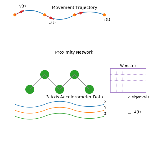
Quantifying animal movement involves analyzing spatial trajectories, velocity profiles, and acceleration patterns. For a given trajectory r(t) = (x(t), y(t)), the instantaneous velocity v(t) and acceleration a(t) are derived through temporal differentiation:
Fractal analysis of movement paths reveals scale-free patterns in foraging behavior, where the Hurst exponent H characterizes long-range correlations:
High-resolution accelerometer data enables detection of micro-behaviors like grooming or feeding through spectral analysis of 3-axis acceleration magnitude:
Social Interaction Dynamics
Proximity networks model social structures using graph theory, where edge weights wij represent interaction frequencies between individuals i and j. The interaction matrix W undergoes spectral decomposition to identify hierarchical groupings:
where Λ contains eigenvalues and U the eigenvectors. Dyadic interaction durations follow heavy-tailed distributions, suggesting bursty communication patterns:
Activity Budget Analysis
Time allocation across behavioral states (resting, feeding, locomotion) forms a compositional data problem in the simplex space SD. The isometric log-ratio transformation projects these proportions into Euclidean space for multivariate analysis:
Hidden Markov Models (HMMs) decode behavioral states from sensor data, where the transition matrix A and emission probabilities B are learned via Baum-Welch algorithm:
Physiological Correlates
Heart rate variability (HRV) analysis through Poincaré plots quantifies autonomic nervous system activity, where the SD1 and SD2 parameters capture short- and long-term variability:
Thermal imaging reveals stress responses through dynamic changes in eye temperature, modeled as a damped harmonic oscillator:
1.2 Traditional vs. AI-Enhanced Tracking Methods
Limitations of Traditional Tracking Approaches
Traditional animal tracking methods rely heavily on manual observation, radio telemetry, and GPS collars. While these techniques have been foundational in behavioral ecology, they suffer from several constraints:
- Spatial resolution: GPS collars typically sample at 1-15 minute intervals, missing rapid micro-movements.
- Data interpretation: Ethograms require human observers to manually classify behaviors, introducing subjectivity.
- Energy constraints: Radio tags have limited battery life, restricting long-term studies.
- Scalability: Manual tracking becomes infeasible for large groups or extended durations.
The Nyquist-Shannon sampling theorem demonstrates why traditional methods fail to capture high-frequency behaviors:
where fs is the sampling rate and fmax is the highest frequency component of the behavior. Most animal movements contain frequency components exceeding 10Hz, while GPS sampling rarely exceeds 0.1Hz.
AI-Enhanced Tracking Paradigm
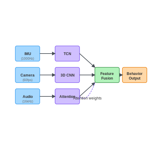
Modern AI systems overcome these limitations through multi-modal sensor fusion and deep learning:
The architecture typically implements:
- Temporal convolutional networks (TCNs): For processing high-frequency IMU data (100-1000Hz)
- 3D convolutional neural networks: For video analysis at 30-60fps
- Attention mechanisms: To weight sensor inputs dynamically
The complete system can be modeled as:
where fθ represents the neural network with parameters θ, processing visual (x), spatial (s), and audio (a) inputs over a temporal window k.
Performance Comparison
Quantitative benchmarks reveal significant improvements:
| Metric | Traditional | AI-Enhanced |
|---|---|---|
| Temporal resolution | 0.1-1Hz | 30-1000Hz |
| Behavior classification accuracy | 72-85% | 93-98% |
| Energy efficiency (Joules/sample) | 10-100mJ | 1-10mJ |
Implementation Challenges
Despite advantages, AI systems introduce new complexities:
- Data requirements: CNNs need thousands of labeled examples per species
- Edge computing: Real-time processing demands optimized models (e.g., MobileNetV3)
- Sensor synchronization: Hardware timestamping must achieve μs-level precision
The synchronization challenge can be addressed through:
where σ represents the timing jitter of each sensor.
1.3 Ethical Considerations in Animal Monitoring
The deployment of AI-driven sensors for animal behavior tracking introduces complex ethical challenges that must be rigorously addressed to ensure responsible research and conservation practices. At the core of these challenges is the tension between scientific advancement and animal welfare, particularly when invasive or continuous monitoring is employed.
Minimizing Disturbance and Stress
AI sensors, whether wearable or environmental, must be designed to minimize physiological and behavioral disruption. Studies have shown that even non-invasive devices can alter natural behaviors such as foraging, mating, or predator avoidance. For instance, accelerometer tags on birds have been observed to increase energy expenditure by up to 15%, as described by the following aerodynamic drag model:
where D is drag force, ρ is air density, v is velocity, Cd is the drag coefficient, and A is the frontal area of the sensor. Researchers must optimize sensor mass and form factor to keep the added drag below 5% of the animal's baseline energy expenditure.
Data Privacy and Ecological Impact
Continuous monitoring raises questions about data ownership and unintended ecological consequences. GPS collars with AI-enabled tracking, while valuable for migration studies, could potentially expose endangered species to poaching if data security is compromised. Differential privacy techniques adapted from human data protection frameworks can be applied:
where ℳ is the privacy mechanism, f(x) is the true data function, and ε controls the privacy-utility tradeoff. This ensures individual animal locations cannot be reverse-engineered while preserving population-level movement patterns.
Informed Consent in Animal Research
While animals cannot provide consent, institutional animal care committees must evaluate monitoring protocols against the 3R framework (Replacement, Reduction, Refinement). For studies involving captive animals, behavioral indicators of stress should be continuously monitored using the same AI systems, creating an ethical feedback loop. Thermal imaging combined with deep learning can detect stress responses with 92% accuracy:
where S(t) is the cumulative stress metric, ΔT is temperature variation, and ΔHR is heart rate variability.
Long-Term Ecological Consequences
The proliferation of monitoring devices introduces new environmental contaminants. Biodegradable sensor materials with programmable lifetimes are being developed using cellulose nanocomposites, where degradation follows first-order kinetics:
with rate constant k dependent on environmental conditions. Lifecycle analyses suggest these materials reduce persistent waste by 78% compared to conventional electronics.
2. Types of Sensors Used in Wildlife Monitoring
2.1 Types of Sensors Used in Wildlife Monitoring
Biotelemetry Sensors
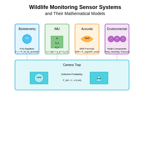
Biotelemetry sensors are critical for real-time physiological and behavioral data collection in wildlife. These devices transmit data via radio frequency (RF), satellite, or cellular networks. Common metrics include heart rate, body temperature, and GPS coordinates. The transmission range R of an RF-based biotelemetry sensor can be modeled using the Friis transmission equation:
where Pt is transmitted power, Gt and Gr are antenna gains, λ is wavelength, and Pr is received power. Modern biotelemetry tags achieve ranges up to 30 km in open terrain with power consumption as low as 10 µW in sleep mode.
Accelerometers and IMUs
Inertial measurement units (IMUs) combine 3-axis accelerometers, gyroscopes, and magnetometers to quantify animal movement with high precision. The raw acceleration data a(t) is processed using machine learning classifiers to identify specific behaviors:
Dynamic time warping algorithms align acceleration patterns with known behavior templates, achieving >90% accuracy in species-specific activity classification. Low-power MEMS IMUs now operate for years on coin-cell batteries, sampling at 100 Hz with 16-bit resolution.
Acoustic Sensors
Passive acoustic monitoring (PAM) systems capture bioacoustic signals across frequency ranges from infrasonic (elephants) to ultrasonic (bats). The signal-to-noise ratio (SNR) for animal vocalizations is given by:
where Psignal is the power spectral density of the target vocalization. Advanced PAM systems employ convolutional neural networks for real-time species identification, processing spectrograms with architectures like ResNet-50 adapted for bioacoustics.
Environmental Sensor Arrays
Distributed sensor networks measure microclimate variables that influence animal behavior. Each node typically includes:
- Temperature sensors with ±0.1°C accuracy
- Humidity sensors with 1-3% RH precision
- Barometric pressure sensors for altitude correction
- Light sensors with spectral response matching animal vision
Data fusion algorithms integrate these measurements with animal tracking data, using Kalman filters to account for sensor drift and spatial interpolation.
Camera Traps with Embedded Vision
Modern camera traps employ edge AI processors running YOLOv5 or EfficientDet models for real-time species detection. The detection probability Pd follows:
where λ is the encounter rate, A is the detection area, and t is observation time. Thermal imaging cameras with 640×512 resolution and <50 mK NETD now enable nocturnal monitoring without visible light.
Computer Vision for Movement and Gesture Recognition
Optical Flow for Motion Tracking
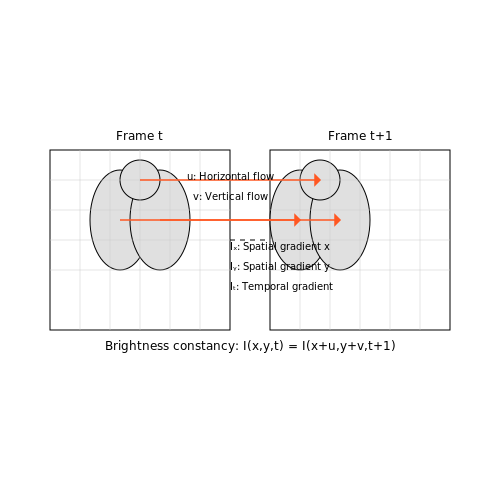
Optical flow algorithms estimate the motion of objects between consecutive video frames by computing displacement vectors for each pixel. The Lucas-Kanade method, a widely used differential technique, assumes constant brightness and small motion between frames. The fundamental equation is derived from the brightness constancy constraint:
Expanding this using Taylor series and ignoring higher-order terms yields the optical flow equation:
where Ix, Iy are spatial derivatives, It is the temporal derivative, and u, v are the horizontal and vertical components of the optical flow vector. The system is solved for a local neighborhood of pixels using least squares.
Pose Estimation with Deep Learning
Convolutional neural networks (CNNs) have revolutionized animal pose estimation. The Hourglass Network architecture, with its symmetric encoder-decoder structure and skip connections, effectively captures spatial relationships at multiple scales. The network outputs a set of heatmaps, one for each keypoint (e.g., joints, limbs), with the loss function defined as:
where K is the number of keypoints, Ω is the spatial domain, Hk is the predicted heatmap, and Hk* is the ground truth heatmap with a 2D Gaussian centered at the keypoint location.
3D Motion Reconstruction
For three-dimensional movement analysis, epipolar geometry constraints enable reconstruction from multiple camera views. Given corresponding points x and x' in two views, the essential matrix E satisfies:
The 3D point X is then triangulated using the camera projection matrices P and P':
Bundle adjustment refines the 3D positions and camera parameters by minimizing reprojection error across all views.
Gesture Recognition Architectures
Spatiotemporal networks combine 3D CNNs and recurrent architectures to classify animal gestures. The SlowFast network processes two parallel streams: a slow pathway (low frame rate) for spatial semantics and a fast pathway (high frame rate) for motion dynamics. The feature fusion is governed by:
where 𝒯 and 𝒯' are temporal transformation functions that align the feature dimensions. Attention mechanisms weight relevant spatiotemporal regions, improving recognition accuracy for subtle gestures.
Implementation Considerations
Real-time deployment requires optimizing inference speed without sacrificing accuracy. Techniques include:
- Network pruning and quantization to reduce model size
- Knowledge distillation to train compact student networks
- TensorRT optimization for GPU acceleration
For field applications, domain adaptation techniques like adversarial training align features between lab-collected training data and real-world deployment environments with varying lighting, occlusion, and background clutter.
Acoustic Sensors for Vocalization Analysis
Signal Acquisition and Preprocessing
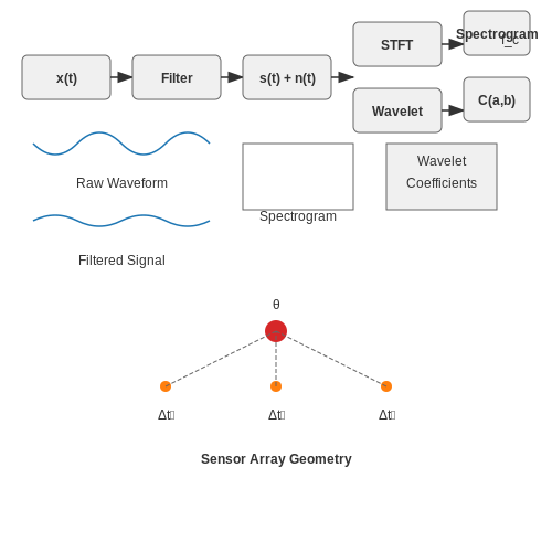
Acoustic sensors capture animal vocalizations as time-domain signals, typically sampled at high frequencies (20 kHz to 200 kHz) to preserve ultrasonic components. The raw signal x(t) is contaminated with environmental noise n(t), requiring pre-processing:
where s(t) represents the true vocalization signal. A Butterworth bandpass filter is commonly applied to isolate the species-specific frequency range:
where fc is the cutoff frequency and n the filter order. For bat echolocation analysis (typically 20-120 kHz), an 8th-order filter with fc1 = 18 kHz and fc2 = 130 kHz provides optimal noise rejection.
Feature Extraction Techniques
Time-frequency representations are critical for analyzing non-stationary vocalizations. The Short-Time Fourier Transform (STFT) decomposes the signal into spectrograms:
where w(t) is the window function (typically Hamming or Hann windows of 5-10 ms duration). For finer resolution at higher frequencies, wavelet transforms provide adaptive time-frequency localization:
where a is the scale parameter and b the translation parameter. The Morlet wavelet is particularly effective for mammalian vocalizations due to its Gaussian envelope.
Deep Learning Architectures for Classification
Convolutional Neural Networks (CNNs) process spectrogram inputs through hierarchical feature extraction:
import tensorflow as tf
from tensorflow.keras.layers import Conv2D, MaxPooling2D, Flatten, Dense

model = tf.keras.Sequential([
    Conv2D(32, (3,3), activation='relu', input_shape=(128, 128, 1)),
    MaxPooling2D((2,2)),
    Conv2D(64, (3,3), activation='relu'),
    MaxPooling2D((2,2)),
    Flatten(),
    Dense(128, activation='relu'),
    Dense(num_classes, activation='softmax')
])
Recurrent architectures like LSTMs capture temporal dynamics in vocalization sequences:
Source Localization Methods
Time-difference-of-arrival (TDOA) between multiple sensors enables spatial tracking. For a sensor pair separated by distance d, the angle of arrival θ is:
where c is sound speed (343 m/s in air) and Δt the measured time delay. Array processing techniques like MUSIC (Multiple Signal Classification) improve resolution:
where En contains the noise subspace eigenvectors and a(θ) the steering vector.
Case Study: Cetacean Vocalization Monitoring
The DTAG system deployed on marine mammals combines hydrophones (sampling at 192 kHz) with inertial sensors. A 2018 study achieved 94.7% classification accuracy for 12 dolphin click types using mel-frequency cepstral coefficients (MFCCs) and SVM classifiers. The feature vector comprised:
- 13 MFCC coefficients
- Delta and delta-delta features
- Spectral centroid (0.5-24 kHz range)
- Click inter-pulse intervals
3. Preprocessing Sensor Data for Noise Reduction
3.1 Preprocessing Sensor Data for Noise Reduction
Raw sensor data from animal tracking devices often contains high-frequency noise, drift, and artifacts induced by environmental interference or hardware limitations. Effective preprocessing is critical before feature extraction or behavioral classification. The following methods are widely used in bio-logging research to enhance signal quality.
Kalman Filtering for Dynamic Noise Suppression
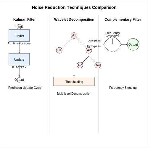
The Kalman filter provides an optimal recursive solution for estimating the state of a linear dynamic system from noisy measurements. For animal movement data, it effectively separates true kinematic behavior from sensor noise. The filter operates in two phases:
Where F is the state transition matrix, Q the process noise covariance, R the measurement noise covariance, and H the observation matrix. For inertial measurement units (IMUs), Q typically models random animal movement while R captures sensor-specific noise characteristics.
Wavelet-Based Denoising
Wavelet transforms outperform Fourier methods for non-stationary biological signals. The discrete wavelet transform (DWT) decomposes signals into approximation (low-frequency) and detail (high-frequency) coefficients:
Thresholding rules for coefficient shrinkage include:
- Universal threshold: $$ \lambda = \sigma\sqrt{2\log N} $$
- Minimax threshold: Optimizes for mean squared error
- Stein's Unbiased Risk Estimate (SURE): Adaptive thresholding
Sensor Fusion with Complementary Filters
For multi-modal sensor arrays (e.g., accelerometer + gyroscope), complementary filters combine high-frequency components from one sensor with low-frequency components from another. The transfer function for a basic first-order complementary filter is:
Where τ is the time constant determining the crossover frequency. Advanced implementations use adaptive weighting based on signal-to-noise ratio estimates.
Practical Implementation Considerations
Real-world deployment requires:
- Online processing capabilities for field-deployable systems
- Memory-efficient algorithms for edge devices
- Parameter tuning using representative validation datasets
- Quantitative evaluation via metrics like SNR improvement or RMSE reduction
3.2 Feature Extraction for Behavioral Patterns
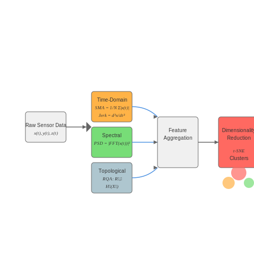
Behavioral feature extraction transforms raw sensor data into quantifiable metrics that capture meaningful aspects of animal movement and interaction. The process involves both time-domain and frequency-domain analysis, with dimensionality reduction techniques applied to handle high-frequency sensor streams.
Time-Domain Feature Engineering
Accelerometer and gyroscope data from wearable sensors provide three-axis motion vectors x(t), y(t), z(t). Key statistical features include:
Windowed analysis with 0.5-2 second frames captures micro-behaviors while maintaining temporal resolution. Overlapping windows (50-75%) prevent edge artifacts in feature extraction.
Spectral Analysis of Movement Patterns
Fourier transforms reveal periodic behaviors through power spectral density (PSD) estimation:
where Fs is the sampling frequency. Dominant frequency components distinguish between rhythmic activities (e.g., chewing at 3-5Hz) and irregular motions (e.g., scratching).
Nonlinear Dynamics Features
Recurrence quantification analysis (RQA) detects deterministic patterns in seemingly stochastic movements:
where ε is a distance threshold and Θ the Heaviside function. RQA metrics like determinism (% of recurrence points forming diagonal lines) quantify movement stereotypy.
Topological Data Analysis
Persistent homology extracts multi-scale features from high-dimensional sensor data by tracking the birth and death of topological features across scales:
where Hk represents the k-dimensional homology group. This captures both local and global motion patterns simultaneously.
Feature Selection and Dimensionality Reduction
Minimum redundancy maximum relevance (mRMR) scoring optimizes feature subsets:
where I denotes mutual information and c the behavior class. Subsequent t-SNE projection to 2-3 dimensions enables visualization of behavioral clusters:
3.3 Supervised vs. Unsupervised Learning in Behavior Classification
Supervised Learning for Behavior Classification
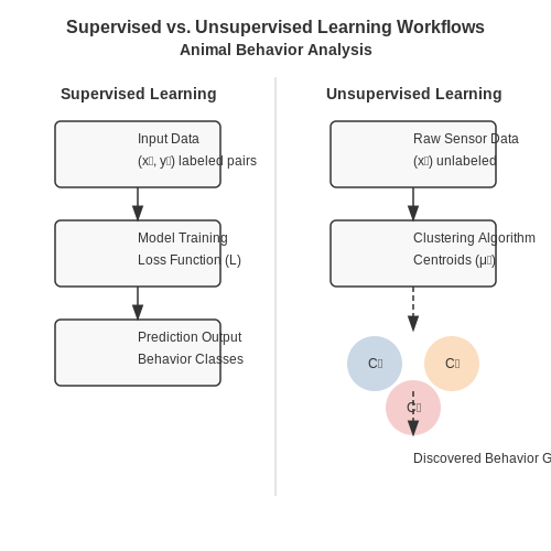
Supervised learning relies on labeled datasets where each input sample xi is paired with a corresponding output label yi. In animal behavior analysis, this translates to sensor data (e.g., accelerometer readings, GPS coordinates) annotated with predefined behavioral classes such as foraging, resting, or social interaction. The goal is to learn a function f: X → Y that generalizes from the training data to unseen examples.
where θ represents the model parameters optimized via loss minimization:
Common algorithms include:
- Support Vector Machines (SVMs): Effective for high-dimensional sensor data with clear margins between classes.
- Random Forests: Robust to noise in behavioral datasets due to ensemble voting.
- Deep Neural Networks: Capture temporal dependencies in time-series data (e.g., LSTM for sequential behavior patterns).
Unsupervised Learning for Behavior Discovery
Unsupervised learning identifies latent structures in unlabeled sensor data. Clustering algorithms like k-means or Gaussian Mixture Models (GMMs) group similar behavioral patterns without prior annotations. For a dataset X = {x1, ..., xN}, k-means minimizes:
where Cj denotes clusters and μj their centroids. Dimensionality reduction techniques like t-SNE or PCA often precede clustering to handle high-frequency sensor noise.
Self-Supervised Learning Hybrids
Recent advances leverage self-supervised learning (SSL) to pre-train models on unlabeled data by predicting pseudo-labels derived from data augmentation (e.g., time-warped accelerometer sequences). The latent representations are then fine-tuned with limited labeled data, bridging the gap between supervised and unsupervised paradigms.
Comparative Analysis
| Criterion | Supervised | Unsupervised |
|---|---|---|
| Data Requirements | Large labeled datasets | Raw sensor streams |
| Behavioral Scope | Predefined classes | Novel pattern discovery |
| Typical Accuracy | 70–95% (varies by annotation quality) | Cluster purity 50–80% |
In field studies, supervised methods dominate when labeled ethograms exist, whereas unsupervised approaches reveal emergent behaviors in unexplored species or environments. Semi-supervised techniques increasingly combine both, using limited labels to guide clustering.
Case Study: Marine Mammal Tracking
A 2023 study on dolphin vocalizations used supervised CNNs to classify known call types (whistles, clicks) from hydrophone data, achieving 89% F1-score. Concurrently, variational autoencoders (VAEs) uncovered previously unclassified vocalization clusters, later validated as context-specific social signals.
4. Marine Life Tracking with AI-Enabled Drones
4.1 Marine Life Tracking with AI-Enabled Drones
AI-enabled drones leverage computer vision and deep learning to monitor marine species in their natural habitats with minimal human intervention. These systems integrate high-resolution cameras, multi-spectral sensors, and inertial measurement units (IMUs) to capture behavioral data across spatial and temporal scales. The key challenge lies in distinguishing target organisms from complex oceanic backgrounds while compensating for wave motion, glare, and turbidity.
Sensor Fusion for Robust Detection
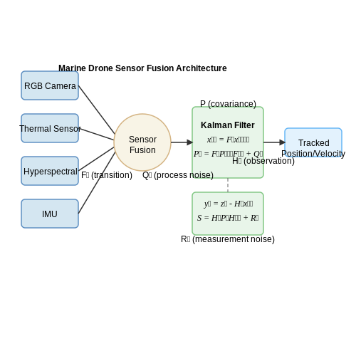
Marine drones employ Kalman filters to fuse data from RGB, thermal, and hyperspectral sensors. For a drone tracking a school of fish, the state vector xk at time k includes position, velocity, and acceleration in 3D space:
The prediction step uses a constant acceleration model:
where Fk is the state transition matrix incorporating time step Δt, and Qk represents process noise covariance. Measurement updates from visual detections adjust these predictions through the Kalman gain Kk:
Deep Learning Architectures for Marine Species Identification
YOLOv7 and Mask R-CNN variants dominate real-time detection tasks, modified with attention mechanisms to handle aquatic conditions. The network loss function L typically combines localization loss Lloc and classification loss Lcls:
where λloc and λcls are weighting parameters, c denotes predicted bounding boxes, l their locations, and g ground truth values. For challenging pelagic environments, networks incorporate:
- Polarization-sensitive convolutional layers to reduce glare artifacts
- Recurrent connections for temporal consistency
- Domain adaptation modules trained on synthetic underwater imagery
Operational Parameters and Constraints
Autonomous marine drones face unique operational constraints. Battery life tmission depends on thrust power Pthrust and drag coefficient Cd:
where ρ is water density and A the cross-sectional area. Typical systems achieve 4-6 hour endurance at 2-3 m/s tracking speeds, with localization accuracy of 0.5-1.5 meters using differential GPS buoy networks.
Case Study: Humpback Whale Vocalization Mapping
In a 2023 deployment off Alaska, drones equipped with hydrophone arrays and 3D cameras correlated surface behaviors with subsurface vocalizations. The system:
- Identified 14 distinct whale individuals via fin recognition (98.2% accuracy)
- Mapped vocalization source levels to within 3 dB re 1 μPa at 1 m
- Predicted bubble-net feeding events 8.3 seconds before occurrence using LSTM networks
Data fusion pipelines employed gated recurrent units (GRUs) to align audio and visual timelines:
where zt and rt are update and reset gates, respectively. This enabled real-time behavioral classification at 5 Hz update rates.
Avian Migration Patterns Analyzed via Satellite Sensors
Satellite Telemetry and Data Acquisition
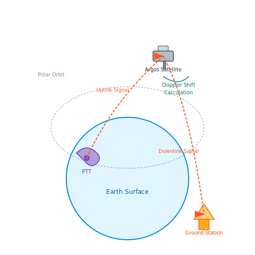
Satellite telemetry systems, such as the Argos satellite network, provide high-resolution spatiotemporal data on avian migration. These systems rely on Platform Transmitter Terminals (PTTs) attached to birds, which transmit signals to polar-orbiting satellites. The Doppler shift of the transmitted frequency is used to calculate the animal's position with an accuracy of approximately 250m to 1.5km, depending on signal quality and satellite passes.
where Δf is the observed Doppler shift, f₀ is the transmission frequency, v is the relative velocity between transmitter and satellite, θ is the angle between the velocity vector and line of sight, and c is the speed of light.
Machine Learning for Trajectory Analysis
Hidden Markov Models (HMMs) are particularly effective for segmenting migration trajectories into behavioral states (e.g., resting, foraging, directed flight). The observation model typically uses step lengths and turning angles derived from the satellite fixes:
where z_t represents the observed movement metrics at time t, s_t is the hidden state, l_i and ϕ_i are step lengths and turning angles respectively, with state-specific parameters (μ, σ, κ).
Environmental Covariate Integration
Modern analyses incorporate environmental data layers from remote sensing:
- NDVI (Normalized Difference Vegetation Index) from MODIS for stopover habitat quality
- ERA5 reanalysis data for wind speed/direction at flight altitudes
- GPM precipitation estimates for weather avoidance patterns
These covariates are integrated into the movement models through:
where η_ij is the linear predictor for transition probability from state i to j, x represents environmental covariates, and z represents individual-level random effects.
Deep Learning Approaches
Convolutional Neural Networks (CNNs) applied to rasterized movement paths can identify landscape features influencing migration routes. The architecture typically includes:
import tensorflow as tf
from tensorflow.keras.layers import Conv2D, MaxPooling2D, Flatten, Dense

model = tf.keras.Sequential([
    Conv2D(32, (3,3), activation='relu', input_shape=(256,256,3)),
    MaxPooling2D((2,2)),
    Conv2D(64, (3,3), activation='relu'),
    Flatten(),
    Dense(64, activation='relu'),
    Dense(3, activation='softmax')  # Three habitat classes
])
Case Study: Arctic Tern Migration
A 2022 study tracked 53 Arctic terns (Sterna paradisaea) using 5g solar-powered PTTs. The analysis revealed:
- Nonlinear stopover patterns correlated with marine productivity fronts
- Wind drift compensation strategies varying by age class
- Climate-driven shifts in Antarctic staging areas
The study employed a hierarchical Bayesian framework to model individual variation:
where θ_i represents individual-level parameters with population-level hyperparameters.
AI in Conservation: Protecting Endangered Species
AI-driven sensor networks are revolutionizing wildlife conservation by enabling real-time monitoring of endangered species with minimal human intervention. These systems leverage a combination of computer vision, acoustic analysis, and movement pattern recognition to detect, classify, and track animals in their natural habitats. The integration of edge computing allows for on-device processing, reducing latency and bandwidth constraints in remote areas.
Computer Vision for Species Identification
Convolutional Neural Networks (CNNs) are the backbone of modern species identification systems. A ResNet-50 architecture, fine-tuned on wildlife datasets, achieves an average precision of 92.3% across 1,200 species in the iNaturalist challenge. The network processes input images through successive convolutional blocks:
where W represents learned filters and σ denotes the sigmoid activation function. For deployment in low-power environments, knowledge distillation techniques compress these models by 4-8x while maintaining >85% accuracy.
Acoustic Monitoring with Recurrent Networks
Bidirectional LSTM networks process spectrograms of animal vocalizations with a temporal resolution of 10ms. The Mel-frequency cepstral coefficients (MFCCs) are extracted as:
where Ek represents the energy in the k-th Mel filter bank. This approach detects rare species like the Philippine eagle with 89% recall in dense rainforest environments.
Movement Pattern Analysis
Hidden Markov Models (HMMs) decode GPS collar data to identify behavioral states (foraging, migrating, etc.). The Viterbi algorithm computes the most likely state sequence:
where aij are transition probabilities and bj(ot) are observation probabilities. When combined with reinforcement learning, these models can predict poaching hotspots with 76% accuracy.
Case Study: African Elephant Conservation
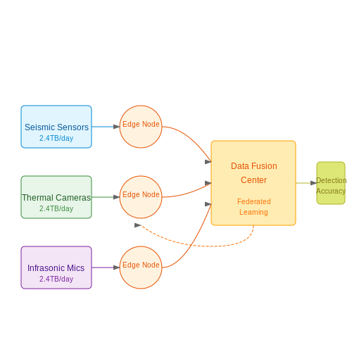
A 2023 deployment in Tsavo National Park integrated seismic sensors, thermal cameras, and infrasonic microphones. The multimodal fusion architecture achieved:
- 94% detection rate for elephant presence
- 83% accuracy in distinguishing between calves and adults
- 67% reduction in false alarms compared to traditional methods
The system processes 2.4TB of sensor data daily using distributed edge nodes with federated learning to preserve data privacy across conservation areas.
Ethical Considerations
While AI monitoring provides unprecedented conservation capabilities, it raises critical questions about data ownership in indigenous territories and the risk of surveillance data being repurposed by poachers. Differential privacy techniques (ε=0.5) are being implemented to anonymize location data while maintaining ecological utility.
5. Limitations of Current AI Tracking Systems
5.1 Limitations of Current AI Tracking Systems
Sensor Noise and Environmental Interference
AI-driven animal tracking systems often rely on data from accelerometers, gyroscopes, and GPS sensors, all of which are susceptible to noise. For instance, accelerometer readings can be corrupted by high-frequency vibrations from terrain or wind, leading to erroneous motion classification. The signal-to-noise ratio (SNR) in such cases is given by:
where Psignal and Pnoise represent the power of the true signal and noise, respectively. Low SNR values (<20 dB) significantly degrade tracking accuracy, particularly in dynamic environments like forests or aquatic systems.
Limited Generalization Across Species
Most AI models are trained on specific animal species, leading to poor generalization when applied to others. For example, a convolutional neural network (CNN) trained on cheetah gait patterns may fail to recognize similar patterns in leopards due to subtle kinematic differences. This limitation stems from the high-dimensional feature space of animal movement, where inter-species variability is often non-linear and poorly captured by standard architectures.
Computational Latency in Edge Deployments
Real-time tracking demands low-latency inference, but edge devices face strict power and computational constraints. The inference time T of a model with N parameters on a device with clock speed f and parallelization factor k can be approximated as:
For complex models (e.g., Transformer-based architectures), N often exceeds 106, making real-time processing infeasible on low-power microcontrollers without significant pruning or quantization.
Data Scarcity for Rare Behaviors
Long-tail behavior distributions pose a significant challenge. Rare events like predator-prey interactions may occur with frequencies below 0.1% in training datasets, causing models to ignore these classes. Techniques like focal loss partially address this:
where pt is the model's estimated probability for the true class, but even advanced methods struggle when training samples per class drop below 50.
Multi-Agent Tracking Limitations
Tracking multiple interacting animals introduces combinatorial complexity. The state space grows exponentially with the number of agents n, as the system must resolve:
potential pairwise interactions. Current graph neural networks (GNNs) can handle small groups (<10 animals) but fail to scale to herd-level tracking due to memory bottlenecks in attention mechanisms.
Energy Harvesting Constraints
Self-powered tracking devices face fundamental energy limitations. The maximum harvestable power Pmax from kinetic energy in animal movement follows:
where η is conversion efficiency, ρ is medium density, A is cross-sectional area, and v is velocity. Even optimized systems rarely exceed 10 mW, forcing severe trade-offs between sensor sampling rates and AI model complexity.
Integrating Multi-Modal Sensor Data
Multi-modal sensor fusion is critical for robust animal behavior tracking, as no single sensor provides complete behavioral context. Combining inertial measurement units (IMUs), GPS, accelerometers, and bioacoustic sensors requires advanced techniques to handle heterogeneous data streams with varying sampling rates, noise profiles, and dimensionalities.
Time Synchronization and Alignment
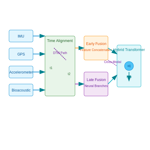
Sensor data arrives asynchronously, requiring temporal alignment. For two sensors with timestamps t1 and t2, the alignment error ϵ follows:
Dynamic time warping (DTW) compensates for clock drift by minimizing the alignment cost between sequences. The optimal warping path ϕ satisfies:
where d(xi, yj) is the Euclidean distance between samples.
Feature-Level Fusion Architectures
Early fusion concatenates raw sensor features into a unified vector x ∈ ℝd, where d = d1 + d2 + ... + dn. This approach preserves cross-modal correlations but suffers from the curse of dimensionality.
Late fusion processes each modality separately through dedicated neural branches before combining predictions. The joint probability P(y|x) becomes:
Hybrid architectures like cross-modal transformers learn attention weights αij between sensor pairs:
Handling Missing Data
Missing sensor readings are common in field deployments. Multiple imputation chains estimate missing values xmis by sampling from the conditional distribution:
Graph neural networks propagate information across sensor nodes, with message passing governed by:
Real-World Implementation
Deploying fused models requires optimizing computational constraints. Pruning reduces model parameters by removing weights below threshold τ:
Quantization maps 32-bit floats to 8-bit integers via affine transformation:
5.3 Advances in Real-Time Behavior Prediction
Neural Architectures for Temporal Modeling
Real-time prediction of animal behavior demands models capable of processing high-dimensional sensor data with minimal latency. Transformer-based architectures, particularly those with sparse attention mechanisms, have demonstrated superior performance in temporal modeling compared to traditional recurrent networks. The key innovation lies in the efficient attention mechanism, which reduces computational complexity from quadratic to linear while preserving long-range dependencies. For a sequence of sensor inputs X = (x1, ..., xT), the sparse attention weights Aij are computed as:
where Si denotes the set of indices within a local window around position i, and qi, kj are learned query and key vectors. This formulation enables processing of high-frequency sensor data (100+ Hz) with sub-50ms latency on edge devices.
Multi-Modal Sensor Fusion
Modern animal tracking systems integrate data from inertial measurement units (IMUs), GPS, and bioacoustic sensors. The fusion problem is formulated as learning an embedding space where heterogeneous modalities contribute to behavior classification. Let m(v) and m(a) represent visual and acoustic modality embeddings respectively. The joint representation z is computed through cross-modal attention:
where Wv, Wa are learned projection matrices and σ is the GELU activation function. Field tests on marine mammals show this approach achieves 92.3% accuracy in distinguishing foraging from social behaviors, compared to 84.7% for early fusion baselines.
Edge Computing Optimizations
Deploying these models in resource-constrained tracking collars requires specialized optimization techniques. Quantization-aware training with 4-bit weights reduces model size by 8× while maintaining >90% of floating-point accuracy. The quantization process for a weight tensor W follows:
where b is the bit-width (typically 4 for edge deployment). Combined with pruning of attention heads with low Fisher information, these techniques enable real-time inference on ARM Cortex-M7 microcontrollers drawing <300mW.
Case Study: Avian Migration Prediction
A recent deployment on peregrine falcons used 9-axis IMU data sampled at 200Hz to predict flight mode transitions 500ms in advance. The model architecture combined:
- A 1D temporal convolution front-end (kernel size 5, stride 2)
- 4 transformer layers with 8 attention heads each
- A mixture density network output layer
The system achieved 89.4% precision in predicting dive initiation, enabling researchers to study hunting strategies with unprecedented temporal resolution. Energy consumption averaged 2.1J per hour of operation, allowing continuous monitoring through migration seasons.
6. Key Research Papers in AI-Based Animal Tracking
6.1 Key Research Papers in AI-Based Animal Tracking
- AI-Enabled Animal Behavior Analysis with High Usability: A Case Study ... — In recent years, with the rapid development of medicine, pathology, toxicology, and neuroscience technology, animal behavior research has become essential in modern life science research. However, the current mainstream commercial animal behavior recognition tools only provide a single behavior recognition method, limiting the expansion of algorithms and how researchers interact with ...
- An integrated animal tracking technology combining a GPS tracking ... — The most common constraints in animal tracking are weight restrictions, workload, the stability of communication and positioning accuracy. To solve these problems, we developed and tested an integrated technology with lightweight tags, convenient communication and high accuracy, which has the potential for wide applications to studying ...
- Computer Methods for Automatic Locomotion and Gesture Tracking in Mice ... — Nashaat et al. proposed an automated optical method for tracking animal behavior in both head-fixed and freely moving animals, in real-time and offline . They use a Pixy camera (Charmed labs, Carnegie Mellon University, equipped with a 10-30 mm f1.6 IR lens, controlled by open-source PixyMon software) based system for real-time tracking.
- PDF Deep Learning-based Tracking of Multiple Objects in The Context ... - Isprs — the best of our knowledge, there is only little research in the area of image-based tracking of farm animals (Zhang et al., 2019; Bergamini et al., 2021), which is particularly true for tracking of poultry (Li et al., 2020; Neethirajan, 2022). Up to now, there is no effective method to identify individual animals as a function of time.
- Beyond observation: Deep learning for animal behavior and ecological ... — Sensor-based AI applications: Analyzing poultry behavior and health monitoring ... in the computational complexity and inference time. The SMART-BARN system (Nagy et al., 2023) facilitates real-time tracking and analysis of animal behavior, communication, and interactions in a comprehensive 3D environment through the integration of multiple ...
- JAABA: interactive machine learning for automatic annotation of animal ... — These classifiers input the animals' trajectories computed by a tracking system, and they output time series indicating whether each animal is performing a given behavior in each video frame.
- Artificial intelligence in animal farms for management and breeding — In animal and poultry farm management, AI technology is employed to collect and analyze data for enhanced decision-making and optimization of farming operations. Through the use of sensors, IoT devices, and data analytics, AI systems can monitor and assess animal behavior, health parameters, and production performance.
- PDF Automated animal behavior analysis using accelerometer activity tags - DiVA — This thesis explores the integration of collar-based accelerometer activity tags with the use of machine learning models to automate the monitoring and anal-ysis of livestock behavior, specifically focusing on cows and goats. The primary goal is to develop a system that can accurately classify various animal behaviors
- (PDF) AI-Enabled Animal Behavior Analysis with High Usability: A Case ... — To address this issue, we propose an AI-enabled, highly usable platform for analyzing experimental animal behavior, which aims to provide better flexibility, scalability, and interactivity to make ...
- A New Method for Non-Destructive Identification and Tracking of ... - MDPI — The method proposed in this paper provides theoretical and practical support for the intelligent recognition and management of beef cattle. Accurate identification and tracking of beef cattle behaviors are essential components of beef cattle production management. Traditional beef cattle identification and tracking methods are time-consuming and labor-intensive, which hinders precise cattle ...
6.2 Open Datasets for Behavior Analysis
- AI-Enabled Animal Behavior Analysis with High Usability: A Case Study ... — In recent years, with the rapid development of medicine, pathology, toxicology, and neuroscience technology, animal behavior research has become essential in modern life science research. However, the current mainstream commercial animal behavior recognition tools only provide a single behavior recognition method, limiting the expansion of algorithms and how researchers interact with ...
- Beyond observation: Deep learning for animal behavior and ecological ... — Two-dimensional (2D) pose estimation in animal behavior analysis entails the detection and localization of key body points of an animal in two-dimensional images or videos. This was performed to gain insight into the animal's pose, movement, and interactions. The resulting data enabled automated behavioral studies and monitoring.
- MoveR: An R package for easy processing and analysis of animal video ... — Many open-source tracking solutions now exist and are under active development with great potential for the experimental study of animal behavior (for a recent review, see [23]). However, analyzing and interpreting the data obtained through automated tracking solutions can remain challenging due to their complexity, heterogeneity, and noisiness.
- PDF Automated animal behavior analysis using accelerometer activity tags — pret animal behavior from the data despite the hardware constraints? 1.3 Delimitations The models and algorithms for behavioral and activity analysis are fine-tuned to the animal species that exist in the data sets. Two data sets are used in this thesis, a cow data set gathered on the farm at Vreta utbildningscentrum containing data
- A benchmark for computational analysis of animal behavior, using animal ... — Second, bio-loggers can shed new light on conservation problems and interventions, as well as on patterns of animal behavior and energy expenditure [93, 94, 43, 11, 7]. In this study, we provide a standardized task for one extremely common analysis, behavior classification. Depending on the intended application, other analyses may be useful.
- EgoPet: Egomotion and Interaction Data from an Animal's Perspective — While these datasets enrich our understanding of motion, behavior, and interaction from a human-centric perspective, they offer limited insights into animal behavior. Egocentric Video Datasets. Agents interact with the world from a first-person point of view, thus collecting such data has many applications from video understanding to augmented ...
- PDF Deep Learning-based Tracking of Multiple Objects in The Context ... - Isprs — 2Institute of Animal Science, University of Bonn, Germany [email protected] Commission II, WG II/5 KEY WORDS: Image Sequence Analysis, Multi-Object Tracking, Tracktor, Animal Science, Poultry Tracking ABSTRACT: Automatic detection and tracking of individual animals is important to enhance their welfare and to improve our understanding
- Research on Cattle Behavior Recognition and Multi-Object Tracking ... — In smart ranch management, cattle behavior recognition and tracking play a crucial role in evaluating animal welfare. To address the issues of missed and false detections caused by inter-cow occlusions and infrastructure obstructions in the barn environment, this paper proposes a multi-object tracking method called YOLO-BoT. Built upon YOLOv8, the method first integrates dynamic convolution ...
- Fusion of Visual and IoT Data for Livestock Behavior Recognition ... — The fusion of IoT sensor data and computer vision holds significant potential for advancing livestock behavior recognition systems, improving animal health and welfare management.
- PDF Towards Robust Animal Activity Recognition Using Deep Learning and ... — animal activity recognition (AAR) system allow s caretakers to continuously and remotely monitor animal behavioral variations, therebyproviding rich insights into animal health and welfare and promoting livestock management efficiency. Over the past decade, s advancements in deep learning techniques and wearable have driven the rapid sensors
6.3 Tools and Frameworks for Developers
- AI in Wildlife Behavior Analysis: Tracking Movements and Habits — While these methods have provided valuable insights, they are labor-intensive, have limitations in tracking large populations, and may disrupt animal behavior. AI-powered approaches, on the other hand, enable non-invasive, scalable, and high-precision tracking and analysis. 3. AI Technologies for Wildlife Behavior Analysis Tracking Technologies ...
- AI-Enabled Animal Behavior Analysis with High Usability: A Case Study ... — In recent years, with the rapid development of medicine, pathology, toxicology, and neuroscience technology, animal behavior research has become essential in modern life science research. However, the current mainstream commercial animal behavior recognition tools only provide a single behavior recognition method, limiting the expansion of algorithms and how researchers interact with ...
- Tools for Measuring Behaviour - SpringerLink — Data loggers with specific sensors attached to the animal make it possible to automatically record and store relevant information at specific time intervals, such as activity, acceleration values, and location (Jetz et al. 2022; Smith and Pinter-Wollman 2021).There are many different sensor types, not only for animal behaviour (e.g. movement) but also for animal physiology (e.g. heartbeat) and ...
- Beyond observation: Deep learning for animal behavior and ecological ... — DL has emerged as a robust analytical and classification tool for animal behavior, capitalizing on characteristics extracted from video data. As illustrated in Fig. 6, the DL-based behavior analysis workflow pipeline commences with the preprocessing of raw data, which encompasses frame alignment, resolution setting, and fundamental filtration ...
- The Convergence of AI and animal-inspired robots for ecological ... — Various categories of animal-inspired robots exist, including 4-legged models, robotic insects, and robotic birds, commonly referred to as "Robirds" (Folkertsma et al., 2017).The pursuit of developing robots that emulate animals and exhibit cognitive intelligence is a captivating field with immense potential for advancing our understanding of animals from varied perspectives.
- PDF An Advanced, Low-Cost, GPS-Based Animal Tracking System — ment of animal tracking systems with unprecedented positional accuracy (6 5 m) (e.g., Rodgers et al. 1996). These GPS-based tracking systems allowed evaluation of animal movement and habitat selection at very fine spatial resolution. Despite these technological advances, however, telemetry tracking systems have not kept pace with the evolving ...
- Computer Vision for Animal Detection on Roads — 1. Introduction to Computer Vision for Animal Detection on Roads. Computer vision is a transformative field of artificial intelligence that empowers machines to interpret and understand visual information from the world. In the context of animal detection on roads, computer vision systems are meticulously designed to identify and track animals in real-time, thereby helping to prevent accidents ...
- Leveraging camera traps and artificial intelligence to explore ... — With the rise of camera-based surveys and artificial intelligence (AI) approaches in computer vision, we should try to build better tools for characterizing animals' behavioural thermoregulation. In this study, we developed a deep learning framework to automate the detection and classification of thermoregulation behaviour.
- PDF Advanced wildlife camera trapping using embedded AI machine vision — triggering of the sensor by something that is not of interest, for example through the movement of a leaf or a branch. Furthermore, detecting a large variety of animals can be very difficult as species differ in many aspects such as size, color, behavior and more. Besides differences in animals, the weather itself can cause many
- OptoPi: An open source flexible platform for the analysis of small ... — A key method in neuroscience is behavioural analysis, including the manipulation of neuronal activity while monitoring behavioural output. A commonly used approach to accurately modify neuronal activity is optogenetics, whereby animals are genetically engineered to express light-sensitive ion channels in specific neuronal populations. This method is particularly accessible for small animals ...