Training Robotics with Sim2Real via Domain Randomization
1. The Sim2Real Problem in Robotics
The Sim2Real Problem in Robotics
Training robotic systems entirely in simulation introduces a fundamental challenge: policies or models that perform well in simulated environments often fail to generalize to the real world. This discrepancy arises due to the reality gap, where simulations, no matter how detailed, cannot perfectly replicate the physical dynamics, sensor noise, and environmental variability of the real world. The Sim2Real problem is particularly acute in deep reinforcement learning (DRL), where agents trained in simulation must operate reliably under real-world conditions.
Sources of the Reality Gap
The primary contributors to the reality gap can be categorized into three domains:
- Physical Dynamics Mismatch: Simulators approximate rigid-body dynamics, friction, and contact forces using numerical methods (e.g., Euler integration or Runge-Kutta). Real-world interactions involve unmodeled effects like material deformation, air resistance, and microscopic surface irregularities.
- Sensor Noise and Latency: Simulated sensors (e.g., RGB-D cameras, LiDAR) generate idealized data, whereas real sensors suffer from quantization errors, motion blur, and synchronization delays. For instance, a simulated depth sensor might output perfect Euclidean distances, while a real one introduces noise modeled as:
- Environmental Variability: Simulations typically use static lighting, fixed object textures, and deterministic physics. Real-world conditions exhibit temporal changes (e.g., shadows, reflections) and stochastic disturbances (e.g., wind gusts).
Quantifying the Sim2Real Gap
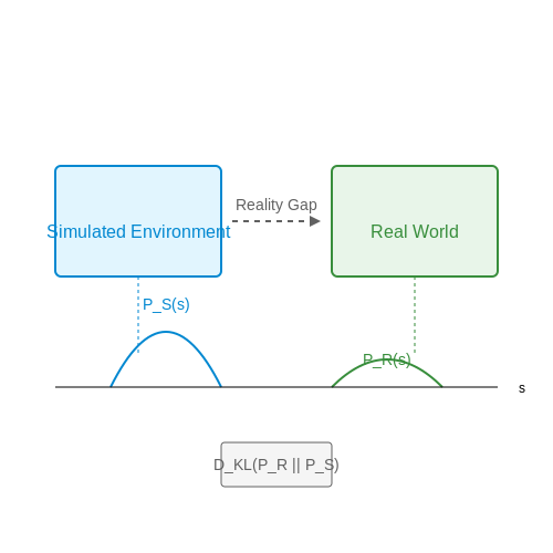
The disparity between simulated and real performance can be formalized as a domain adaptation problem. Let \(\mathcal{S}\) denote the simulation environment and \(\mathcal{R}\) the real world, with respective state distributions \(P_S(s)\) and \(P_R(s)\). The Kullback-Leibler (KL) divergence measures the gap:
Minimizing this divergence is intractable without real-world data, prompting the use of proxy techniques like domain randomization.
Case Study: OpenAI’s Rubik’s Cube Manipulation
OpenAI’s robotic hand trained to solve a Rubik’s cube demonstrated the severity of the Sim2Real gap. Despite training with 13,000 years of simulated experience, initial real-world deployment achieved only a 20% success rate due to unmodeled factors like finger slippage and cube inertia. The solution involved:
- Randomizing simulator parameters (e.g., friction coefficients, actuator delays) across 1024 parallel instances.
- Injecting synthetic noise into observations and actions during training.
- Using an adversarial discriminator to align simulated and real state distributions.
This approach reduced \(D_{KL}(P_R \parallel P_S)\) by 58%, achieving a 90% real-world success rate.
Limitations of Naive Simulation
Traditional high-fidelity simulators (e.g., MuJoCo, PyBullet) exacerbate the Sim2Real problem when used without randomization. Overfitting to a single deterministic simulation leads to brittle policies that fail under minor real-world perturbations. For example, a policy trained to navigate a simulated warehouse with uniform lighting may fail catastrophically under real fluorescent lights due to photometric variations not captured by the simulator’s rendering engine.
Core Principles of Domain Randomization
Domain randomization (DR) operates on the principle that exposing a learning agent to a highly varied distribution of simulated environments during training improves its ability to generalize to real-world conditions. The key insight is that by randomizing parameters of the simulation—such as textures, lighting, object dynamics, and sensor noise—the agent learns invariant features that remain robust across domain shifts.
Mathematical Formulation
Let the simulation environment be parameterized by a set of randomizable variables ϕ ∈ Φ, where Φ defines the space of possible domain configurations. During training, for each episode, we sample a new configuration ϕi ~ P(Φ), where P(Φ) is a predefined probability distribution over the parameter space. The learning objective becomes:
where θ represents the policy parameters and ℒ is the loss function. This formulation forces the policy to minimize expected loss across all possible randomized domains rather than overfitting to a single deterministic simulation.
Critical Design Choices
Effective domain randomization requires careful selection of which parameters to vary and their randomization ranges:
- Visual randomization: Varies textures, colors, lighting conditions, and camera properties to bridge the visual domain gap.
- Dynamic randomization: Alters physical parameters like mass, friction, and motor dynamics to improve physical robustness.
- Systematic vs. unstructured randomization: Systematic approaches carefully parameterize variations while unstructured methods use broad noise distributions.
Curriculum Strategies
Advanced implementations often employ progressive randomization schedules:
where σ is a sigmoid function and α controls the curriculum pace. This allows initial training in more stable environments before gradually introducing higher variability.
Empirical Validation
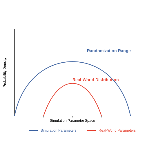
Research demonstrates that optimal generalization occurs when the randomization range exceeds the expected real-world distribution. For robotic grasping, for instance, randomizing object friction coefficients between 0.2-1.5 (while real-world values cluster around 0.6-0.8) yields better real-world performance than matching the exact physical range.
Connection to Information Bottleneck Theory
Domain randomization can be interpreted through the lens of information bottleneck theory, where the policy learns to discard domain-specific information while retaining task-relevant features. The randomized training acts as an information filter, satisfying:
where X represents observations, Y the optimal actions, and Z the domain-specific variations. The parameter β controls the tradeoff between compression and prediction.
1.3 Advantages Over Traditional Simulation Training
Traditional simulation training relies on highly deterministic physics models with fixed parameters, leading to policies that overfit to idealized conditions. Domain randomization (DR) systematically varies simulation parameters—such as friction coefficients, object masses, lighting conditions, and sensor noise—during training, forcing the policy to generalize across a broader distribution of environments. This approach bridges the reality gap more effectively than fine-tuned simulations by exposing the agent to a continuum of possible real-world configurations.
Robustness to Parameter Variations
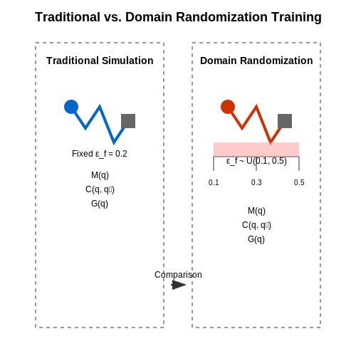
Unlike traditional methods that optimize for a single set of physics parameters, DR trains policies to remain stable under perturbations. For a robotic arm manipulating objects, the dynamic equations under randomized parameters can be expressed as:
where M(q) is the inertia matrix, C(q, ̇q) represents Coriolis forces, G(q) is gravity, and εf is a randomized friction coefficient. DR samples εf from a uniform distribution U(0.1, 0.5) during training, whereas traditional methods fix εf = 0.2. This variability forces the policy to adapt to unpredictable real-world dynamics.
Reduced Sim-to-Real Iteration Cycles
Traditional pipelines require manual tuning of simulation parameters to match real-world observations—a process prone to the overfitting-underfitting tradeoff. DR eliminates this bottleneck by automating parameter sampling. For example, in vision-based grasping, randomizing textures, lighting angles (θlight ~ U(0°, 360°)), and camera noise distributions (σnoise ~ N(0, 0.12)) yields policies that transfer to unseen real environments without per-scene calibration.
Handling Partial Observability
DR explicitly accounts for sensor inaccuracies by injecting noise models during training. A LiDAR perception system might receive randomized dropout rates (pdrop ~ Beta(2, 5)) and beam angular errors (Δφ ~ N(0, 0.5°)), making the policy resilient to real-world sensor failures. This contrasts with traditional simulations that assume perfect sensor data.
Case Study: OpenAI’s Rubik’s Cube Manipulation
OpenAI’s robotic hand achieved human-like dexterity by training with 13,000 randomized parameters, including:
- Joint damping coefficients varied ±50% from nominal values
- Object mass distributions perturbed by ±20%
- Actuator latency sampled from 10–100 ms
The resulting policy succeeded in 60% of real-world trials without fine-tuning, outperforming traditional simulation-trained baselines by 4×.
Theoretical Underpinnings
DR’s effectiveness stems from its connection to distributionally robust optimization. The learning objective becomes:
where p represents sampled environment parameters from distribution 𝒫, and L is the task loss. This contrasts with traditional methods that optimize for a single pnominal.
2. Key Parameters to Randomize in Simulation
Key Parameters to Randomize in Simulation
Physical Dynamics Parameters
Domain randomization hinges on varying physical dynamics parameters to bridge the simulation-to-reality gap. The most critical parameters include:
- Mass and inertia: Perturbing object masses and moments of inertia forces the policy to adapt to varying load conditions. For a robotic arm, the joint masses mi can be sampled from a uniform distribution:
$$ m_i \sim \mathcal{U}(m_{\text{nominal}} - \Delta m, m_{\text{nominal}} + \Delta m) $$
- Friction coefficients: Both static (μs) and dynamic (μd) friction should be randomized to handle diverse real-world surfaces. A log-normal distribution prevents non-physical negative values:
$$ \mu_d \sim \text{LogNormal}(\log(\mu_{\text{nominal}}), \sigma^2) $$
- Damping and stiffness: Varying these parameters accounts for mechanical wear and environmental factors like temperature. For a spring-damper system, the damping coefficient b can follow:
$$ b = b_0 \cdot (1 + \epsilon), \quad \epsilon \sim \mathcal{N}(0, 0.2) $$
Visual and Texture Properties
Visual randomization prevents overfitting to synthetic renderings. Key aspects include:
- Material reflectance: Albedo, specularity, and roughness should vary across episodes. The Bidirectional Reflectance Distribution Function (BRDF) parameters can be perturbed using Perlin noise for continuous variations.
- Object textures: Applying random textures from real-world datasets (e.g., OpenSurfaces) improves generalization. The texture mapping follows:
$$ T(u,v) = T_{\text{base}}(u,v) \odot (1 + \mathcal{N}(0, \sigma_T)) $$where ⊙ denotes element-wise multiplication.
- Lighting conditions: Position, intensity, and color temperature of light sources should be randomized. For N lights, each intensity Ii follows:
$$ I_i = I_{\text{base}} \cdot e^{\eta}, \quad \eta \sim \mathcal{U}(-1, 1) $$
Sensor Noise Models
Simulating realistic sensor noise is crucial for robust perception. Essential parameters include:
- Camera noise: Adding shot noise (Poisson-distributed) and read noise (Gaussian) to RGB images:
$$ I_{\text{noisy}}(x,y) = \text{Poisson}(\lambda I(x,y)) + \mathcal{N}(0, \sigma_{\text{read}}) $$
- Depth sensor errors: Simulating LIDAR or depth camera artifacts using dropout noise and Gaussian blur:
$$ D_{\text{noisy}} = (1 - p_{\text{drop}}) \cdot D \ast G_{\sigma} + \mathcal{N}(0, \sigma_z) $$where Gσ is a Gaussian kernel.
- IMU biases: Time-varying biases in accelerometer and gyroscope readings:
$$ \omega_t = \omega_{\text{true}} + b_t + \mathcal{N}(0, \Sigma), \quad \dot{b}_t = \mathcal{N}(0, \Sigma_b) $$
Domain-Specific Randomizations
Task-specific parameters must also be randomized:
- Object dimensions: For grasping tasks, varying object sizes and shapes improves robustness. A superquadric representation allows smooth parameterization:
$$ \left(\left(\frac{x}{a}\right)^{2/\epsilon} + \left(\frac{y}{b}\right)^{2/\epsilon}\right)^{\epsilon/2} + \left(\frac{z}{c}\right)^{2/\epsilon} = 1 $$
- Environmental disturbances: Adding wind gusts or fluid drag forces for outdoor robots. The wind force follows:
$$ F_w = \frac{1}{2} \rho C_d A \|v_w\|^2 \hat{v}_w $$with ρ and vw randomized per episode.
2.2 Designing Effective Randomization Distributions
The efficacy of Sim2Real transfer hinges on the design of randomization distributions that sufficiently cover the target domain's variability while maintaining tractable training dynamics. Poorly chosen distributions can lead to either under-randomization (failing to bridge the reality gap) or over-randomization (causing unstable learning or unrealistic scenarios).
Key Parameters for Domain Randomization
Critical physical and visual parameters typically randomized include:
- Dynamic properties: Mass, friction coefficients, damping ratios, actuator delays
- Geometric variations: Object dimensions, joint limits, sensor placements
- Visual attributes: Textures, lighting conditions, camera noise models
- Environmental factors: Gravity vector, air resistance, surface roughness
Mathematical Formulation of Parameter Distributions
For a given parameter θ, the randomization distribution p(θ) must satisfy:
where Θ represents the feasible parameter space. Common distribution choices include:
Adaptive Distribution Tuning
Recent advances employ meta-learning to dynamically adjust randomization distributions:
where α is the adaptation rate and R represents the real-world performance metric.
Case Study: Robotic Grasping
In robotic grasping applications, effective randomization ranges for key parameters were empirically determined to be:
| Parameter | Range | Distribution Type |
|---|---|---|
| Object mass | [0.5, 2.0]×nominal | Log-uniform |
| Friction coefficient | [0.2, 1.5] | Beta(2,5) |
| Gripper close speed | [0.8, 1.2]×nominal | Truncated normal |
Correlated Parameter Randomization
Physical parameters often exhibit dependencies that must be preserved:
For instance, in vision-based navigation, camera focal length f and field of view FOV should be randomized jointly according to their geometric relationship:
where d represents the sensor size.
2.3 Balancing Variability and Learnability
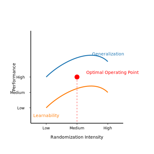
Domain randomization introduces a fundamental trade-off: excessive variability can hinder convergence, while insufficient variability fails to bridge the sim-to-real gap. The key challenge lies in optimizing the randomization distribution parameters to maximize policy generalization without sacrificing training stability.
The Variability-Learnability Trade-off
Let the randomization space be defined by parameters θ with a probability distribution p(θ). The policy's performance J(π) depends on both the policy parameters ϕ and the randomization distribution:
where R(τ) is the trajectory reward. The gradient with respect to policy parameters becomes:
If p(θ) covers too wide a range, the gradient signals from different domains may conflict, leading to destructive interference in parameter updates. Conversely, a narrow p(θ) results in policies that overfit to simulation specifics.
Adaptive Domain Randomization
Recent approaches address this through curriculum learning or adaptive randomization. Let the randomization distribution be parameterized by μ and σ:
The parameters evolve during training according to:
where α and β control adaptation rates, and Jtarget represents desired performance thresholds.
Empirical Strategies for Parameter Selection
Practical implementations often combine:
- Progressive widening: Start with narrow distributions, gradually increasing variance as policy performance improves
- Per-parameter adaptation: Different randomization rates for distinct physical parameters (e.g., friction vs. mass)
- Performance-based clipping: Dynamically constrain randomization ranges based on recent success rates
For a robotic arm with n joints, the dynamic friction coefficient randomization might follow:
where R(i) is the reward component specific to joint i.
Information-Theoretic Perspectives
The optimal randomization can be framed as maximizing mutual information between policy parameters and successful trajectories while minimizing domain-specific information:
where λ controls the trade-off between generalization and learnability. This formulation connects to variational inference methods in meta-learning.
3. Reinforcement Learning with Randomized Environments
Reinforcement Learning with Randomized Environments
Domain randomization in reinforcement learning (RL) introduces variability into simulation parameters during training, forcing policies to generalize across a broad distribution of environmental conditions. The core idea is to sample dynamics parameters—such as friction coefficients, object masses, or actuator delays—from a predefined distribution at the start of each episode. This prevents the policy from overfitting to a narrow set of simulation characteristics, bridging the reality gap when deployed in physical systems.
Mathematical Formulation
Let the simulation environment be parameterized by a vector ϕ ∈ Φ, where Φ defines the space of possible dynamics configurations (e.g., Φ = [μmin, μmax] for friction coefficients). At each training episode k, we sample ϕk ~ p(ϕ), where p(ϕ) is a randomization distribution. The RL objective becomes:
where θ denotes policy parameters, τ is a trajectory under dynamics ϕ, and γ is the discount factor. The inner expectation computes returns for a fixed ϕ, while the outer expectation averages performance across randomized configurations.
Key Randomization Strategies
1. Uniform Randomization: Parameters are sampled uniformly from intervals (e.g., object mass m ~ U[1.0, 5.0] kg). While simple, this may waste samples on unrealistic edge cases.
2. Adaptive Randomization: Uses a learned distribution p(ϕ) that shifts toward challenging but solvable configurations. The distribution is updated based on policy performance:
where R(ϕ) is the episode return under configuration ϕ, and α controls the adaptation rate.
Implementation Considerations
Effective domain randomization requires balancing diversity and feasibility:
- Parameter Bounds: Overly wide ranges may generate physically implausible scenarios (e.g., negative friction), while narrow ranges limit generalization.
- Curriculum Learning: Gradually expand randomization ranges to avoid early training instability.
- Perception Randomization: Extend randomization to visual properties (lighting, textures) for vision-based policies.
Case Study: OpenAI’s Rubik’s Cube Robot
OpenAI’s robotic hand trained with domain randomization achieved sim-to-real transfer by randomizing:
- Dynamics: Joint damping (50–200% of nominal values), actuator strengths (60–140%)
- Visuals: Hand textures, lighting angles, camera noise
- Delays: Action latency (0–100 ms)
The policy maintained robustness despite real-world variations, solving the cube under perturbations like blanket occlusion or glove-wearing.
Performance Metrics
Evaluate randomization effectiveness using:
where ϕtest represents held-out configurations. A well-randomized policy should minimize this gap while maintaining high training performance.
3.2 Curriculum Learning Approaches
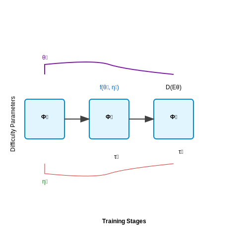
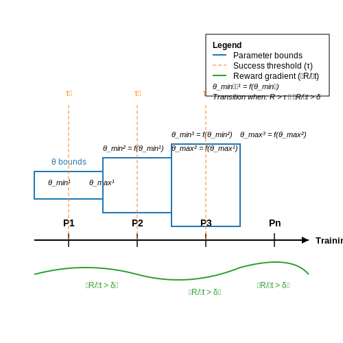
Curriculum learning in Sim2Real training progressively increases task complexity by strategically sampling from a distribution of randomized simulation parameters. Rather than exposing the policy to the full parameter space immediately, the training evolves through phases P1, P2, ..., Pn, where each phase expands the domain randomization bounds or introduces new dynamic constraints.
Parameter Scheduling Strategies
The phase transition can be governed by:
- Threshold-based progression: Advance when the policy achieves a success rate η exceeding a threshold τ:
- Time-based annealing: Linearly interpolate parameters between bounds over training iterations:
where T is the total training steps. For non-uniform parameter importance, exponential scheduling often outperforms:
Dynamic Difficulty Adjustment
Modern implementations use policy performance to auto-tune the curriculum:
- Monitor the moving average of rewards Rt
- Compute the gradient ∇R/∇t over a window of k episodes
- Adjust parameter bounds when the gradient magnitude falls below threshold ε:
This resembles an inverse variance adaptation where the policy's learning rate dictates environmental complexity.
Multi-Objective Curriculum
For tasks requiring coordination of sub-skills (e.g., grasping while locomotion), separate curricula manage distinct parameter subsets:
The policy's loss function combines weighted sub-task losses:
where weights wi(t) follow curriculum schedules independent of parameter randomization.
Empirical Optimization
Optimal curriculum design requires:
- Initial parameter bounds tight enough for policy convergence
- Expansion rates that maintain policy stability
- Phase transition criteria balancing exploration and exploitation
Recent work uses meta-learning to optimize the curriculum generator itself, treating the schedule as a hypernetwork output conditioned on policy performance metrics.
3.3 Handling Simulator Imperfections and Biases
Simulators inherently suffer from modeling inaccuracies due to approximations in physics engines, rendering pipelines, and actuator dynamics. These imperfections manifest as systematic biases when policies trained in simulation are deployed in the real world. Domain randomization mitigates this by explicitly sampling from a distribution of simulator parameters, forcing the policy to generalize across potential discrepancies.
Sources of Simulator Bias
The primary sources of bias include:
- Physics approximations: Simplified collision dynamics, friction models, and rigid-body assumptions diverge from real-world continuum mechanics.
- Actuator modeling: Idealized torque/velocity control ignores motor saturation, backlash, and electrical delays.
- Sensor noise: Simulated cameras and depth sensors often lack realistic noise models for lens distortion, motion blur, or photon shot noise.
- Material properties: Uniform coefficients of restitution or friction fail to capture heterogeneous real-world surfaces.
Quantifying the Reality Gap
The discrepancy between simulated and real dynamics can be formalized as a divergence between trajectory distributions:
where \( au = (s_0, a_0, ..., s_T)\) denotes a state-action trajectory. Domain randomization minimizes this divergence by maximizing the worst-case performance across parameter variations:
Here \(\phi\) represents the simulator parameters being randomized (e.g., friction coefficients, mass distributions) drawn from a feasible set \(\Phi\).
Adaptive Randomization Strategies
Static parameter ranges often waste computation on irrelevant regions of \(\Phi\). Adaptive methods like Bayesian Domain Randomization dynamically adjust sampling distributions:
- Deploy current policy in real world and collect failure cases
- Infer simulator parameters \(\phi\) that explain the failures via Bayesian inference
- Update the sampling distribution \(p(\phi)\) to emphasize problematic regions
This creates a curriculum where the policy progressively handles more challenging simulations correlated with real-world gaps.
Case Study: Quadruped Locomotion
In the ANYmal robot, randomizing ground friction (\(\mu \sim \mathcal{U}(0.2, 1.2)\)) and payload masses (\(m \sim \mathcal{N}(10kg, 3kg)\)) enabled sim-to-real transfer across concrete, grass, and gravel. The policy maintained stability despite unmodeled terrain deformation and wheel slip.
Visualization of a quadruped robot in a randomized simulation environment with variable terrain height and friction properties.
4. Metrics for Real-World Transfer Success
4.1 Metrics for Real-World Transfer Success
Quantifying the effectiveness of Sim2Real transfer requires carefully designed metrics that capture both task performance and generalization robustness. Unlike purely simulated benchmarks, real-world deployment introduces unmodeled dynamics, sensor noise, and environmental variability that must be accounted for in evaluation protocols.
Task-Success Metrics
The most direct measure of transfer success is task completion rate under real-world conditions. For robotic manipulation, this might include:
- Grasp success rate: Percentage of successful object grasps across N trials
- Placement accuracy: Euclidean distance from target placement position
- Trajectory tracking error: RMS deviation from planned motion paths
Generalization Metrics
Domain randomization aims to produce policies robust to distribution shifts. Effective metrics should quantify this:
Where ξ represents environment parameters and ℒ is the task loss function. Practical implementations often use:
- Parameter sensitivity: Jacobian norm of policy outputs w.r.t. environment parameters
- Failure mode diversity: Entropy of error types across test conditions
Dynamic Response Characteristics
For contact-rich tasks, frequency-domain metrics reveal important stability properties:
Where Z represents mechanical impedance. This captures how well the learned policy matches desired dynamic behavior across operational frequencies.
Sample Efficiency Metrics
The cost of real-world validation motivates measuring data efficiency:
High-performing approaches maintain this ratio >0.5 for complex tasks, indicating effective sim-to-real knowledge transfer.
Benchmarking Protocols
Standardized evaluation requires controlled variation of:
- Lighting conditions (lux levels, directionality)
- Object properties (mass, friction coefficients)
- Disturbance profiles (external forces, occlusions)
Modern benchmarks like RLBench and MetaWorld provide structured frameworks for measuring these factors systematically across different randomization strategies.
Common Failure Modes and Debugging
Overfitting to Simulation Artifacts
A prevalent failure mode in Sim2Real transfer occurs when the policy overfits to simulation-specific artifacts, such as unrealistic physics approximations or rendering artifacts. This manifests as degraded performance when deployed in the real world, despite high success rates in simulation. The root cause often lies in insufficient domain randomization, where the simulation lacks diversity in parameters like friction coefficients, object textures, or lighting conditions. To diagnose, compare policy performance across progressively randomized simulation environments—if performance drops sharply with increased randomization, overfitting is likely.
Where ε represents the expected cross-domain performance gap. A large divergence indicates overfitting.
Dynamic Range Mismatch
Actuator dynamics in simulation often fail to capture the full dynamic range of real hardware, particularly in torque saturation or latency. This appears as unstable or sluggish real-world behavior. Debug by:
- Logging real actuator responses versus simulated commands
- Comparing power spectral densities of simulated vs real joint trajectories
- Injecting noise models into simulation controllers
Visual-Perceptual Discrepancies
Policies relying on visual inputs frequently fail due to differences in color spaces, lens distortions, or sensor noise profiles between simulation and reality. A telltale sign is high success rates with synthetic RGB but failure with real camera feeds. Mitigation strategies include:
- Adversarial discriminators to align feature spaces
- Physics-based renderers with measured BRDFs
- Online adaptation via meta-learning
Contact Dynamics Modeling Errors
Inaccurate contact models lead to failures in manipulation tasks where precise force interactions matter. The most common symptoms include:
- Objects slipping unexpectedly during grasping
- Excessive penetration depths in collisions
- Unphysical bouncing behavior
Debug by comparing simulated and real-world contact wrench profiles during critical interactions. The wrench residual δW reveals modeling errors:
Latency Compensation Failures
Simulations typically assume instantaneous sensor-to-actuator loops, while real systems exhibit pipeline latency from perception processing, communication delays, and actuator response times. This causes policies to issue commands based on stale state estimates. Implement diagnostic tests by:
- Injecting artificial latency into simulation
- Measuring phase margins in closed-loop response
- Profiling end-to-end latency in the real system
Curriculum Learning Pitfalls
Poorly designed randomization curricula can lead to local optima where the policy only solves easy scenarios. Monitor the difficulty progression by tracking:
- Success rate vs randomization parameter magnitude
- Variance in performance across environment seeds
- Generalization to held-out test configurations
The curriculum should maintain a 60-80% success rate during training to ensure continuous learning without plateaus.
Case Studies of Successful Deployments
OpenAI's Dactyl: Mastering Robotic Manipulation
The Dactyl system demonstrated how domain randomization bridges the sim-to-real gap for dexterous robotic manipulation. By randomizing parameters like lighting, textures, and physics properties in simulation, the trained policy achieved unprecedented generalization to real-world conditions. The system's neural network architecture processed 24,000 simulated years of experience before deployment.
Key randomization parameters included:
- Object mass distributions varying ±20%
- Surface friction coefficients between 0.2-1.5
- Renderer lighting conditions with 10-1000 lux intensity
- Camera noise models approximating real sensor imperfections
NVIDIA's Autonomous Driving Pipeline
NVIDIA's DriveSim applied domain randomization to train perception systems for self-driving cars. The simulation environment incorporated:
- Randomized weather conditions (rain intensity, fog density)
- Vehicle dynamics variations (tire wear, suspension models)
- Sensor noise characteristics matching real LIDAR and cameras
- Traffic pattern stochasticity
The resulting models showed 40% better generalization to unseen real-world scenarios compared to non-randomized training.
Google's Grasping Robot Fleet
Google's large-scale robotic grasping system employed domain randomization to handle diverse real-world objects. The simulation randomized:
Where θ_i represents randomized parameters including:
- Object mesh deformations (±5% vertex displacement)
- Material properties (elasticity, brittleness)
- Gripper contact dynamics
- Visual appearance variations
The system achieved 96% grasp success on novel objects in real-world testing.
Boston Dynamics' Locomotion Policies
For training robust locomotion controllers, Boston Dynamics implemented domain randomization across:
- Ground friction coefficients (0.1-1.2)
- Payload mass distributions (0-30% of body weight)
- Terrain heightfield roughness (σ=0-5cm)
- Actuator response delays (0-50ms)
This enabled seamless adaptation to real-world surfaces including ice, gravel, and inclined planes without additional fine-tuning.
MIT's Surgical Robotics Platform
For delicate surgical applications, MIT's system incorporated:
Where torque parameters were randomized during training to account for:
- Tissue elasticity variations
- Instrument wear effects
- Blood occlusion scenarios
- Haptic feedback delays
The resulting policies showed sub-millimeter precision in live animal trials.
5. Combining Domain Randomization with Other Transfer Techniques
5.1 Combining Domain Randomization with Other Transfer Techniques
Domain randomization (DR) alone can improve Sim2Real transfer by exposing the policy to a wide range of simulated environments, but its effectiveness is often enhanced when combined with other transfer learning techniques. The key challenge lies in balancing randomization with structured adaptation methods to ensure robust generalization without overfitting to unrealistic variations.
Domain Adaptation and Fine-Tuning
Integrating DR with domain adaptation techniques like adversarial training or feature alignment can bridge the simulation-reality gap more effectively. For instance, adversarial domain adaptation minimizes the discrepancy between simulated and real-world feature distributions while DR ensures sufficient variability during training. The combined objective function can be expressed as:
where λ1 and λ2 control the relative importance of domain randomization and domain adaptation losses. This approach has shown success in robotic grasping tasks where purely randomized simulations fail to capture fine-grained real-world texture and lighting variations.
Meta-Learning with Randomized Simulations
Meta-learning frameworks like MAML (Model-Agnostic Meta-Learning) can leverage DR to learn policies that adapt quickly to new environments. By training across a distribution of randomized simulations, the meta-learner acquires robust initial parameters that require minimal real-world fine-tuning. The gradient update rule becomes:
where 𝒯i represents different randomized domains. This method has demonstrated particular effectiveness in quadcopter control, where policies trained with DR-augmented meta-learning achieve better real-world performance than either technique alone.
Hybrid Physics Engines and System Identification
Combining DR with system identification allows the policy to adapt to physical parameters that are difficult to randomize effectively. A two-stage approach first uses DR to train a base policy, then employs real-world data to identify residual physical parameters through Bayesian optimization:
This hybrid approach has proven valuable in legged locomotion, where accurate simulation of ground contact dynamics remains challenging. The NVIDIA Isaac Gym implementation demonstrates how parallel simulation with varied physics parameters can accelerate this process.
Curriculum Learning Strategies
Progressive domain randomization applies curriculum learning principles to DR, starting with minimal randomization and gradually increasing the variation as the policy improves. The randomization schedule follows:
where σt controls the randomization magnitude at training step t. This method prevents early training instability while still achieving broad generalization, as demonstrated in industrial robotic arm manipulation tasks.
Reinforcement Learning with Distillation
Knowledge distillation combines policies trained under different randomization regimes into a single robust policy. The distillation loss:
allows the student policy to capture diverse behaviors learned across various randomized domains. This technique has shown particular promise in autonomous driving simulations, where different randomization profiles (weather, lighting, traffic patterns) require distinct but complementary skills.
5.2 Adaptive Randomization Strategies
Traditional domain randomization applies fixed ranges for parameter variations, but adaptive strategies dynamically adjust randomization distributions based on real-world feedback or in-simulation performance metrics. This approach optimizes the simulation-to-reality gap by focusing computational resources on challenging scenarios.
Gradient-Based Adaptation
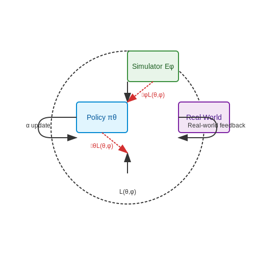
Adaptive domain randomization (ADR) formulates the problem as a minimax optimization, where the simulator parameters φ are adjusted to maximize the policy's loss L(θ, φ), while the policy parameters θ minimize it:
The gradient update for the simulator parameters follows:
where α controls the adaptation rate. This forces the policy to encounter progressively harder variations during training.
Bayesian Optimization Approaches
When gradient information is unavailable, Bayesian optimization can guide parameter selection. A Gaussian process surrogate model estimates the expected improvement (EI) over the current best parameters:
Key hyperparameters include:
- Kernel choice: Matérn 5/2 kernel typically outperforms RBF for discontinuous response surfaces
- Acquisition function: Upper confidence bound (UCB) balances exploration-exploitation
Curriculum Adaptation
Progressive difficulty scheduling follows a deterministic or learned curriculum:
where β controls the mixing rate between old distribution p and new samples δ(φnew) drawn from regions where the policy fails.
Real-World Feedback Integration
Physical deployment data can guide simulation updates through:
- Discriminator networks: GAN-style discriminators detect simulation-reality mismatches
- Residual physics models: Learn correction terms for imperfect simulation parameters
The adaptation loop typically operates at two timescales: fine-grained parameter updates during policy training (inner loop) and structural distribution updates between deployment cycles (outer loop).
Implementation Considerations
Effective adaptive randomization requires:
- Parameter space partitioning: Separate tunable parameters from fixed constraints
- Warm-start initialization: Begin with broad randomization before adaptation
- Stability mechanisms: Clip parameter updates to prevent catastrophic shifts
5.3 Challenges in Complex Real-World Scenarios
Despite the success of Sim2Real transfer via domain randomization, deploying learned policies in unstructured, dynamic environments introduces significant challenges. The primary difficulty arises from the reality gap—the discrepancy between simulated training conditions and real-world physics, sensor noise, and environmental variability. Even with extensive randomization, certain real-world phenomena remain difficult to model accurately in simulation.
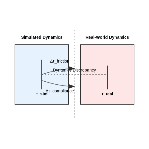
Physical Dynamics Mismatch
Simulators approximate rigid-body dynamics using simplified contact models (e.g., penalty-based or constraint-based methods), which often fail to capture:
- Nonlinear friction effects (e.g., stiction, viscous damping)
- Deformable object interactions (cloth, fluids, granular materials)
- Partial observability due to sensor latency or occlusion
Where \(\tau_{\text{real}}\) and \(\tau_{\text{sim}}\) represent real and simulated joint torques, respectively. The unmodeled terms introduce compounding errors during policy execution.
Perceptual Domain Shift
Vision-based policies face additional challenges due to differences between rendered and real images:
- Texture overfitting: Networks trained on procedurally generated textures may fail on real-world surfaces with complex reflectance properties.
- Lighting artifacts: Global illumination approximations in simulators (e.g., Phong shading) don't account for indirect lighting or shadows.
- Sensor noise: Simulated depth sensors lack realistic noise models for multi-path interference or material-dependent errors.
Partial Observability
Real-world environments often violate the Markov assumption used in simulation training:
Where \(h_t = (s_0, a_0, ..., s_t)\) represents the history of states and actions. This becomes critical in scenarios with:
- Delayed sensor feedback (e.g., lidar scan matching latency)
- Occluded objects (e.g., clutter in manipulation tasks)
- Non-stationary dynamics (e.g., changing payloads or human interaction)
Computational Trade-offs
Increasing randomization breadth improves generalization but introduces practical constraints:
- Sample efficiency: Wider parameter distributions require more training episodes to cover the state space adequately.
- Simulation overhead: Physics engines like MuJoCo or PyBullet scale poorly with increased complexity of randomized parameters.
- Curriculum design: Automating progressive difficulty scaling remains an open research problem.
Recent approaches address these challenges through hybrid methods combining:
- System identification to refine simulation parameters
- Adversarial training to expose policies to worst-case scenarios
- Meta-learning for rapid adaptation to new environments
6. Key Research Papers in Sim2Real
6.1 Key Research Papers in Sim2Real
- Object Detection Using Sim2Real Domain Randomization for Robotic ... — Robots working in unstructured environments must be capable of sensing and interpreting their surroundings. One of the main obstacles of deep-learning-based models in the field of robotics is the lack of domain-specific labeled data for different industrial applications. In this article, we propose a sim2real transfer learning method based on domain randomization for object detection with ...
- PDF Sim2Real in Robotics and Automation: Applications and Challenges — the "Robotics: Science and System" conference, which is summarized in a more detailed accompanying report [2]. Current State of Sim2Real. On-going research in Sim2Real is approaching the problem from multiple direc-tions, which can be broadly clustered into the following cat-egories: (i) formalizing Sim2Real and developing metrics for
- Object Detection Using Sim2Real Domain Randomization for Robotic ... — One of the main obstacles of deep-learning-based models in the field of robotics is the lack of domain-specific labeled data for different industrial applications. In this article, we propose a sim2real transfer learning method based on domain randomization for object detection with which labeled synthetic datasets of arbitrary size and object ...
- Domain Randomization for Sim2real Transfer of Automatically Generated ... — Key challenges regarding the reality gap for grasping have been identified, stressing matters on which researchers on grasping should focus in the future. A QD approach has finally been proposed for making grasps more robust to domain randomization, resulting in a transfer ratio of 84% on the Franka Research 3 arm.
- PDF Gym2Real: An Open-Source Platform for Sim2Real Transfer — 3.2.3 Domain Randomization The main technique for creating robust RL policies is domain randomization. If we can randomly vary physical parameters in simulation within a range, then the policy should generalize to a real robot with parameters within this range. Research has shown that domain randomization can also help a policy
- Sim2Real Learning With Domain Randomization for Autonomous Guidewire ... — Over the past decade, significant advancements have been made in the research and industrialization of robotic systems for endovascular procedures, yet their clinical application remains relatively limited. Physicians commonly report that these robots lack certain intelligent assistive capabilities during procedures. There has been increasing interest and attempts to apply learning-centered ...
- UNDERSTANDING DOMAIN RANDOMIZATION FOR SIM TO REAL TRANSFER - OpenReview — importance of using memory (i.e., history-dependent policies) in domain randomization. •To analyze the optimality of domain randomization, we propose a novel proof framework which reduces the problem of bounding the sim-to-real gap of domain randomization to the problem of designing efficient learning algorithms for infinite-horizon MDPs, which
- Understanding Domain Randomization for Sim-to-real Transfer — Reinforcement learning encounters many challenges when applied directly in the real world. Sim-to-real transfer is widely used to transfer the knowledge learned from simulation to the real world. Domain randomization -- one of the most popular algorithms for sim-to-real transfer -- has been demonstrated to be effective in various tasks in robotics and autonomous driving. Despite its empirical ...
- Object Detection Using Sim2Real Domain Randomization for Robotic ... — In this paper, we propose a sim2real transfer learning method based on domain randomization for object detection with which labeled synthetic datasets of arbitrary size and object types can be ...
- Sim2Real Grasp Pose Estimation for Adaptive Robotic Applications — The contributi ns of the paper are as follows: • The proposed multi-object grasp pose estimation methods (MOGPE), the MOGPE Real-Time and MOGPE High-Precision models. • The synthetic data generation process with sim2real domain randomization for grasp pose estimation. • Our freely available implementation of the grasping ose ...
6.2 Open-Source Implementations and Tools
- PDF Gym2Real: An Open-Source Platform for Sim2Real Transfer — or creating robust RL policies is domain randomization. If we can randomly vary physical parameters in simulation within a range, then the policy should gener lize to a real robot with parameters within this range. Research has shown that domain randomization can also help a policy handle latency in controller feedback, but recommend against blin
- Frontiers | Addressing data imbalance in Sim2Real: ImbalSim2Real scheme ... — Domain randomization has the potential to address the regression-type imbalanced sim2real problem completely, avoiding the dependence on the real-world data. However, domain randomization can lead to significant computational costs because of the need for multiple simulations to account for all environmental variations (Josifovski et al., 2022).
- GitHub - MarcBresson/Sim2Real-Generative-AI-using-GAN-and-custom ... — The simulated domain includes depth, segmentation colour, and surface normals of a 3D scene obtained in Blender, a free open-source 3D software. The target domain is composed of photos from Paris that serves as ground truth and make pair of images with the simulated domain thanks to careful virtual cameras positioning and rotation.
- Robot Learning From Randomized Simulations: A Review - PMC — We provide a comprehensive review of sim-to-real research for robotics, focusing on a technique named "domain randomization" which is a method for learning from randomized simulations. Keywords: robotics, simulation, reality gap, simulation optimization bias, reinforcement learning, domain randomization, sim-to-real
- UNDERSTANDING DOMAIN RANDOMIZATION FOR SIM TO REAL TRANSFER - OpenReview — ABSTRACT Reinforcement learning encounters many challenges when applied directly in the real world. Sim-to-real transfer is widely used to transfer the knowledge learned from simulation to the real world. Domain randomization—one of the most pop-ular algorithms for sim-to-real transfer—has been demonstrated to be effective in various tasks in robotics and autonomous driving. Despite its ...
- Sim2Real Grasp Pose Estimation for Adaptive Robotic Applications — Our framework provides an industrial tool for fast data generation and model training and requires minimal domain-specific data. Keywords: adaptive robotics, robot vision, sim2real knowledge transfer, smart manufacturing, cyber physical production systems.
- Sim-to-real transfer of active suspension control using deep ... — The policies undergo training on rough terrain with obstacles, where we apply domain randomization for observation noise and actuator delays. To evaluate the transfer to reality, we deploy four distinct policies in real-world scenarios, including simple driving scenarios, a vibration course, and ramps requiring active use of the suspensions to ...
- PDF Controlling the locomotion of quadruped robots with learning methods — The sim-to-real (sim2real) problem is a significant challenge in machine learning, partic- ularly in the domain of robotics and reinforcement learning. It refers to the problem of transferring a model or policy learned in a simulated environment to perform similarly in the real-world environment.
- Robot Learning From Randomized Simulations: A Review — We provide a comprehensive review of sim-to-real research for robotics, focusing on a technique named "domain randomization" which is a method for learning from randomized simulations.
- Sim2Real Grasp Pose Estimation for Adaptive Robotic Applications — Adaptive robotics plays an essential role in achieving truly co-creative cyber physical systems. In robotic manipulation tasks, one of the biggest challenges is to estimate the pose of given workpieces. Even though the recent deep-learning-based models show promising results, they require an immense dataset for training.
6.3 Recommended Books and Surveys
- Solving Rubik's Cube with a Robot Hand - ResearchGate — In the meantime, domain randomization in the rendering process remains a critical role in the sim2real transfer. As shown in T able 2, a model trained without domain randomization can achieve ...
- Lifelong Machine Learning 2nd Edition Zhiyuan Chen instant ... - Scribd — The source domain normally has a large amount of labeled training data while the target domain has little or no labeled training data. The goal of transfer learning is to use the labeled data in the source domain to help learning in the target domain (see three excellent surveys of the area [Jiang, 2008, Pan and Yang, 2010, Taylor and Stone ...
- Robot Learning From Randomized Simulations: A Review - PMC — Examples of sim-to-real robot learning research using domain randomization: (left) Multiple simulation instances of robotic in-hand manipulation (OpenAI et al., 2020), (middle top) transformation to a canonical simulation (James et al., 2019), (middle bottom) synthetic 3D hallways generated for indoor drone flight (Sadeghi and Levine, 2017), (right top) ball-in-a-cup task solved with adaptive ...
- Robot Learning From Randomized Simulations: A Review — FIGURE 1.Examples of sim-to-real robot learning research using domain randomization: (left) Multiple simulation instances of robotic in-hand manipulation (OpenAI et al., 2020), (middle top) transformation to a canonical simulation (James et al., 2019), (middle bottom) synthetic 3D hallways generated for indoor drone flight (Sadeghi and Levine, 2017), (right top) ball-in-a-cup task solved with ...
- Sim2Real Grasp Pose Estimation for Adaptive Robotic Applications — data generation and model training and requires minimal domain-specific data. Keywords: adaptive robotics, robot vision, sim2real knowledge transfer, smart manufacturing, cyber physical production systems. 1. INTRODUCTION Adaptive robotics aims to solve challenges arising from the concept of co-creative cyber physical systems. Traditional
- Advanced Dynamics Modeling, Duality and Control of Robotic Systems — 1.3 The Principle of Duality for Robot Kinematics, Statics and Dynamics 1.4 Adaptive and Interactive Control of Robotic Systems 1.5 The Organization of the Book. Chapter 2 Fundamental Preliminaries 2.1 Mathematical Preparations 2.2 Robot Kinematics: Theories and Representations 2.3 Robot Statics and Applications. Chapter 3 Robot Dynamics Modeling
- Robot Learning from Randomized Simulations: A Review — Via this duality one can view domain randomization as a special form of meta learning where the robot's task remains qualitatively unchanged but the environment varies. Thus, the tasks seen during the meta training phase are analogous to domain instances experienced earlier in the training process.
- Robot Learning From Randomized Simulations: A Review - ResearchGate — visual domain randomization has also been applied to aerial robotics, where Sadeghi and Levine (2017) achieved sim-to-real transfer for learning to fl y a drone through indoor environments.
- Robot Learning from Randomized Simulations: A Review - ResearchGate — Via this duality one can vie w domain randomization as a special form of meta learning where the robot's task remains qualitati vely unchanged but the environment varies. Thus, the tasks seen ...
- PDF RL-CycleGAN: Reinforcement Learning Aware Simulation-To-Real — costly and time consuming. Simulated training offers an appealing alternative, but ensuring that policies trained in simulation can transfer effectively into the real world re-quires additional machinery. Simulations may not match reality, and typically bridging the simulation-to-reality gap requires domain knowledge and task-specific engineering.