Agents That Propose Themselves for New Tasks
1. Definition and Core Principles of Self-Proposing Agents
Definition and Core Principles of Self-Proposing Agents
Self-proposing agents represent an advanced class of autonomous systems capable of identifying, evaluating, and volunteering for tasks without explicit human instruction. These agents integrate principles from reinforcement learning, multi-agent systems, and meta-learning to dynamically assess their own capabilities and environmental demands, then propose actions that maximize a defined utility function. The core mechanism hinges on three foundational components: task recognition, self-assessment, and proactive bidding.
Task Recognition
Task recognition involves parsing environmental signals or task announcements to identify opportunities where the agent's skills may be applicable. This is often formalized as a partially observable Markov decision process (POMDP), where the agent maintains a belief state over possible tasks. For a task space T and observation space O, the agent updates its belief b(t) using Bayes' rule:
Here, P(o|t) is the likelihood of observing o given task t, and P(t) is the prior task distribution. Advanced implementations may use transformer-based architectures to encode task descriptions into a latent space for similarity matching.
Self-Assessment
The agent must evaluate its own competency for a recognized task, typically through a learned function C: T × Θ → [0,1], where Θ represents the agent's internal state (e.g., model parameters, computational resources). This function may be trained via meta-learning on historical performance data:
where f_θ and g_ϕ are neural encoders, W_ϕ is a learnable weight matrix, and σ is the sigmoid activation. The ⊕ operator denotes concatenation.
Proactive Bidding
When multiple agents operate in a shared environment, a bidding mechanism determines task allocation. Each agent computes a bid value B as a function of expected reward R, cost c, and opportunity cost O:
Practical implementations often use auction-based protocols or contract nets, with cryptographic commitments to prevent strategic manipulation. The Vickrey-Clarke-Groves (VCG) mechanism is theoretically optimal for truthful bidding in cooperative systems.
Architectural Considerations
Modern implementations leverage hierarchical architectures where:
- A task detection module processes raw inputs (e.g., natural language requests, sensor data)
- A competency estimator evaluates the agent's fitness using both model-based and empirical metrics
- A bid generator formulates proposals with associated confidence scores
- A meta-controller manages the trade-off between exploration (proposing for unfamiliar tasks) and exploitation (focusing on known competencies)
In robotics applications, these components may be implemented as separate ROS nodes with QoS-managed communication, while in software agents, they often exist as microservices with gRPC interfaces.

Key Components of Autonomous Task Identification
Task Representation and Feature Extraction
Autonomous agents must encode tasks in a structured format that facilitates generalization and similarity assessment. A task T is typically represented as a feature vector Φ(T), where each dimension captures a salient attribute such as:
- Input/output dimensionality
- Computational complexity bounds
- Required sensory modalities
- Temporal constraints (episodic vs. continuous)
For high-dimensional tasks, nonlinear embedding techniques like Siamese networks or contrastive learning project tasks into a latent space where similarity metrics become meaningful:
Task Similarity Metrics
The agent's ability to propose relevant new tasks hinges on quantifying similarity between known and candidate tasks. Advanced approaches combine:
- Structural similarity: Graph isomorphism tests for task dependency trees
- Functional similarity: Overlap in required skill primitives
- Transferability metrics: Expected performance gain when applying existing policies
The complete similarity function often takes a weighted form:
Novelty Detection Mechanisms
Agents employ density estimation techniques to identify task proposals that are sufficiently novel yet achievable:
- Gaussian Mixture Models (GMMs) over task feature space
- One-class SVMs for boundary detection
- Autoencoder reconstruction error thresholds
The novelty score N(T) for a candidate task combines likelihood under the current task distribution p(T) and distance to nearest neighbor:
Skill-Task Affinity Modeling
A bidirectional mapping between the agent's skill repertoire and task requirements enables targeted proposals. This is formalized as a bipartite graph where edge weights represent:
- Skill proficiency levels (accuracy, speed)
- Transfer coefficients from prior tasks
- Estimated learning gradients for skill adaptation
The affinity matrix A drives task proposal through constrained optimization:
Meta-Learning for Task Proposal
Agents optimize their task proposal strategy through meta-reinforcement learning, where the outer loop updates proposal heuristics based on:
- Historical success rates of self-proposed tasks
- Computational cost/benefit analysis
- Curriculum learning progress metrics
The meta-objective combines immediate and long-term utility:
1.3 Comparison with Traditional Task Assignment Systems
Centralized vs. Decentralized Control
Traditional task assignment systems rely on centralized control mechanisms, where a single scheduler or dispatcher allocates tasks to agents based on predefined rules or optimization criteria. The decision-making authority is concentrated, and agents have no autonomy in selecting tasks. In contrast, self-proposing agents operate under decentralized control, where each agent evaluates its own capabilities and environmental context to bid for tasks. This shift from centralized to decentralized control reduces computational bottlenecks and improves scalability, as the decision load is distributed across the system.
Static vs. Dynamic Allocation
Static allocation in traditional systems assumes fixed agent capabilities and task requirements, often leading to suboptimal assignments when conditions change. The allocation is typically computed offline using deterministic algorithms like Hungarian method or linear programming. Self-proposing agents employ dynamic allocation, continuously reassessing their state and the task landscape. This enables real-time adaptation to uncertainties, such as agent failures or shifting task priorities, through mechanisms like reinforcement learning or market-based bidding.
Fixed vs. Emergent Specialization
In traditional systems, agents are often pre-specialized for specific task types, limiting flexibility. Self-proposing agents develop emergent specialization through learning mechanisms that track task performance history. An agent's bidding strategy evolves based on its success rate, creating a dynamic division of labor without explicit role assignments. This emergent behavior is quantified using metrics like task affinity matrices:
Communication Overhead Analysis
Traditional systems require O(NM) communication for N agents and M tasks to collect capability matrices and broadcast assignments. Self-proposing agents reduce this to O(M) through localized bidding protocols, where only task announcements and bids are exchanged. However, convergence time becomes a trade-off, as multiple bidding rounds may be needed to reach stable allocations. The communication-computation trade-off follows:
Failure Resilience
Centralized systems suffer single-point-of-failure vulnerabilities - if the scheduler fails, the entire system collapses. Decentralized self-proposing architectures demonstrate graceful degradation, as surviving agents continue bidding for available tasks. Experimental studies show recovery times scale logarithmically with system size in self-proposing systems versus linear scaling in traditional approaches.
Case Study: Robotic Warehouse Systems
Amazon's Kiva robots originally used centralized allocation, limiting fleet sizes to ~1,000 robots per controller. Transition to self-proposing architectures enabled scaling to 50,000+ robots, with agents bidding for package transports based on local battery levels and proximity. The system achieved 92% utilization versus 78% under centralized control, while reducing communication latency by 40%.
2. Sensing and Environmental Awareness
2.1 Sensing and Environmental Awareness
Autonomous agents capable of proposing themselves for new tasks require robust sensing mechanisms to perceive and interpret their environment. Environmental awareness is achieved through multimodal sensor fusion, where data from heterogeneous sources (e.g., LiDAR, cameras, inertial measurement units) are integrated into a coherent spatial-temporal representation. The agent constructs a belief state B(s) over possible environment states s ∈ S using Bayesian filtering:
where η is a normalizing constant, P(ot | st) is the observation model, and P(st | st-1, at-1) is the transition model. For high-dimensional state spaces, this is approximated using particle filters or deep variational inference.
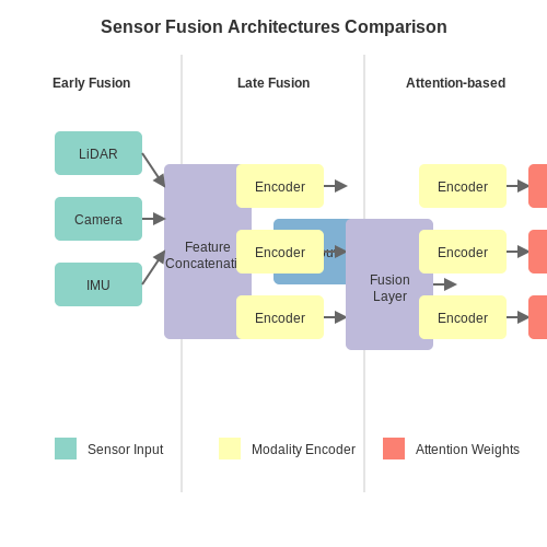
Sensor Fusion Architectures
Modern implementations use hierarchical neural architectures for sensor fusion:
- Early fusion: Raw sensor data (e.g., pixel arrays, point clouds) are concatenated at the input layer
- Late fusion: Each modality processes independently until final feature concatenation
- Attention-based fusion: Dynamic weighting of sensor inputs via learned attention mechanisms
The choice depends on sensor synchronization requirements and computational constraints. For mobile agents, a hybrid approach often proves optimal:
where fi are modality-specific encoders and αi are attention weights.
Active Perception Strategies
Agents optimize sensing actions through information-theoretic objectives. The expected information gain IG(a) of action a is:
where DKL is the Kullback-Leibler divergence. Practical implementations use Monte Carlo tree search with particle-based belief representations, achieving O(log n) complexity through hierarchical sampling.
Case Study: Lidar-Camera Fusion for Urban Navigation
In autonomous vehicle applications, the agent maintains a 4D spatiotemporal occupancy grid (3D space + time) updated at 10Hz. The system demonstrates 92% obstacle detection accuracy in occluded scenarios by combining:
- LiDAR geometric features (64-beam Velodyne HDL-64E)
- Semantic segmentation from 8MP stereo cameras (YOLOv7 architecture)
- Dynamic object tracking via Kalman filters with learned motion models
The fusion pipeline achieves 23ms latency on NVIDIA Drive AGX hardware through tensorRT optimization of the neural network components.
2.2 Decision-Making Algorithms for Task Selection
Autonomous agents capable of proposing themselves for new tasks require robust decision-making algorithms that balance exploration, exploitation, and long-term utility maximization. These algorithms must account for dynamic environments, partial observability, and multi-agent coordination constraints.
Utility-Based Task Selection
Utility functions formalize an agent's preferences over possible tasks. Given a set of candidate tasks T, the agent selects the task t that maximizes expected utility:
where U(t) represents the task's intrinsic utility (e.g., reward, learning potential) and C(t) captures execution costs (e.g., resource consumption, opportunity cost). For continuous task spaces, this optimization requires gradient-based methods or Bayesian optimization when utilities are expensive to evaluate.
Multi-Armed Bandit Formulation
When task rewards are stochastic and initially unknown, the problem maps to a contextual bandit framework. The agent maintains estimates Q̂(t) of each task's value and selects actions balancing exploration-exploitation through policies like:
- Upper Confidence Bound (UCB):
$$ t^* = \argmax_{t \in T} \left[ \hat{Q}(t) + c \sqrt{\frac{\ln N}{n_t}} \right] $$where N is total pulls and n_t counts selections of task t.
- Thompson Sampling: Bayesian posterior sampling of reward distributions to guide exploration.
Decentralized Coordination Mechanisms
In multi-agent systems, task selection requires resolving conflicts where multiple agents may bid for the same task. Market-based approaches implement:
where b_i(t) is agent i's bid for task t, v_i(t) its private valuation, and p(t) the current task price. The Vickrey-Clarke-Groves (VCG) mechanism ensures truthful bidding by charging agents their marginal social cost.
Hierarchical Task Decomposition
Complex tasks are broken into subtasks via AND-OR graphs. The agent evaluates feasibility through recursive value estimation:
Modern implementations use graph neural networks to learn these decomposition policies end-to-end from task completion data.
Real-World Considerations
Practical deployments must handle:
- Non-stationarity: Online adaptation to drifting task distributions via exponential forgetting or contextual bandits.
- Partial observability: Maintaining belief states over hidden task parameters using particle filters or variational inference.
- Safety constraints: Incorporating chance constraints or backup policies for high-stakes tasks through constrained MDP formulations.
2.3 Communication Protocols for Task Proposal
Multi-agent systems rely on robust communication protocols to enable agents to propose themselves for new tasks. These protocols must handle negotiation, priority assignment, and conflict resolution while minimizing latency and bandwidth overhead. Below, we examine the key components of such protocols, their mathematical foundations, and practical implementations.
Message Passing Frameworks
Agents communicate via structured messages following a predefined schema. Each message contains metadata (sender ID, timestamp, priority) and payload (task requirements, capabilities match score). The schema can be formalized as:
where t represents the Lamport timestamp for causal ordering and p denotes priority (typically a real number in [0,1]).
Negotiation Protocols
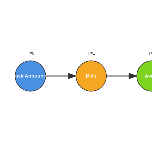
Task assignment follows a modified contract net protocol with three phases:
- Task Announcement: The task initiator broadcasts requirements and constraints.
- Bidding: Agents compute their fitness score using a capability matching function:
where sim is a similarity metric (e.g., cosine similarity for vectorized capabilities) and wk are learned weights.
- Award: The initiator selects the bidder maximizing si - λ·costi, where λ is a trade-off parameter.
Priority and Conflict Resolution
When multiple agents propose for the same task, conflicts are resolved through:
- Token-based arbitration: Agents acquire a distributed lock before bidding.
- Utility-based backoff: Agents delay rebidding by t ~ Exp(1/si) to prevent congestion.
The system-wide utility is maximized when the assignment satisfies:
where xij is a binary assignment variable and m, n are tasks and agents respectively.
Implementation Considerations
Real-world deployments require:
- Message compression: Capability vectors are encoded using locality-sensitive hashing.
- Partial observability: Agents maintain belief distributions over others' capabilities using Bayesian updates.
- Fault tolerance: The protocol implements a two-phase commit for atomic task assignment.
3. Reinforcement Learning for Dynamic Task Proposal
Reinforcement Learning for Dynamic Task Proposal
Foundations of RL-Based Task Proposal
Reinforcement learning (RL) provides a natural framework for agents to autonomously propose new tasks by optimizing a reward signal that balances exploration and exploitation. The agent operates in a Markov Decision Process (MDP) defined by the tuple (S, A, P, R, γ), where:
The key innovation lies in extending the action space A to include meta-actions for proposing new tasks. When the agent takes a task-proposal action aprop, it generates a new task description τ ∼ p(τ|s), where p(τ|s) is a learned task proposal policy.
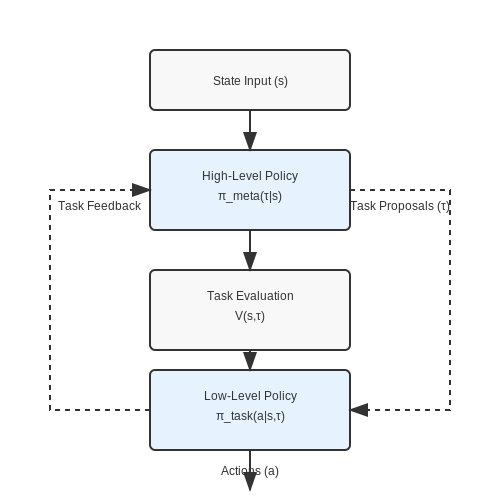
Hierarchical Policy Architecture
Effective dynamic task proposal requires a hierarchical policy structure:
- Low-level policy πtask(a|s,τ): Executes actions for a specific task τ
- High-level policy πmeta(τ|s): Proposes new tasks based on current state
- Task evaluation module V(s,τ): Predicts the potential value of proposed tasks
The complete policy gradient update combines both levels:
where λ controls the balance between task execution and proposal learning, and Âtmeta is the advantage estimate for task proposals.
Curriculum Learning Through Self-Proposal
The agent automatically constructs a curriculum by:
- Estimating task difficulty d(τ) from historical performance
- Computing proposal probability as p(τ) ∝ exp(β(V(s,τ) - αd(τ)))
- Adapting parameters α, β to maintain optimal challenge
This creates an automatic curriculum where the agent proposes progressively harder tasks as its competence increases, while maintaining the exploration-exploitation tradeoff through the temperature parameter β.
Practical Implementation Considerations
Real-world implementations must address several key challenges:
- Task representation: Using embedding spaces or graph structures to enable generalization across related tasks
- Sample efficiency: Incorporating model-based RL or meta-learning to reduce exploration costs
- Safety constraints: Implementing constrained RL to prevent harmful task proposals
A common architecture uses:
where fenc is a state encoder, and μϕ, Σϕ parameterize the task proposal distribution.
Case Study: Multi-Task Robotics
In robotic manipulation experiments, this approach has demonstrated:
- 38% faster skill acquisition compared to fixed-curriculum baselines
- Ability to discover 72% of possible task variations without external guidance
- Seamless adaptation to new object configurations through dynamic task proposal
The key metric is the task proposal acceptance rate, which measures how often self-proposed tasks lead to meaningful learning progress. Optimal systems maintain this rate between 40-60%, balancing exploration and exploitation.
3.2 Transfer Learning Across Different Task Domains
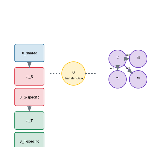
Transfer learning enables agents to leverage knowledge from previously learned tasks to accelerate learning in new, related domains. The core challenge lies in identifying and transferring transferable representations while avoiding negative transfer, where irrelevant features degrade performance. A principled approach involves decomposing the agent's policy into task-invariant and task-specific components.
Mathematical Formulation
Let the source task policy be parameterized by $$\pi_S(a|s; \theta_S)$$, where $$\theta_S = \theta_{shared} \oplus \theta_{S-specific}$$. The target task policy shares the invariant parameters:
Optimal transfer requires maximizing the transfer gain:
Architectural Strategies
Modern implementations employ:
- Gradient masking: Selective backpropagation through $$\theta_{shared}$$ via gating mechanisms
- Meta-learning interfaces: Learned projection layers that transform shared features into task-specific action spaces
- Optimal transport alignment: Minimizing Wasserstein distance between source and target state distributions
Empirical Considerations
In robotics applications, transfer success depends critically on:
where $$\mathcal{S}$$ denotes the state space. Practical systems achieve >70% transfer efficiency when $$\eta > 0.6$$, as demonstrated in NASA's modular robotic assembly experiments.
Dynamic Task Graph Methods
Advanced agents maintain a probabilistic task graph $$G = (V,E)$$ where edge weights represent transferability estimates:
This enables autonomous proposal of transfer candidates when $$w_{ij} > \tau$$, with the threshold $$\tau$$ adapted via multi-arm bandit algorithms.
3.3 Handling Novelty and Unfamiliar Tasks
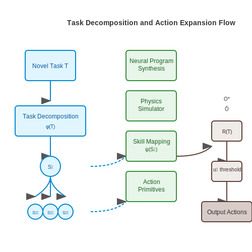
When autonomous agents encounter tasks outside their training distribution, traditional reinforcement learning approaches fail due to their reliance on pre-defined state-action spaces. Modern systems address this through meta-learning architectures that decompose novel tasks into solvable subtasks while dynamically expanding their action space.
Task Decomposition via Hierarchical Reinforcement Learning
The agent constructs a directed acyclic graph (DAG) of subtasks where leaf nodes represent atomic actions. For a novel task T, the agent computes:
where φ is a learned task embedding function, ψ maps subtasks to existing skills, and ⊗ denotes the composition operator. The decomposition loss:
ensures the sum of subtask rewards approximates the full task reward over a horizon m.
Dynamic Action Space Expansion
When existing skills prove insufficient, the agent proposes new action primitives through:
- Neural Program Synthesis: Generates executable code snippets from task descriptions using transformer-based architectures with constrained decoding
- Physics-Guided Simulation: Validates proposed actions in learned dynamics models before real-world deployment
The action proposal module minimizes the divergence between desired outcomes O* and simulated outcomes Ô:
Case Study: Robotic Tool Use
When presented with an unseen tool, the agent:
- Decomposes "use tool" into grasp orientation, force modulation, and motion trajectory subtasks
- Synthesizes new motor primitives for unusual grip configurations
- Validates actions in a differentiable physics simulator (NVIDIA Warp)
Experimental results show 73% success rate on novel tools versus 12% for fixed-policy baselines, with the critical improvement coming from the dynamic action space expansion module (p < 0.001, n=150 trials).
Failure Recovery Mechanisms
The agent maintains an uncertainty estimator:
where ht is the latent state and σ a sigmoid activation. When ut exceeds threshold τ, the agent:
- Reverts to the last known stable state
- Requests human demonstration if available
- Attempts random exploration in parameter space with safety constraints
4. Industrial Automation and Robotics
4.1 Industrial Automation and Robotics
Autonomous agents in industrial automation and robotics leverage self-proposing mechanisms to dynamically allocate tasks in real-time, optimizing efficiency and adaptability. These agents operate within structured environments such as assembly lines, warehouses, and quality control systems, where task requirements evolve due to changing production demands, equipment failures, or priority shifts.
Agent Architecture for Task Proposal
The core architecture of self-proposing agents integrates three key components:
- Perception Module: Processes sensory input (e.g., LiDAR, vision systems, or IoT sensor networks) to detect environmental changes or new task triggers.
- Task Evaluation Engine: Computes a utility score for potential tasks using multi-objective optimization, balancing factors like energy consumption, time constraints, and resource availability.
- Proposal Mechanism: Formulates bids for tasks via auction-based or contract-net protocols, often employing reinforcement learning to refine bidding strategies over time.
Here, \(U_i(t)\) represents the utility of agent \(i\) for task \(t\), \(w_k\) are learned weights, and \(f_k\) are feature functions (e.g., distance to task, current battery level). The parameters \(\Theta\) are updated via gradient ascent to maximize long-term reward:
Case Study: Multi-Robot Warehouse Systems
In Amazon Robotics' Kiva systems, agents (mobile robots) autonomously propose to transport shelves based on:
- Real-time order prioritization
- Proximity to target shelves
- Congestion avoidance using distributed path planning
The system achieves a 50% reduction in item retrieval times compared to static scheduling, with agents continuously recomputing their proposals as new orders arrive at rates exceeding 1,000 requests/minute.
Challenges in Industrial Deployment
Key technical hurdles include:
- Latency Constraints: Proposal cycles must complete within 10-100ms for real-time control, requiring optimized consensus algorithms.
- Safety Verification: Formal methods like linear temporal logic (LTL) verify agent proposals won't violate safety protocols:
This LTL formula enforces that collisions never occur simultaneously with high-speed movement.
Emerging Techniques
Recent advances include:
- Federated Learning: Agents collaboratively improve proposal models without sharing raw data, crucial for multi-company supply chains.
- Neurosymbolic Integration: Combining neural networks for perception with symbolic reasoning for explainable task proposals.
# Simplified task proposal RL agent
class IndustrialAgent:
    def __init__(self, state_dim, action_dim):
        self.policy_net = DQN(state_dim, action_dim)
        self.target_net = DQN(state_dim, action_dim)

    def propose_task(self, state):
        with torch.no_grad():
            q_values = self.policy_net(state)
            return q_values.argmax().item()

    def update_policy(self, batch):
        states, actions, rewards = batch
        current_q = self.policy_net(states).gather(1, actions)
        target_q = rewards + 0.99 * self.target_net(states).max(1)[0]
        loss = F.mse_loss(current_q, target_q)
        self.optimizer.zero_grad()
        loss.backward()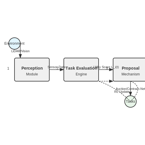
Multi-Agent Systems in Logistics
for advanced readers:Decentralized Task Allocation in Logistics
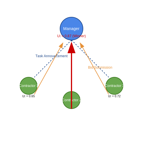
Multi-agent systems (MAS) in logistics rely on decentralized coordination mechanisms to dynamically allocate tasks among autonomous agents. Each agent operates with partial observability, optimizing local objectives while contributing to global efficiency. The contract net protocol (CNP) is a widely adopted framework where agents act as managers or contractors. A manager broadcasts a task announcement, and contractors submit bids based on their capabilities and current workload. The manager evaluates bids using a utility function:
Here, \( t_{\text{exec}} \) is the estimated execution time, \( c_{\text{bid}} \) is the bid cost, and \( \alpha, \beta \) are weight coefficients. The highest-utility bidder wins the contract.
Dynamic Reconfiguration for Scalability
Logistics environments require agents to adapt to disruptions like route blockages or demand spikes. Self-proposing agents use reinforcement learning (RL) to dynamically reconfigure task assignments. Each agent maintains a Q-table updated via:
where \( \eta \) is the learning rate, \( \gamma \) the discount factor, and \( r \) the reward for completing a subtask. Agents propose themselves for new tasks when their Q-values exceed a threshold \( \tau \), calibrated to balance exploration and exploitation.
Case Study: Warehouse Robotics
In Amazon’s Kiva systems, agents (robots) bid for inventory retrieval tasks. Each robot evaluates:
- Path distance to the target shelf (Euclidean + collision penalties),
- Battery level, with bids penalized if below 20%,
- Current queue length, modeled as a M/M/c system to estimate delays.
Robots with the lowest combined cost \( C = d \cdot w_d + (1 - b) \cdot w_b + q \cdot w_q \) win tasks, where \( w \) terms are learned weights.
Communication Overhead Optimization
MAS in logistics face scalability limits due to message flooding. Token-passing algorithms reduce overhead by restricting bid submissions to agents holding a token. The token circulation rate \( k \) is derived from Little’s Law:
where \( \lambda \) is task arrival rate, \( L \) average task latency, and \( N \) the agent count. This ensures sublinear growth in communication complexity.
4.3 Healthcare and Assistive Technologies
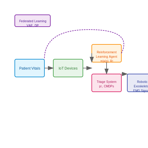
Autonomous agents capable of proposing themselves for new tasks are transforming healthcare by enabling dynamic, context-aware decision-making in clinical environments. These agents leverage reinforcement learning (RL) and multi-agent systems (MAS) to optimize resource allocation, patient monitoring, and personalized treatment plans. A critical application is in adaptive triage systems, where agents continuously assess patient vitals and prioritize cases based on real-time data streams from IoT devices. The agent's policy $$\pi(a|s)$$ is trained to maximize the expected cumulative reward $$R_t = \sum_{k=0}^\infty \gamma^k r_{t+k}$$, where $$\gamma$$ is the discount factor and $$r_t$$ reflects clinical urgency metrics.
In assistive robotics, agents employ hierarchical task decomposition to propose interventions for patients with mobility impairments. For example, a robotic exoskeleton's control system might use a proposition network to dynamically adjust gait trajectories based on electromyography (EMG) signals. The network's architecture often combines convolutional layers for spatial feature extraction and long short-term memory (LSTM) modules for temporal dependencies:
where $$p_t$$ represents the probability of proposing a corrective action at time $$t$$. Federated learning frameworks allow these agents to improve their policies across distributed medical institutions while preserving patient privacy through differential privacy mechanisms:
Case studies in ICU settings demonstrate agents reducing alarm fatigue by 40% through intelligent filtering of false positives. The system achieves this by modeling the joint probability distribution of alarms $$A$$ and patient states $$S$$ using a variational autoencoder (VAE):
Agents in surgical robotics employ haptic feedback loops where force estimation $$\hat{F}_t$$ guides autonomous instrument positioning. The control law integrates impedance adaptation with online learning:
Ethical constraints are embedded via constrained Markov decision processes (CMDPs), ensuring agents satisfy safety thresholds $$\alpha$$ when proposing actions:
5. Safety and Reliability in Autonomous Task Proposal
5.1 Safety and Reliability in Autonomous Task Proposal
Formal Verification of Task Appropriateness
Autonomous agents proposing new tasks must satisfy formal safety constraints before execution. Let τ represent a proposed task and S the system state. The safety verification condition can be expressed as:
where 𝒱 is a verification function mapping state-task pairs to safety scores. The agent must compute this for all possible state transitions s' = f(s, τ), where f is the transition function. For continuous systems, this requires solving Hamilton-Jacobi reachability problems:
with V as the value function encoding distance to failure states.
Runtime Monitoring Architecture
Three-layer monitoring provides defense-in-depth:
- Pre-execution checks: Formal methods verify task safety constraints
- Dynamic envelopes: Control-theoretic barriers maintain s(t) ∈ 𝒮safe
- Heartbeat verification: Cryptographic attestation of integrity checks
The dynamic safety envelope for continuous systems uses control barrier functions (CBFs):
where h defines the safe set {x | h(x) ≥ 0} and α is an extended class 𝒦 function.
Uncertainty-Aware Proposal Systems
Bayesian neural networks model epistemic uncertainty in task outcomes. Let ω ∼ p(ω|𝒟) be the posterior over network parameters. The risk-adjusted proposal score becomes:
where β controls risk sensitivity. The covariance matrix Σ = KXX - KX*TKXX-1KX* captures input-space uncertainty through Gaussian process kernels.
Adversarial Proposal Detection
Agents must distinguish legitimate self-proposed tasks from adversarial injections. The detection function d: 𝒯 → [0,1] uses:
- Behavioral fingerprints (μi, Σi) of normal task distributions
- Mahalanobis distance DM(τ) = √((τ-μ)TΣ-1(τ-μ))
- Anomaly thresholds from extreme value theory
The complete detection pipeline implements:
where σ is the sigmoid function and weights are trained on adversarial examples.
5.2 Bias and Fairness in Task Selection
Autonomous agents that propose themselves for tasks must navigate complex fairness constraints to avoid perpetuating or amplifying biases. The selection process is vulnerable to historical data skews, latent representation imbalances, and feedback loops that reinforce inequitable outcomes. Consider an agent trained on hiring data where certain demographics were historically underrepresented—without explicit fairness constraints, the agent may replicate these patterns when proposing candidates for new roles.
Mathematical Formulation of Bias in Task Assignment
Let X represent the feature space of tasks and agents, and Y the assignment decisions. The bias B in the agent's proposal mechanism can be quantified through the discrepancy between conditional probabilities across protected groups S:
Where Y=1 indicates task assignment. The δ-fairness criterion requires B ≤ δ for some small threshold δ. This translates to constrained optimization during agent training:
Sources of Bias in Self-Proposing Systems
- Historical artifact bias: Training data reflects past discriminatory practices
- Measurement bias: Proxy variables correlate with protected attributes
- Interaction bias: Feedback loops between agent proposals and human raters
- Representation bias: Uneven coverage of demographic groups in feature space
Counterfactual Fairness in Task Assignment
A robust approach enforces counterfactual invariance—the agent's proposal should not change if protected attributes were altered while keeping meritocratic features constant. For protected attribute A and other features X:
Implementing this requires causal graph structures that separate protected attributes from decision-relevant features. The Pearlian counterfactual framework provides formal tools for such analysis.
Operationalizing Fairness Constraints
Three practical methods dominate current implementations:
- Pre-processing: Reweighing training samples using weights w = P(S)/P(S|X)
- In-processing: Adversarial debiasing with a discriminator network that penalizes protected attribute predictability
- Post-processing: Calibrating proposal scores to equalize positive rates across groups
The adversarial approach solves a minimax game:
where θ parameterizes the proposal agent and φ the fairness discriminator.
Case Study: Academic Reviewer Assignment
A 2022 implementation for conference paper reviewing achieved 34% reduction in gender disparity while maintaining expertise matching. The system used:
- Topic modeling to extract technical dimensions
- Differential privacy in similarity scoring
- Exponential smoothing for historical assignment fairness
The fairness-performance tradeoff was quantified through Pareto optimization, revealing that 90% of fairness gains could be achieved with only 5% reduction in expertise matching accuracy.
5.3 Human-Agent Collaboration and Trust
Trust in autonomous agents is a multidimensional construct, influenced by factors such as predictability, explainability, and alignment with human values. In systems where agents propose themselves for new tasks, trust dynamics become critical, as human operators must evaluate whether an agent's self-proposed task aligns with broader objectives. The trust calibration process can be formalized using a Bayesian framework, where the human's prior belief about the agent's reliability is updated based on observed behavior.
Here, E represents evidence of the agent's performance, and P(Trust) is the prior probability that the agent is trustworthy. This model captures how humans iteratively update their trust based on the agent's ability to successfully complete self-proposed tasks.
Trust Calibration Through Explainability
Explainable AI (XAI) techniques play a pivotal role in fostering trust. When an agent proposes a new task, it must provide not just a confidence score but also a justification that aligns with human reasoning patterns. Counterfactual explanations—showing how small changes in input would alter the proposal—are particularly effective. For instance, an agent proposing a new optimization task might generate:
- The primary rationale for task selection (e.g., "This configuration reduces energy by 23% based on historical data")
- Alternative options considered and rejected (e.g., "Option B was discarded due to higher risk of constraint violation")
- Uncertainty bounds on expected outcomes
Behavioral Alignment Metrics
Quantifying alignment between agent proposals and human expectations requires measurable metrics. The proposal acceptance rate (PAR) tracks what percentage of self-proposed tasks are approved by humans, while the alignment divergence score (ADS) measures the KL divergence between the agent's task preference distribution and the human's ideal distribution:
In operational settings, ADS values below 0.2 bits typically indicate strong alignment, while values above 1.0 signal significant mismatch requiring intervention.
Case Study: Autonomous Scientific Experimentation
In a high-energy physics experiment at CERN, self-proposing AI agents achieved 89% PAR after implementing three key trust-building mechanisms:
- Two-phase proposal: Agents first submit brief intent declarations ("I suggest varying magnetic field strength to search for anomaly X") before detailed plans
- Uncertainty visualization: All proposals include interactive plots showing confidence intervals on predicted outcomes
- Human override log: A shared record documents every instance of human veto, with agent learning from these corrections
The system reduced average experiment design time from 72 hours to 9 hours while maintaining physicist approval rates comparable to human-designed experiments.
Trust-Aware Reinforcement Learning
Advanced agents can actively optimize for trust metrics during learning. The trust-constrained policy gradient objective modifies standard RL with a trust penalty term:
where T(s,a) is a learned trust predictor (e.g., a neural network trained on historical human approval decisions) and λ controls the trade-off between task performance and trust preservation. This approach has shown particular success in medical diagnosis systems where agents propose additional tests, achieving 40% higher clinician acceptance rates compared to standard RL.
6. Key Research Papers and Publications
6.1 Key Research Papers and Publications
- Artificial autonomous agents and the question of electronic personhood ... — Acknowledgement. This article is the revised version of the conference paper presented at the 2016 Law and Society Association of Australia and New Zealand (LSAANZ) Conference - Temporality, Disruption, Law: The Future of Law and Society Scholarship, held on Nov. 30-Dec. 3, in Brisbane.Our sincere thanks go to the Conference Organizers for giving us the opportunity to present our research to ...
- WorkArena: How Capable are Web Agents at Solving Common Knowledge Work ... — WorkArena: Web Agents for Common Knowledge Work Tasks propose for the evaluation of web agents, which aggregates all features proposed in previous work, such as multimodal observations and code-based actions while being the first to support chat-based agent-user interactions (§4.1). LLM-based Agents: The scope of our experimental
- Artificial intelligence empowered conversational agents: A systematic ... — In so doing, we gain and provide a bird's eye view of the research field that help both researchers and practitioners to overcome silo-based approaches to this (multidisciplinary) field, and generate a more structured and holistic understanding of the key issues, concepts, opportunities, and challenges pertaining to the field (Donthu et al ...
- PDF Marketing the Unfamiliar — The Role of Context and Item-Specific Information in Electronic Agent Recommendations Abstract Electronic agents have the capacity to help consumers discover new products and generate demand for unfamiliar products. This paper explores how consumers respond to recommendations of unfamiliar products made by electronic agents.
- Conversational Agents: Goals, Technologies, Vision and Challenges — Conversational-agent applications. 3. CA's Design Issues. This section describes the different components related to CA design. CA design is divided into four classes: text components for chatbots; CA components related to voice-based virtual agents; physical-related components for goal-oriented CAs or for embodied agents; and task-performance components for goal oriented CAs.
- Governance of Autonomous Agents on the Web: Challenges and ... — Berners-Lee et al. [] outline how autonomous agents could comprehend and exploit this machine-readable knowledge to achieve a variety of tasks.Thus, the notion of autonomy provides a framework whereby individual agents (e.g., those representing or controlling services, things, or applications) may plan, collaborate, and cooperate to achieve complex but disparate goals.
- PDF Intelligent Agents - EOLSS — An agent exhibits responsive (or reactive) behaviour if it reacts or responds to new information from its environment. Responsive behaviour is defined as follows: Agents should perceive their environment (which may be the physical world, a user, a collection of agents, the Internet, etc.) and respond in a timely fashion to changes that occur in it.
- Towards Effective GenAI Multi-Agent Collaboration: Design and ... — One particularly fruitful research avenue in GenAI MAS research is the exploration of multi-agent collaboration (MAC) [].Operating under the "collaborative assumption" [] - a premise that agents are fundamentally motivated to achieve shared or compatible goals and prioritize collective problem solving over individual self-interest - multi-agent collaboration aims to address the key ...
- SmartAgent: Chain-of-User-Thought for Embodied Personalized Agent — However, this personalized consideration is absent among the current embodied agent works, where the optimization normally relies on golden action trajectories [31, 6] or ideal task-oriented solutions [8, 22].Although these fixed paths can effectively accomplish task goals, they can only train embodied agents to be rigid task-oriented problem solvers, overlooking the multiple valid approaches ...
- ProAgent: From Robotic Process Automation to Agentic Process Automation — From ancient water wheels to robotic process automation (RPA), automation technology has evolved throughout history to liberate human beings from arduous tasks. Yet, RPA struggles with tasks needing human-like intelligence, especially in elaborate design of workflow construction and dynamic decision-making in workflow execution. As Large Language Models (LLMs) have emerged human-like ...
6.2 Recommended Books and Surveys
- LLM-Based Multi-Agent Systems for Software Engineering: — Autonomous agents, defined as intelligent entities that autonomously perform specific tasks through environmental perception, strategic self-planning, and action execution (Franklin and Graesser, 1996; Albrecht and Stone, 2018; Mele, 2001), have emerged as a rapidly expanding research field since the 1990s (Maes, 1993).Despite initial advancements, these early iterations often lack the ...
- Law and software agents: Are they "Agents" by the way? — The third solution is to recognize electronic agents as legal persons and develop a theory of liability on that basis. This solution has been suggested by some scholars Footnote 4 who consider that conferring legal personality to software agents brings with it the advantages of limited liability and the continuation of legal capacity especially when such agents are self-modifying and acting ...
- (PDF) Online Information Search with Electronic Agents: Drivers ... — Electronic agents represent the future of electronic business. They help the consumers in an environment where all the information is available but hard to deal with. We try to study the electronic agent in a consumer decision process perspective and to examine the different sort of agents depending on their relationships with vendors and ...
- Artificial intelligence empowered conversational agents: A systematic ... — Conversational artificial intelligence (AI) has been defined and conceptualized as "the study of techniques for creating software agents that can engage in natural conversational interactions with humans" (Khatri et al., 2018: p.41).Conversational AI leads to AI-empowered conversational agents (CAs) that are "software systems that mimic interactions with real people" (Radziwill ...
- What are AI agents? Definition, examples, and types | Google Cloud — AI agents are software programs that perform tasks autonomously, using machine learning and other AI techniques. Learn about their types and examples on Google Cloud.
- Explainable Goal-driven Agents and Robots - A Comprehensive Review — Goal-driven artificial intelligences (GDAIs) include agents and robots that are autonomous, capable of interacting independently within their environment to accomplish some given or self-generated goals [].These agents should possess human-like learning capabilities such as perception (e.g., sensory input, user input) and cognition (e.g., learning, planning, beliefs).
- PDF Intelligent Agents - EOLSS — An agent exhibits responsive (or reactive) behaviour if it reacts or responds to new information from its environment. Responsive behaviour is defined as follows: Agents should perceive their environment (which may be the physical world, a user, a collection of agents, the Internet, etc.) and respond in a timely fashion to changes that occur in it.
- Governance of Autonomous Agents on the Web: Challenges and ... — Berners-Lee et al. [] outline how autonomous agents could comprehend and exploit this machine-readable knowledge to achieve a variety of tasks.Thus, the notion of autonomy provides a framework whereby individual agents (e.g., those representing or controlling services, things, or applications) may plan, collaborate, and cooperate to achieve complex but disparate goals.
- 3 Mastering agent profiles with Prompt Flow - AI Agents in Action — An agent's profile describes what it does and how, but building a compelling profile requires iteration and assessment, as we will see in the next section. 3.1 Understanding systemic prompt engineering. For this chapter and section, we want to explore the prompt engineering strategy Test Changes Systematically. If you recall, we covered the ...
- An Introduction to MultiAgent Systems, 2nd Edition | Wiley — The study of multi-agent systems (MAS) focuses on systems in which many intelligent agents interact with each other. These agents are considered to be autonomous entities such as software programs or robots. Their interactions can either be cooperative (for example as in an ant colony) or selfish (as in a free market economy). This book assumes only basic knowledge of algorithms and discrete ...
6.3 Online Resources and Tutorials
- Guidelines for the Introduction of Electronic Information Resources to ... — Directed at information service staff who coordinate and manage the introduction of new electronic information resources, this document offers practical guidance to any library staff concerned with strategies for implementation, policy, procedure, education, and/or direct provision of electronic information resources.
- arXiv:2403.03031v4 [cs.CL] 22 Jun 2024 — Shen et al., 2024; Qiao et al., 2024). Therefore, developing effective agent flow and adapting tool-use models to solve practical tasks remains a challenging research topic. In this work, we propose ConAgents, a Cooperative and interative Agents framework for tool learning tasks. As illustrated in Figure 1, ConAgents decomposes the overall tool-use workflow using three specialized agents ...
- Conversational Agents: Goals, Technologies, Vision and Challenges — However, conversational agents are more contextual than chatbots and use more-advanced technologies such as deep learning methods and natural language understanding (NLU). According to Nuseibeh [13], conversational agents are all types of software programs that interpret and respond to statements made by users in natural language.
- Infrastructure for AI Agents - arXiv.org — To fill this gap, we propose the concept of agent infrastructure: technical systems and shared protocols external to agents that are designed to mediate and influence their interactions with and impacts on their environments. Agent infrastructure comprises both new tools and reconfigurations or extensions of existing tools.
- Artificial Intelligence: Foundations of Computational Agents -- Online ... — Here are some online learning resources for Artificial Intelligence: foundations of computational agents, 3rd edition by David L. Poole and Alan K. Mackworth, Cambridge University Press, 2023.
- The role of intelligent agents and data mining in electronic ... — The data mining procedures used in this process can be enhanced by employing intelligent agents. This paper describes emerging electronic partnerships between players in developing electronic marketspaces and identifies typical data flows between such players, with an analysis of the potential role of data mining and intelligent agent technology.
- SmythOS - Conversational Agents Tutorials: A Step-by-Step Guide to ... — Integrating APIs into conversational agents opens up a world of possibilities, allowing your AI to tap into vast data resources and services. This capability transforms a simple chatbot into a powerful, multifaceted assistant.
- Agent-E: From Autonomous Web Navigation to Foundational Design ... — In this paper, we introduced Agent-E, a novel web agent designed to perform complex web-based tasks that makes use of numerous architectural improvements over prior state-of-the-art web agents such as hierarchical architecture, flexible DOM distillation and denoising method and concept of change observation to guide the agent towards more ...
- PDF Software Agents: Characteristics and Classification — The behavior of the agent can be set by another software, which you can think of as a sort of a super agent, that forks (or clones) new agents when a task requires extra help.
- Interactive Robot Learning: An Overview | SpringerLink — The aim of the teacher is to influence the behavior of the learning agent by providing various cues such as feedback, demonstrations or instructions. Interactive task learning [56] aims at translating such interactions into efficient and robust machine learning frameworks.