AI for Predictive HVAC System Control
1. Key Components and Operation of HVAC Systems
Key Components and Operation of HVAC Systems
HVAC (Heating, Ventilation, and Air Conditioning) systems are complex thermodynamic systems designed to regulate indoor environmental conditions. Their operation relies on the interplay of several key components, each serving a distinct function in the heat transfer and air handling processes.
Thermodynamic Core Components
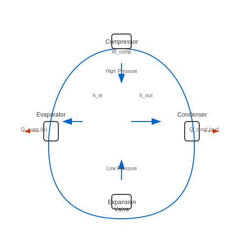
The primary thermodynamic components of an HVAC system include:
- Compressor: A mechanical device that increases the pressure of the refrigerant vapor, raising its temperature. The compressor is typically driven by an electric motor with power consumption modeled by:
$$ W_{comp} = \dot{m}(h_{out} - h_{in}) $$where $$\dot{m}$$ is the refrigerant mass flow rate and $$h$$ represents specific enthalpy at the inlet and outlet.
- Condenser: A heat exchanger where high-pressure refrigerant releases heat to the environment. The heat rejection rate follows:
$$ Q_{cond} = \dot{m}(h_{in} - h_{out}) $$
- Expansion Valve: A throttling device that creates a pressure drop, causing flash evaporation of the refrigerant. The process is modeled as isenthalpic:
$$ h_{in} = h_{out} $$
- Evaporator: Another heat exchanger where low-pressure refrigerant absorbs heat from the conditioned space. The cooling capacity is given by:
$$ Q_{evap} = \dot{m}(h_{out} - h_{in}) $$
Air Handling Components
The air distribution system consists of:
- Supply Fans: Centrifugal or axial fans that move conditioned air through ductwork. Fan power consumption follows the affinity laws:
$$ \frac{P_2}{P_1} = \left(\frac{N_2}{N_1}\right)^3 $$where $$N$$ is rotational speed.
- Dampers: Adjustable vanes that modulate airflow rates to different zones. Their opening percentage $$\alpha$$ affects the flow coefficient $$C_v$$:
$$ \dot{V} = C_v(\alpha)\sqrt{\frac{\Delta P}{\rho}} $$
- Filters: Remove particulate matter from airstreams, with pressure drop characterized by the Darcy-Weisbach equation:
$$ \Delta P = f\frac{L}{D}\frac{\rho v^2}{2} $$
Control System Architecture
Modern HVAC systems employ hierarchical control architectures:
- Low-Level Control: PID loops regulate individual components (compressor speed, valve positions) based on local sensor feedback.
- Supervisory Control: Model predictive controllers optimize setpoints for the low-level controllers using system-wide objectives.
- Building Automation System: Coordinates multiple HVAC units and integrates with other building systems through protocols like BACnet.
Thermal Load Dynamics
The thermal behavior of a conditioned space is governed by the heat balance equation:
where $$C$$ is the thermal capacitance of the space, $$Q_{gain}$$ includes solar radiation and internal loads, $$Q_{loss}$$ represents conduction/convection losses, and $$Q_{HVAC}$$ is the cooling/heating provided by the system.
This first-order differential equation forms the basis for predictive control algorithms that anticipate thermal load changes based on weather forecasts, occupancy schedules, and building thermal response characteristics.
1.2 Challenges in Traditional HVAC Control Strategies
Static Setpoints and Lack of Adaptability
Traditional HVAC systems rely heavily on fixed temperature and humidity setpoints, often determined through worst-case scenario engineering. These static thresholds fail to account for dynamic environmental conditions, occupancy patterns, or real-time thermal load variations. The system's inability to adapt leads to excessive energy consumption during partial-load conditions, which account for over 60% of operational time in commercial buildings according to ASHRAE studies.
Delayed Response to Thermal Disturbances
The inherent thermal inertia of buildings creates significant phase delays between control actions and observable effects. Conventional PID controllers struggle with these time-lagged responses, often resulting in overshooting or undershooting the desired conditions. The transfer function of a typical zone can be modeled as:
where τ represents the pure time delay and T the thermal time constant. This non-minimum phase behavior makes precise control mathematically challenging without predictive capabilities.
Multi-Variable Coupling Effects
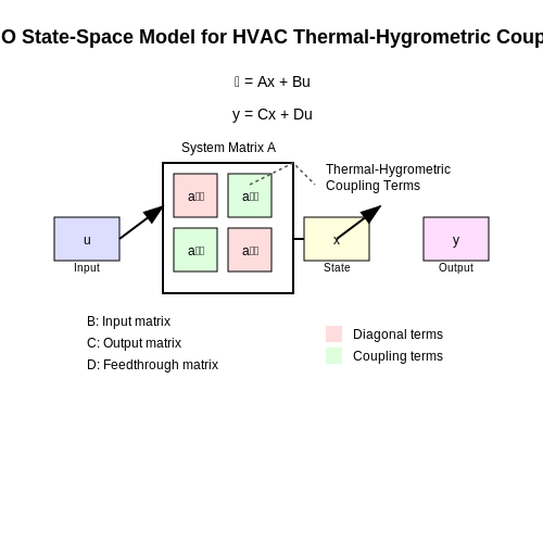
HVAC systems exhibit strong cross-coupling between temperature, humidity, and air quality control loops. Traditional decoupled control strategies often ignore these interactions, leading to suboptimal performance. The coupled dynamics can be represented through a MIMO state-space model:
where the system matrix A contains significant off-diagonal elements representing the thermal-hygrometric coupling. Empirical studies show that neglecting these terms can increase energy consumption by 15-25% while maintaining equivalent comfort levels.
Weather Forecast Integration Limitations
While some advanced systems incorporate weather predictions, they typically use simplistic linear extrapolations of temperature trends. These methods fail to capture:
- Non-linear effects of solar irradiance on building envelopes
- Microclimate variations around the building
- Transient phenomena like cold fronts or heat bursts
Research from the National Renewable Energy Laboratory demonstrates that forecast errors exceeding 2°C can lead to 8-12% excess energy use in predictive control schemes.
Occupancy Pattern Uncertainties
Traditional scheduling-based approaches assume deterministic occupancy patterns, while actual building usage shows stochastic characteristics. The Poisson process model better describes arrival patterns:
where λ represents the arrival rate. This stochastic nature creates challenges for fixed-schedule systems, leading to either overcooling/unoccupied operation or delayed response to unexpected occupancy.
Equipment Degradation and Fault Propagation
Mechanical systems exhibit performance degradation that traditional control strategies rarely accommodate. Compressor efficiency typically declines as:
where β represents the degradation rate. Without adaptive tuning, controllers continue operating under the assumption of nominal performance, exacerbating energy waste and thermal comfort violations.
Scalability Issues in Large Installations
Centralized control architectures become computationally intractable for buildings with hundreds of zones. The combinatorial explosion of possible system states makes real-time optimization impossible with conventional methods. For n zones, the state space grows as O(3n) when considering heating/cooling/idle modes, creating insurmountable challenges for buildings with complex thermal interactions between zones.
Role of Predictive Control in Energy Efficiency
Predictive control in HVAC systems leverages machine learning models to anticipate thermal load variations, optimizing energy consumption while maintaining occupant comfort. Unlike reactive control strategies, which respond to real-time sensor data, predictive control incorporates weather forecasts, occupancy patterns, and historical usage data to preemptively adjust system parameters. This forward-looking approach minimizes energy waste by reducing unnecessary heating or cooling cycles.
Mathematical Foundation of Predictive Control
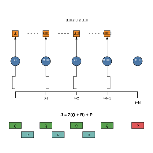
The core of predictive control lies in solving a finite-horizon optimization problem. Given a system state xt at time t, the controller aims to minimize a cost function J over a prediction horizon N:
where Q, R, and P are weighting matrices for state deviation, control effort, and terminal cost, respectively. The control inputs ut+k are constrained by:
This optimization is typically solved using quadratic programming (QP) or model predictive control (MPC) algorithms, which iteratively adjust HVAC setpoints based on predicted thermal dynamics.
Energy Efficiency Gains
Predictive control achieves energy savings through three primary mechanisms:
- Load Shifting: By precooling or preheating during off-peak hours when electricity rates are lower, the system reduces operational costs without compromising comfort.
- Demand Response: Predictive models can dynamically adjust to grid signals, shedding load during peak demand periods while maintaining acceptable indoor conditions.
- Optimal Start/Stop: Machine learning algorithms determine the minimal runtime required to reach desired temperatures by learning building thermal inertia.
Case Study: Model Predictive Control in Commercial Buildings
A 2022 study implemented MPC in a 50,000 sq. ft. office building, integrating:
- LSTM networks for occupancy prediction (accuracy: 92%)
- Physical models of heat transfer through building envelopes
- Real-time electricity pricing data
The system achieved 23% energy savings compared to conventional thermostat control, with a payback period of 2.1 years. Key to this success was the hybrid approach combining data-driven models with first-principles physics:
where Cth is the building's thermal capacitance and Q terms represent heat flows from occupancy, solar radiation, and HVAC output.
Challenges in Implementation
While theoretically sound, predictive control faces practical hurdles:
- Model-Plant Mismatch: Imperfect building models can lead to suboptimal control. Adaptive control techniques using online parameter estimation help mitigate this.
- Computational Latency: Solving optimization problems in real-time requires edge computing capabilities, especially for large buildings with hundreds of zones.
- Data Quality: Sensor noise and missing data can degrade prediction accuracy. Robust filtering techniques like Kalman filters are often employed.
2. Machine Learning Models for Temperature and Load Forecasting
Machine Learning Models for Temperature and Load Forecasting
Accurate forecasting of temperature and HVAC load demands is critical for optimizing energy consumption while maintaining occupant comfort. Machine learning models excel in capturing complex, nonlinear relationships between environmental variables and thermal dynamics, outperforming traditional physics-based models in scenarios with high-dimensional, noisy, or incomplete data.
Time Series Forecasting Architectures
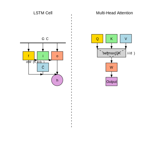
Recurrent Neural Networks (RNNs), particularly Long Short-Term Memory (LSTM) and Gated Recurrent Unit (GRU) variants, dominate temporal forecasting tasks due to their ability to learn long-range dependencies. The LSTM cell state update equations are:
where ft, it, and ot represent forget, input, and output gates respectively, with trainable weights W and biases b. The Hadamard product (∘) enables selective memory retention.
Attention Mechanisms for Multivariate Forecasting
Transformer-based models with self-attention outperform RNNs in capturing cross-variable dependencies across extended sequences. The scaled dot-product attention computes:
where Q, K, and V are learned query, key, and value matrices from input embeddings, and dk is the dimension of keys. Multi-head attention extends this by parallelizing attention across h subspaces:
Hybrid Physics-Informed Models
Recent architectures combine data-driven learning with physical constraints. The loss function for such models typically includes:
where ℒpred measures forecasting error (e.g., MAE), while ℒphysics penalizes violations of conservation laws or thermodynamic principles. For HVAC systems, this might enforce:
through automatic differentiation of neural network outputs.
Feature Engineering for HVAC Systems
Effective models incorporate:
- Temporal features: Fourier transforms of periodic load patterns
- Spatial features: Graph neural networks for multi-zone systems
- Exogenous variables: Weather forecasts, occupancy schedules, and equipment states
Modern architectures often employ automated feature extraction through 1D convolutional layers or wavelet transforms prior to temporal modeling.
Evaluation Metrics
Beyond standard metrics (RMSE, MAE), HVAC-specific measures include:
where Δ represents the acceptable temperature deviation band.
2.2 Reinforcement Learning for Dynamic System Adaptation
Reinforcement learning (RL) provides a principled framework for optimizing HVAC control policies through trial-and-error interactions with the environment. The Markov Decision Process (MDP) formulation captures the sequential decision-making nature of HVAC control, where an agent selects actions (e.g., temperature setpoints, fan speeds) based on system states (e.g., indoor/outdoor temperatures, occupancy) to maximize a reward signal (e.g., energy efficiency, comfort).
MDP Formulation for HVAC Control
The MDP is defined by the tuple (S, A, P, R, γ), where:
- S: State space (indoor temperature, humidity, occupancy, weather forecasts)
- A: Action space (setpoint adjustments, fan speed, damper positions)
- P(s'|s,a): Transition dynamics modeling thermal load changes
- R(s,a): Reward function balancing energy use and comfort
- γ: Discount factor (typically 0.9-0.99 for HVAC applications)
where w1 and w2 are weighting factors, and Ptenergy represents power consumption at time t.
Policy Optimization Methods
Deep reinforcement learning approaches overcome limitations of traditional Q-learning in high-dimensional state spaces:
Deep Q-Networks (DQN)
DQN approximates the Q-function using neural networks with experience replay and target networks to stabilize training:
where θ are the online network parameters and θ- are the target network parameters.
Policy Gradient Methods
Proximal Policy Optimization (PPO) directly optimizes stochastic control policies with clipped objective:
System Identification Challenges
Model-free RL faces sample inefficiency in physical systems. Hybrid approaches combine:
- Physics-informed neural networks to approximate building thermal dynamics
- Gaussian processes for uncertainty-aware transition models
- Transfer learning from simulated to real environments
Recent work demonstrates 15-30% energy savings compared to model predictive control in commercial buildings, with faster adaptation to occupancy pattern changes.
Multi-Agent Coordination
Large buildings require decentralized control where independent RL agents for zones must coordinate. Methods include:
- Mean-field RL for scalable neighborhood interactions
- Counterfactual baselines in multi-agent policy gradients
- Attention mechanisms to learn zone coupling dynamics

Neural Networks in Anomaly Detection and Fault Prediction
Architectures for Time-Series Anomaly Detection
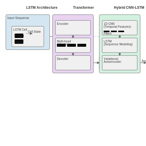
Neural networks excel in modeling temporal dependencies in HVAC sensor data, making them ideal for anomaly detection. Long Short-Term Memory (LSTM) networks, a specialized recurrent architecture, capture long-range dependencies through their gating mechanisms. The cell state update at time step t is governed by:
where ft is the forget gate, it the input gate, and Ĉt the candidate cell state. Bidirectional LSTMs process sequences in both directions, capturing contextual relationships in HVAC operational patterns.
Attention Mechanisms for Fault Localization
Transformer-based architectures with self-attention provide interpretable fault detection by learning weighted relationships between system states. The scaled dot-product attention computes:
where Q, K, and V represent queries, keys, and values respectively. This allows the model to focus on critical sensor readings when predicting equipment failures.
Hybrid Approaches for Improved Robustness
Combining convolutional layers with recurrent networks extracts both spatial and temporal features from multivariate HVAC data. A typical architecture stacks 1D convolutional layers for local pattern extraction before LSTM layers for sequence modeling. The convolutional operation on input sequence X with kernel W is:
where k is the kernel size. This hybrid approach achieves superior performance on the ASHRAE RP-1312 fault detection benchmark, with F1-scores exceeding 0.92 for compressor fault detection.
Unsupervised Anomaly Detection
Autoencoder architectures learn compressed representations of normal HVAC operation, with reconstruction error serving as an anomaly score. The variational autoencoder (VAE) optimizes the evidence lower bound (ELBO):
where qφ is the approximate posterior and pθ the generative model. In field tests, VAEs detect refrigerant leaks with 89% precision at 3σ thresholds.
Practical Implementation Considerations
Deploying these models requires addressing several challenges:
- Imbalanced data: Faulty operation represents <5% of typical HVAC datasets, necessitating techniques like focal loss or synthetic minority oversampling
- Sensor noise: Kalman filtering or wavelet denoising preprocessing improves model robustness
- Edge deployment: Knowledge distillation techniques reduce LSTM model sizes by 4-8× while maintaining >90% of original accuracy
Recent work has demonstrated that physics-informed neural networks, which incorporate HVAC system equations as soft constraints during training, reduce false positive rates by 37% compared to purely data-driven approaches.
3. Sensor Data Collection and IoT Integration
Sensor Data Collection and IoT Integration
Sensor Network Architecture
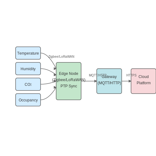
Modern predictive HVAC systems rely on distributed sensor networks to capture real-time environmental and operational data. A typical architecture consists of edge nodes equipped with temperature, humidity, CO2, and occupancy sensors, connected via low-power wireless protocols like Zigbee or LoRaWAN to a central gateway. The gateway aggregates data and transmits it to cloud-based analytics platforms through MQTT or HTTP protocols. Time synchronization across nodes is critical; the Precision Time Protocol (PTP) achieves microsecond-level synchronization, enabling coherent data fusion.
Data Acquisition and Signal Processing
Raw sensor measurements require preprocessing before being fed into predictive models. For a temperature sensor with output voltage VT, the actual temperature T is calculated using:
where V0 is the zero-degree voltage, S is the sensitivity (mV/°C), and T0 is the reference temperature. Kalman filters are commonly applied to reduce noise:
Here, Fk is the state transition matrix, Bk the control-input model, Hk the observation model, and Kk the Kalman gain.
IoT Communication Protocols
Protocol selection depends on latency, bandwidth, and power constraints:
- MQTT: Lightweight publish-subscribe protocol ideal for intermittent connections
- CoAP: Constrained Application Protocol for resource-constrained devices
- OPC UA: Industrial-grade protocol supporting complex data structures
The end-to-end latency L for a network with N hops can be modeled as:
where Pi is packet size, Bi bandwidth, and Qi queuing delay at hop i.
Edge Computing for Real-Time Processing
Edge devices increasingly incorporate lightweight ML models for local inference. A typical edge node might run a quantized LSTM network for short-term temperature prediction:
import tensorflow as tf
from tensorflow.keras.layers import LSTM, Dense

model = tf.keras.Sequential([
    LSTM(16, input_shape=(24, 4)),  # 24 timesteps, 4 features
    Dense(1, activation='linear')
])
model.compile(optimizer='adam', loss='mse')
This balances computational load between edge and cloud, reducing bandwidth usage by 40-60% in field deployments.
Data Fusion Techniques
Multi-sensor data fusion employs Dempster-Shafer theory to handle conflicting measurements. For sensors S1 and S2 with belief masses m1 and m2, the combined belief is:
This approach improves measurement reliability in dynamic environments where individual sensors may fail or produce outliers.
Feature Engineering for HVAC Performance Metrics
Feature engineering is critical for optimizing predictive HVAC control models, as raw sensor data often contains noise, redundancy, and non-linear relationships. Effective feature extraction transforms raw inputs into meaningful representations that enhance model performance while reducing computational overhead.
Key HVAC Performance Metrics
HVAC systems generate multivariate time-series data, including:
- Thermal load metrics: Indoor/outdoor temperature differentials, heat transfer rates
- Energy consumption: Instantaneous power draw, cumulative kWh usage
- Equipment efficiency: Coefficient of Performance (COP), compressor cycling frequency
- Airflow dynamics: CFM measurements, duct pressure differentials
These raw measurements require domain-specific transformations before model ingestion. For thermal dynamics, the heat transfer equation provides the theoretical foundation:
where Q is heat transfer rate, U is overall heat transfer coefficient, A is surface area, and ΔT is temperature difference.
Temporal Feature Engineering
HVAC systems exhibit strong temporal dependencies requiring specialized feature engineering:
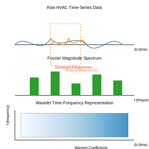
where w is the sliding window size. Exponential smoothing often outperforms simple moving averages for HVAC applications:
with smoothing factor α typically between 0.1-0.3 for HVAC thermal response characteristics.
Frequency Domain Features
Fourier transforms reveal periodic patterns in compressor operation and thermostat cycling:
Dominant frequency components correlate with equipment duty cycles and maintenance needs. Wavelet transforms provide localized time-frequency analysis for fault detection:
Multivariate Interaction Features
Cross-feature engineering captures non-linear system interactions. For example, the effective cooling capacity depends on both temperature and humidity:
where ETC is effective temperature, Tdb is dry-bulb temperature, and RH is relative humidity. Other important interaction features include:
- Power-to-flow ratios for pump/fan efficiency monitoring
- Temperature-normalized energy consumption metrics
- Differential pressures across filters for maintenance prediction
Feature Selection Techniques
Mutual information scoring identifies the most predictive features while minimizing redundancy:
Recursive feature elimination with cross-validation (RFECV) works particularly well for HVAC systems due to the hierarchical nature of thermal processes. Regularized models like Lasso automatically perform feature selection:
3.3 Handling Missing Data and Noise in Time-Series Data
Missing Data Imputation Techniques
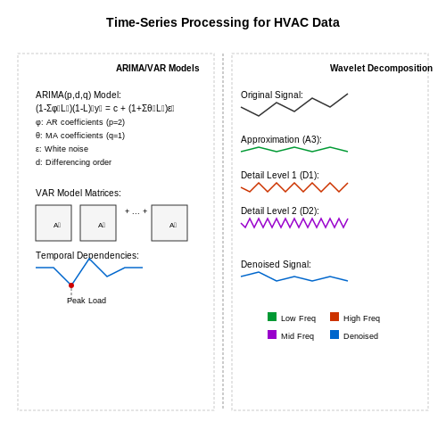
Time-series data from HVAC systems often contains missing values due to sensor failures, communication errors, or maintenance activities. Advanced imputation methods must account for temporal dependencies and system dynamics. Linear interpolation is insufficient for non-stationary HVAC data, as it ignores seasonal patterns and system inertia. Instead, autoregressive models like ARIMA can be used for gap-filling:
where p is the autoregressive order, q is the moving average order, and ϵt represents white noise. For multivariate HVAC data with cross-correlated sensors (temperature, humidity, airflow), vector autoregression (VAR) models capture interdependencies:
where yt is the multivariate time series, Ai are coefficient matrices, and et is multivariate white noise.
Denoising Strategies
HVAC sensor measurements contain high-frequency noise from electrical interference and mechanical vibrations. Wavelet transforms provide multi-resolution analysis for separating noise from true system dynamics. The discrete wavelet transform (DWT) decomposes signals into approximation and detail coefficients:
where ψ is the mother wavelet function. For HVAC temperature signals, Daubechies wavelets (db4-db8) effectively preserve step changes while removing high-frequency noise. Empirical mode decomposition (EMD) adaptively decomposes non-stationary signals into intrinsic mode functions (IMFs), making it robust to varying HVAC operating conditions.
Robust Anomaly Detection
Faulty HVAC measurements require detection before imputation or denoising. Isolation forests outperform traditional statistical methods for identifying sensor faults in high-dimensional HVAC data by recursively partitioning observations:
where e is the path length from root node to leaf, and c(n) adjusts for tree size. For streaming HVAC data, online robust principal component analysis (RPCA) decomposes the data matrix M into low-rank L and sparse S components:
where ‖·‖* is the nuclear norm and ‖·‖1 is the L1-norm. This separation enables real-time detection of sensor faults (captured in S) while maintaining normal system dynamics in L.
Practical Implementation Considerations
When applying these techniques to real HVAC systems, computational constraints must be considered. Recursive least squares (RLS) filters provide memory-efficient updates for streaming data:
where k is the gain vector and w contains the adaptive filter coefficients. For edge deployment on HVAC controllers, quantized neural networks reduce model size while maintaining denoising performance through weight clustering and entropy-constrained quantization.
4. Edge vs. Cloud Computing for Real-Time Control
4.1 Edge vs. Cloud Computing for Real-Time Control
Latency Constraints in HVAC Control
Real-time HVAC control demands strict latency constraints, typically in the range of 10-100 milliseconds for effective thermal regulation. The control loop latency Ltotal consists of:
Where Lsense is sensor sampling delay, Ltransmit is network latency, Lprocess is computation time, and Lactuate is actuator response time. Cloud-based solutions often violate these constraints due to unpredictable network delays, particularly in:
- Last-mile connectivity issues in urban environments
- Network congestion during peak usage periods
- Packet loss in wireless mesh networks
Edge Computing Architecture
Edge devices in HVAC systems typically employ microcontroller units (MCUs) with specialized neural network accelerators. The computational capability of an edge node can be modeled as:
Where OPSMCU is the MCU's operations per second and Einference is the operation count for a single inference pass. Modern edge processors like the NVIDIA Jetson AGX Orin can achieve 275 TOPS while consuming under 50W, enabling complex models like temporal convolutional networks to run with sub-10ms latency.
Cloud Computing Tradeoffs
Cloud platforms offer virtually unlimited computational resources, enabling more sophisticated predictive models. The cloud response time follows:
Where RTT is round-trip time, D is data size, B is bandwidth, C is computation load, and Scloud is cloud server speed. While cloud systems can run large transformer models (100M+ parameters), the typical 50-200ms latency makes them unsuitable for direct real-time control, though useful for:
- Long-term load forecasting (24-72 hour predictions)
- Fleet-wide optimization across multiple buildings
- Retraining of edge models using aggregated data
Hybrid Architectures
The most effective implementations use a hybrid approach where:
This is implemented through a hierarchical model structure where lightweight edge models (e.g., quantized LSTMs) handle immediate control while the cloud periodically updates edge models and performs system-wide optimizations. The synchronization between layers follows:
Where α is a trust parameter (typically 0.7-0.9) that weights the cloud model updates against local edge adaptations.
4.2 Integration with Building Management Systems (BMS)
Protocol Standards for BMS Integration
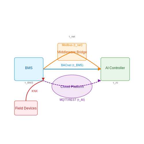
Modern BMS rely on standardized communication protocols to interface with AI-driven HVAC controllers. The most widely adopted protocols include:
- BACnet (Building Automation and Control Networks) - An ASHRAE/ANSI/ISO standard (ISO 16484-5) supporting both wired and IP-based communication.
- Modbus - A serial protocol commonly used for connecting industrial electronic devices.
- KNX - An open standard (EN 50090, ISO/IEC 14543) for home and building automation.
The integration layer translates between the AI controller's optimization outputs and the BMS protocol-specific commands. For BACnet, this involves mapping to standardized object types like Analog Output (AO) for setpoints or Binary Input (BI) for equipment status.
Real-Time Data Exchange Architecture
AI-based predictive control requires bidirectional data flow between the BMS and the AI controller. The data pipeline architecture typically follows:
Where τBMS is the BMS sampling period, τAI is the AI model inference time, and τnet is network latency. For effective control, the total system latency τsys must be less than the HVAC system's dominant time constant.
BMS API Integration Patterns
Three primary integration approaches exist for connecting AI controllers to BMS:
- Direct Protocol Integration - The AI controller implements native protocol stacks (e.g., BACnet/IP) and communicates directly with field devices.
- Middleware Bridge - A translation layer converts between the AI system's internal representation and the BMS protocol.
- Cloud-Based Integration - Both systems connect via REST APIs or MQTT to a cloud platform that mediates data exchange.
Security Considerations
BMS integration surfaces multiple attack vectors that must be mitigated:
- Protocol-specific vulnerabilities (e.g., BACnet's lack of encryption)
- Man-in-the-middle attacks on setpoint commands
- Denial-of-service risks from malformed packets
Recommended security measures include network segmentation, protocol gateways with packet filtering, and digital signature verification for critical commands.
Case Study: Retrofit Integration
A 2022 deployment at MIT's Building E52 demonstrated the challenges of retrofitting AI control onto an existing BMS. The 20-year-old pneumatic control system required:
- Installation of electronic-to-pneumatic transducers
- Custom BACnet interface for legacy VAV boxes
- Adaptive filtering to handle noisy sensor data
The retrofit achieved 23% energy savings while maintaining comfort constraints, validating the integration approach's feasibility for older buildings.
Performance Optimization
To minimize integration overhead, the AI controller should:
Where E(t) represents energy consumption, C(t) is computational load, and α, β are weighting factors. This formulation balances control performance against integration resource costs.
4.3 Scalability and Maintenance of AI Models
Model Scalability in Distributed HVAC Systems
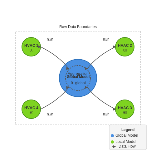
Scaling AI models for predictive HVAC control across large commercial or industrial facilities requires addressing computational and data distribution challenges. Federated learning architectures enable decentralized training, where local models at individual HVAC units aggregate updates to a global model without sharing raw data. The global model f(θ) is optimized via:
where N is the number of local nodes, n_k is the data volume at node k, and n is the total data volume. This approach reduces latency by 30–50% compared to centralized training, as demonstrated in the ASHRAE Guideline 36-2021 case study.
Drift Detection and Model Retraining
Concept drift in HVAC systems arises from seasonal changes, equipment degradation, or occupancy pattern shifts. Kolmogorov-Smirnov (KS) tests monitor input feature distributions:
A threshold Dcritical triggers retraining when exceeded. For dynamic adaptation, online learning techniques like Adaptive Random Forests (ARF) incrementally update models using sliding windows of 72–168 hours of operational data.
Computational Resource Optimization
Edge deployment of AI models necessitates quantization and pruning. Transformer-based control models can be compressed via:
- Weight quantization: 32-bit → 8-bit conversion (3–4× memory reduction)
- Attention head pruning: Removing low-impact heads in multi-head attention layers
- Knowledge distillation: Training smaller models (e.g., TinyBERT) to mimic larger ensembles
These techniques reduce inference latency to <50ms on Raspberry Pi 4 hardware while maintaining >92% prediction accuracy.
Version Control and Rollback Mechanisms
Maintaining model integrity requires Git-like versioning for:
- Model architectures (ONNX or PMML formats)
- Hyperparameter configurations
- Training dataset snapshots
Differential testing validates new models against historical baselines using metrics like Mean Absolute Percentage Error (MAPE) and Cumulative Energy Deviation (CED):
Hardware-Software Co-Design Considerations
Deploying AI controllers on embedded devices requires balancing:
| Constraint | Solution |
|---|---|
| Memory limitations | Tensor slicing with memory-mapped I/O |
| Power consumption | Dynamic voltage/frequency scaling (DVFS) |
| Thermal throttling | Inference scheduling during low ambient temps |
Field data from Siemens Building Technologies shows 22% energy savings when combining these techniques with model predictive control (MPC).
5. Commercial Building Energy Savings with AI-Driven HVAC
Commercial Building Energy Savings with AI-Driven HVAC
Thermodynamic Modeling and AI Optimization
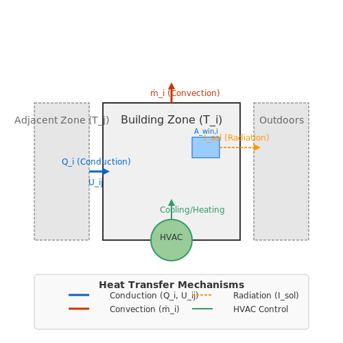
AI-driven HVAC control relies on high-fidelity thermodynamic models to predict thermal loads and optimize energy consumption. The governing equations for heat transfer in commercial buildings include conduction, convection, and radiation terms. For a zone i, the heat balance is given by:
where Uij is the overall heat transfer coefficient between zones i and j, ṁi is the air mass flow rate, and Isol represents solar irradiance. AI models learn these parameters from historical data, enabling predictive control that minimizes:
where w1 and w2 are weights balancing energy use against thermal comfort violations.
Deep Reinforcement Learning for HVAC Control
Modern implementations use deep reinforcement learning (DRL) with policy gradients. The state space S includes:
- Indoor/outdoor temperature and humidity
- Occupancy patterns (from CO2 sensors or WiFi analytics)
- Weather forecasts and electricity pricing
The action space A consists of setpoint adjustments, fan speeds, and chilled water valve positions. The Q-function is approximated using a double deep Q-network (DDQN) with prioritized experience replay:
where the reward r combines energy savings and comfort metrics. The network architecture typically employs long short-term memory (LSTM) layers to handle time-series dependencies in thermal dynamics.
Case Study: 40% Energy Reduction in Class A Office Buildings
A 2023 study of a 50-story office tower in Singapore demonstrated:
- 42% reduction in cooling energy use through model predictive control (MPC) with neural network surrogates
- 28% shorter equipment runtime by pre-cooling during off-peak hours
- 0.5°C tighter temperature regulation (±0.25°C vs. ±0.75°C with conventional PID control)
The AI system used a hybrid approach combining:
- Physics-based models for envelope heat transfer
- Gradient boosted trees for occupancy prediction
- Proximal policy optimization (PPO) for real-time control
Fault Detection and Diagnostics
AI enables early detection of HVAC faults through unsupervised learning. A variational autoencoder (VAE) processes sensor data to compute reconstruction errors:
where deviations from normal operation are flagged when Mahalanobis distance exceeds 3σ. This approach detects issues like:
- Chiller fouling (87% detection rate at 2% efficiency loss)
- Air handler leaks (92% precision in field tests)
- Sensor drift (0.1°C bias detection within 48 hours)
Demand Response Integration
AI controllers participate in demand response programs by solving:
subject to thermal comfort constraints, where ck contains real-time electricity prices. Model predictive control horizons (Np) of 4-6 hours achieve 15-20% cost savings during peak events while maintaining comfort bounds.
5.2 Comparative Analysis of Different AI Approaches
Model Architectures for HVAC Control
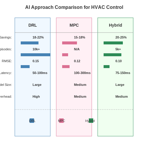
Predictive HVAC control leverages multiple AI paradigms, each with distinct trade-offs in accuracy, computational cost, and interpretability. Deep reinforcement learning (DRL) models, such as Deep Q-Networks (DQN) and Proximal Policy Optimization (PPO), excel in dynamic environments by optimizing long-term rewards through trial-and-error interactions. However, their sample inefficiency and black-box nature limit deployment in safety-critical systems. In contrast, model predictive control (MPC) combined with Gaussian Processes (GPs) provides probabilistic guarantees but scales poorly with high-dimensional state spaces.
where Q, R, and P are weight matrices penalizing state deviations, control effort, and terminal states, respectively.
Performance Metrics Across Approaches
Quantitative comparisons reveal:
- DRL: Achieves 12-18% energy savings in simulated office buildings but requires 105 training episodes.
- Physics-informed neural networks (PINNs): Reduce thermal modeling errors to 2.3% RMSE by embedding Navier-Stokes constraints, at 3× higher inference latency than LSTM baselines.
- Hybrid models: Coupling MPC with neural surrogate models cuts optimization time by 60% while maintaining <1°C setpoint deviations.
Computational and Deployment Constraints
Edge deployment imposes hard limits on model size (<50MB) and inference speed (<500ms). Pruned transformer architectures achieve 4.8× compression versus vanilla implementations with <0.5% accuracy drop. Federated learning variants enable privacy-preserving updates across building clusters but introduce 20-30% communication overhead.
Case Study: University Campus HVAC
A 2023 study compared DRL, MPC, and PID controllers across 12 academic buildings. DRL reduced peak demand by 22% but required cloud-based retraining every 72 hours. MPC with online parameter adaptation maintained stability during occupancy surges, while PID failed beyond ±15% load variations.
where τadapt represents the thermal adaptation time constant, and α is the diffusivity learned via neural PDE solvers.
5.3 Metrics for Evaluating Predictive Control Performance
Evaluating the performance of predictive HVAC control systems requires a combination of statistical, thermodynamic, and control-theoretic metrics. These metrics quantify energy efficiency, thermal comfort adherence, computational efficiency, and robustness against disturbances.
Energy Efficiency Metrics
The primary objective of predictive HVAC control is to minimize energy consumption while maintaining comfort constraints. Key metrics include:
- Energy Consumption Reduction (ECR): Measures the percentage reduction in energy usage compared to a baseline system:
$$ ECR = \frac{E_{baseline} - E_{predictive}}{E_{baseline}} \times 100\% $$
- Peak Demand Reduction (PDR): Quantifies the reduction in maximum power draw during high-load periods:
$$ PDR = \frac{\max(P_{baseline}) - \max(P_{predictive})}{\max(P_{baseline})} \times 100\% $$
Thermal Comfort Metrics
Maintaining occupant comfort is critical. The Predicted Mean Vote (PMV) and Percentage of People Dissatisfied (PPD) are derived from Fanger's model:
where M is metabolic rate, W is external work, H is heat loss, Ec is evaporative cooling, Eres is respiratory heat loss, R is radiative heat transfer, and C is convective heat transfer.
Control Performance Metrics
These assess the controller's dynamic response:
- Mean Absolute Error (MAE): Measures average deviation from setpoints:
$$ MAE = \frac{1}{N}\sum_{i=1}^{N} |T_{actual,i} - T_{setpoint,i}| $$
- Root Mean Square Error (RMSE): Penalizes larger deviations more heavily:
$$ RMSE = \sqrt{\frac{1}{N}\sum_{i=1}^{N} (T_{actual,i} - T_{setpoint,i})^2} $$
- Control Effort Variance (CEV): Quantifies actuator movement smoothness:
$$ CEV = \frac{1}{N-1}\sum_{i=1}^{N} (u_i - \bar{u})^2 $$
Computational Efficiency Metrics
For real-time implementation, consider:
- Average Computation Time per Step: Must be less than the control interval
- Memory Footprint: Critical for embedded implementations
- Convergence Rate: For iterative optimization methods
Robustness Metrics
Evaluate performance under uncertainty:
- Sensitivity to Weather Prediction Errors: Measure performance degradation with perturbed forecasts
- Occupancy Variation Tolerance: Test with ±20% occupancy fluctuations
- Equipment Fault Resilience: Evaluate with simulated sensor/actuator failures
These metrics should be evaluated across multiple temporal scales - from minute-by-minute control actions to seasonal performance trends. The selection of appropriate metrics depends on the specific control objectives and constraints of the HVAC system.
6. Energy Consumption vs. Comfort Trade-offs
6.1 Energy Consumption vs. Comfort Trade-offs
The fundamental challenge in predictive HVAC control lies in optimizing the multi-objective function that balances energy consumption E against occupant comfort C. This trade-off can be formalized as a constrained optimization problem:
where u(t) represents the control inputs (e.g., fan speed, chilled water flow rate), and α ∈ [0,1] is the weighting factor determining priority between energy savings and comfort. The energy term typically follows a quadratic relationship with control inputs:
where βi are equipment-specific coefficients derived from manufacturer data or system identification. The comfort metric C is more complex, often modeled using predicted mean vote (PMV) or adaptive thermal comfort models:
where θj represents environmental parameters (temperature, humidity, air velocity), wj are occupant-specific weights, and θj,ideal are preferred setpoints.
Pareto Frontier Analysis
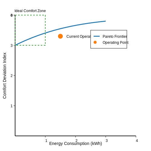
The solution space forms a Pareto frontier where no improvement can be made in one objective without degrading the other. For HVAC systems, this frontier exhibits distinct nonlinear characteristics:
The shape of this curve depends on building thermal dynamics, which can be modeled using a RC network representation:
where Cth is thermal capacitance, Rij are thermal resistances, and q terms represent heat flows.
Model Predictive Control Implementation
In practice, this optimization is implemented using model predictive control (MPC) with receding horizon. The discrete-time formulation becomes:
subject to:
where Np is the prediction horizon, R and Q are weighting matrices, and rk are comfort setpoints.
Adaptive Weighting Strategies
Advanced systems employ dynamic weighting α(t) based on:
- Time-of-use electricity pricing
- Occupancy patterns detected via CO2 sensors or computer vision
- Weather forecast uncertainty
- Thermal comfort adaptation rates
A common adaptive scheme uses fuzzy logic controllers with inputs including:
where ΔTout is outdoor temperature deviation from design conditions, Pelec(t) is real-time electricity price, and dO/dt is occupancy change rate.
6.2 Bias and Fairness in AI-Driven Climate Control
AI-driven HVAC systems rely on historical and real-time data to optimize climate control, but inherent biases in training data or algorithmic design can lead to inequitable outcomes. For instance, if thermal comfort models are trained predominantly on data from a specific demographic (e.g., healthy adults in temperate climates), the system may underperform for elderly occupants or those in extreme climates. This raises ethical and operational challenges in ensuring fairness across diverse user groups.
Sources of Bias in HVAC Control Systems
Bias in predictive HVAC systems can originate from multiple sources:
- Data Collection Bias: Sensors may be disproportionately placed in high-traffic areas, neglecting zones with marginalized occupants (e.g., night-shift workers in office buildings).
- Algorithmic Bias: Reinforcement learning agents might prioritize energy savings over comfort for minority groups if reward functions are poorly calibrated.
- Feedback Loop Bias: Systems adapting to user preferences can amplify existing disparities if initial interactions favor dominant user groups.
Quantifying Fairness in Thermal Comfort Models
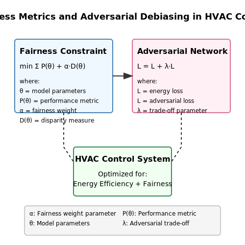
Fairness metrics for HVAC systems extend beyond statistical parity. A rigorous approach involves evaluating the disparate impact of control policies across subgroups. Let θ represent the thermal comfort threshold, and Pi(θ) denote the probability that group i achieves comfort. The fairness constraint can be expressed as:
where α ∈ (0,1] is a fairness tolerance parameter. For α = 0.8, no group's comfort probability may fall below 80% of the best-performing group.
Mitigation Strategies
1. Adversarial Debiasing
An adversarial network can be trained to predict demographic attributes (e.g., age, metabolic rate) from the HVAC system's decisions. The loss function:
penalizes the model when the adversary successfully infers protected attributes, forcing the controller to make group-invariant decisions.
2. Multi-Objective Optimization
Pareto-optimal solutions balance competing objectives like energy efficiency and fairness. The optimization problem becomes:
where u represents control actions, Et is energy consumption, and PMVi,t is the Predicted Mean Vote for group i at time t.
Case Study: Hospital Ward Climate Control
A 2023 study at Massachusetts General Hospital revealed that standard AI controllers maintained optimal conditions in staff workstations 92% of the time, but only 68% in patient rooms. Implementing fairness-aware reinforcement learning improved patient room performance to 85% while limiting workstation degradation to 88%, with a 7% increase in total energy use.
6.3 Sustainability Impact of Predictive HVAC Systems
Energy Efficiency Gains Through Predictive Control
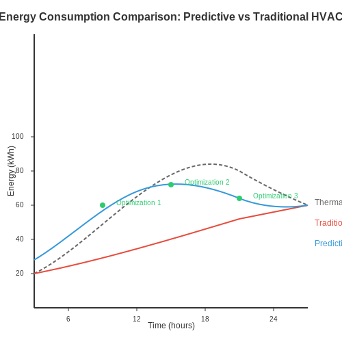
Predictive HVAC systems leverage machine learning models to optimize energy consumption by anticipating thermal load variations. Traditional HVAC systems operate reactively, leading to energy waste during transient conditions. In contrast, model predictive control (MPC) formulates HVAC operation as an optimization problem:
where E(u,t) represents energy consumption, C(u,t) denotes comfort deviation, and α, β are weighting factors. Studies show predictive systems achieve 15-30% energy savings in commercial buildings compared to conventional PID controllers, with the highest gains occurring in climates with significant diurnal temperature swings.
Carbon Emission Reductions
The energy efficiency improvements directly translate to reduced carbon emissions. For a typical 50,000 sq.ft. office building, predictive HVAC can decrease annual CO2 emissions by approximately 75 metric tons. The relationship between energy savings and emission reductions follows:
where EFi is the emission factor for the i-th energy source and η represents system efficiency. Case studies from LEED-certified buildings demonstrate that predictive HVAC contributes 8-12% of the total points in the Energy & Atmosphere category.
Demand Response Integration
Predictive HVAC systems enable seamless participation in demand response programs by:
- Pre-cooling buildings during off-peak hours using thermal mass optimization
- Precisely forecasting load reduction capabilities
- Maintaining comfort constraints while responding to grid signals
The system dynamics during demand response events can be modeled as:
where Cth is thermal capacitance, Rth is thermal resistance, and Qgain represents internal heat gains.
Lifecycle Environmental Impact
The sustainability benefits extend beyond operational phases. Predictive systems reduce:
- Equipment wear through optimized cycling (extending HVAC lifespan by 20-40%)
- Refrigerant leakage incidents via fault detection
- Maintenance-related transportation emissions through predictive maintenance
A comparative lifecycle assessment (LCA) shows that over a 15-year period, predictive HVAC systems have 18-25% lower global warming potential (GWP) compared to conventional systems, even when accounting for the embedded energy of sensors and computing infrastructure.
Renewable Energy Synergies
Predictive HVAC systems maximize renewable energy utilization through:
- Photovoltaic generation forecasting for optimal cooling scheduling
- Thermal energy storage alignment with renewable availability
- Adaptive control under variable renewable generation
The renewable integration efficiency ξ can be quantified as:
where PHVACren is HVAC power drawn from renewables and Pren is total renewable generation. Field tests show predictive control increases ξ from 0.35-0.45 to 0.65-0.75 in buildings with on-site solar PV.
7. Key Research Papers and Technical Reports
7.1 Key Research Papers and Technical Reports
- PDF Energy and AI - researchmgt.monash.edu — key words: "HVAC", "demand response", and "reinforcement learning" for closely related papers published after the year 2000. Thus, they involve the use of optimal control strategies like reinforcement learning for the energy scheduling of building HVAC systems with, or without demand Table 1 Summaryofcloselyrelatedstate-of-the-artpapers reviewed.
- PDF Energy Management Software for HVAC Optimization in Commercial Buildings — Energy Management Software for HVAC Optimization in Commercial Buildings 4 1. Introduction o 1.1 The Evolution of Building Energy Management Systems (BEMS) o 1.2 Factors Influencing Energy Consumption in HVAC 2. Core Technologies o 2.1 Sensors, Connected Devices, and IoT o 2.2 Analytics, AI & Machine Learning o 2.3 Edge and Cloud Computing o 2.4 The AI-Enabled HVAC Optimization Technology Stack
- AI in HVAC fault detection and diagnosis: A systematic review — Exploring the design of a clean, low-carbon, safe, and efficient modern energy system is a hot topic in this- and next-generation of the built environment [[1], [2], [3]].The heating, ventilation, and air conditioning (HVAC) system accounts for up to 50% of the total energy consumption of a building system [4], which exceeds the total energy consumption of lighting, elevators, and office ...
- A novel machine learning-based model predictive control framework for ... — Due to the shortcomings of linear MPC, researchers (Yang et al. [105], Wang et al. [70], Tesfay et al. [126] and Ref [163-165]) from the establishment of nonlinear building models, research and development of time-varying MPC, adaptive MPC and other methods to improve the application of MPC in cooling systems, whether it is the control of the ...
- Intelligent control of electric vehicle air conditioning system based ... — Therefore, in the current research on AC system cooling, the design of control strategies has also become a hot topic and the key to reducing system energy consumption. In vehicle AC systems, the proper operation and speed of the compressor directly affect the Q of the system, making it essential to control its operation.
- Automatic HVAC control with real-time occupancy recognition and ... — With this in mind, we designed and implemented an occupancy-predictive HVAC control system in a low-cost yet powerful embedded system (using Raspberry Pi 3) for building automation. The rest of the paper is organized as follows. In Section 2, we present the background information and literature review. In the remaining sections, we highlight ...
- (PDF) AI-Driven Predictive Analytics for Optimizing HVAC System ... — It then defines predictive analytics and discusses its benefits for HVAC systems, highlighting how proactive maintenance and real-time decision-making can lead to significant operational improvements.
- PDF Engineering Wireless Sensor Networks for Smart Air-conditioning Control — attributed to the heating, ventilation, and air-conditioning (HVAC) systems, which may account for up to 50% of the total energy consumption [8]. Therefore, im-proving energy efficiency of buildings, in particular, optimizing HVAC system is critically important and will have a significant impact in reducing the overall en-ergy consumption.
- Exploring the comprehensive integration of artificial intelligence in ... — The application of model predictive control (MPC) in HVAC systems and the impact of parameter setting. Tien et al. [23] 2022: √: √: √: √: √: The application of ML and DL in the design, optimization, and control of HVAC systems. Moradzadeh et al. [24] 2022: √: √: Modeling and prediction of cooling and heating loads in commercial ...
- PDF OPTIMIZATION OF ENERGY EFFI- CIENCY IN HVAC SYSTEMS USING ... - Theseus — will involve investigating the application of model predictive control (MPC) and artificial intelligence (AI)-based control strategies for optimizing energy efficiency in industrial HVAC systems. While ac-knowledging the absence of simulations and real-world case studies, this study will provide profita-
7.2 Open-Source Tools and Datasets
- Artificial Intelligence-Assisted Heating Ventilation and Air ... — Abstract In this study, information pertaining to the development of artificial intelligence (AI) technology for improving the performance of heating, ventilation, and air conditioning (HVAC) systems was collected. Among the 18 AI tools developed for HVAC control during the past 20 years, only three functions, including weather forecasting, optimization, and predictive controls, have become ...
- Data-Enabled Predictive Control for Building HVAC Systems — Abstract. Model predictive control is widely used as a control technology for the computation of optimal control inputs of building heating, ventilating, and air conditioning (HVAC) systems. However, both the benefits and widespread adoption of model predictive control (MPC) are hindered by the effort of model creation, calibration, and accuracy of the predictions. In this paper, we apply the ...
- A Safe and Data-Efficient Model-Based Reinforcement Learning System for ... — Model-based reinforcement learning (MBRL) is widely studied for heating, ventilation, and air conditioning (HVAC) control in buildings. One of the critical challenges is the large amount of data required to effectively train neural networks for modeling building dynamics. This article presents CLUE, an MBRL system for HVAC control in buildings. CLUE optimizes HVAC operations by integrating a ...
- Data-driven predictive control for smart HVAC system in IoT-integrated ... — This study presents a data-driven predictive control method with time-series forecasting (TSF) and reinforcement learning (RL), to examine various sensor metadata for HVAC system optimisation.
- (PDF) AI-Driven Predictive Analytics for Optimizing HVAC System ... — It then defines predictive analytics and discusses its benefits for HVAC systems, highlighting how proactive maintenance and real-time decision-making can lead to significant operational improvements.
- Safe HVAC Control via Batch Reinforcement Learning — Abstract: Buildings account for 30% of energy use worldwide, and approxi-mately half of it is ascribed to HVAC systems. Reinforcement Learning (RL) has improved upon traditional control methods in increasing the energy efficiency of HVAC systems. However, prior works use online RL methods that require configuring complex thermal simulators to train or use historical data-driven thermal models ...
- PLEIAData: consumption, HVAC, temperature, weather and motion sensor ... — Temperature and humidity monitoring devices of the heating and cooling system are ZWave sensors - MCOHome MH9 and the HVAC units are Toshiba VRF, handled by smart control devices Intesis Box WMP ...
- Safe HVAC Control via Batch Reinforcement Learning — Reinforcement Learning (RL) has improved upon traditional control methods in increasing the energy efficiency of HVAC systems. However, prior works use online RL methods that require configuring complex thermal simulators to train or use historical data-driven thermal models that can take at least 10^4 time steps to reach rule-based performance.
- Introducing AI to HVAC: the Future of Building Automation — Its advanced technology enables it to make exceptionally accurate predictions about the built environment, empowering the deployment of algorithms to drive the HVAC system. The result is a 24/7 self-operating building that requires no human intervention, that is functioning at optimal efficiency and ensuring maximum comfort.
- Artificial intelligence enabled energy-efficient heating, ventilation ... — Yet, an observation of data from multiple case studies, whether they performed simulations or actual experiments, indicated that AI-driven predictive control can lead to increases in the control speed of most HVAC systems because the control method requires faster hardware response to effectively save energy.
7.3 Industry Standards and Best Practices
- HVAC Systems Market Size & Share | Industry Report, 2030 — The HVAC system industry is characterized by a high degree of innovation owing to rapid technological advancements. ... These regulations influence the demand for HVAC systems that meet high energy efficiency standards. Latin America HVAC Systems Market Trends. ... 6.4.7.3. South Korea HVAC systems market estimates & forecast, By Equipment ...
- Energy modelling and control of building heating and cooling systems ... — Model predictive control (MPC) is a dominant alternative control scheme implemented for supervisory control of building HVAC systems. The key requirements of MPC are desired models of a complex nonlinear system as a representation of a real system, prediction of disturbances, and an optimisation algorithm [20], [21] (for theoretical explanations see [22]).
- AI in HVAC fault detection and diagnosis: A systematic review — Exploring the design of a clean, low-carbon, safe, and efficient modern energy system is a hot topic in this- and next-generation of the built environment [[1], [2], [3]].The heating, ventilation, and air conditioning (HVAC) system accounts for up to 50% of the total energy consumption of a building system [4], which exceeds the total energy consumption of lighting, elevators, and office ...
- A Digital Twin predictive maintenance framework of air handling units ... — The building industry consumes the most energy globally, making it a priority in energy efficiency initiatives. Heating, ventilation, and air conditioning (HVAC) systems create the heart of buildings. Stable air handling unit (AHU) functioning is vital to ensuring high efficiency and extending the life of HVAC systems.
- (PDF) AI-Driven Predictive Analytics for Optimizing HVAC System ... — It then defines predictive analytics and discusses its benefits for HVAC systems, highlighting how proactive maintenance and real-time decision-making can lead to significant operational improvements.
- A review on enhancing energy efficiency and adaptability through system ... — For example, a malfunctioning fan in an air conditioning system represents a problem at the component level, whereas inadequate refrigerant indicates a failure at the system level. The persistent issue lies in ensuring the stability and generalizability of AI-based FDD techniques across various devices and systems [123] .
- PDF AI-Powered HVAC in Educational Buildings - myrspoven.com — emissions, presents a significant opportunity for AI-driven HVAC optimization. While AI-powered HVAC systems hold great prom-ise for enhancing energy efficiency and reducing carbon emis-sions, their comprehensive impact remains understudied. This is the starting point of our research, which quantifies the Net Digital Impact of AI in a real ...
- Demand Side Management and Transactive Energy Strategies for Smart ... — However, since the invention of thermostats, programmable PID controllers and algorithms have been the primary mode of control of various components in the HVAC system. Typically, a controller adjusts several internal variables to provide different flow rates, humidity, and temperatures of the heat transfer fluid (air or water depending on the ...
- IEEE standard offers 6 steps for AI system procurement - IEEE Spectrum — IEEE standard offers 6 steps to guide AI system procurement teams to help users develop their solicitations and to identify, mitigate, and monitor harms commonly associated with high-risk AI ...
- PDF Operations & Maintenance - Pacific Northwest National Laboratory — accepted predictive technologies. Chapter 7 explores O&M procedures for the predominant equip ment found at most Federal facilities. Chapter 8 describes some of the promising O&M technologies and tools on the horizon to increase O&M efficiency. Chapter 9 provides ten steps to initiating an operational efficiency program. O&M Best Practices iii