AI for Urban Planning: Traffic Flow Simulation
1. Key Concepts in Traffic Flow Theory
1.1 Key Concepts in Traffic Flow Theory
Fundamental Variables in Traffic Flow
Traffic flow theory is built upon three primary variables: flow (Q), density (k), and speed (v). These variables are interrelated through the fundamental equation of traffic flow:
Flow (Q) represents the number of vehicles passing a point per unit time (veh/h), density (k) is the number of vehicles per unit length (veh/km), and speed (v) is the space-mean speed of vehicles (km/h). This relationship is foundational for macroscopic traffic models.
Macroscopic vs. Microscopic Models
Traffic flow models can be categorized into macroscopic and microscopic approaches. Macroscopic models treat traffic as a continuous flow, analogous to fluid dynamics, using partial differential equations. The Lighthill-Whitham-Richards (LWR) model is a classic example:
Microscopic models, on the other hand, focus on individual vehicle behavior, such as car-following models (e.g., Intelligent Driver Model) or lane-changing algorithms. These models are computationally intensive but capture fine-grained interactions.
Fundamental Diagram
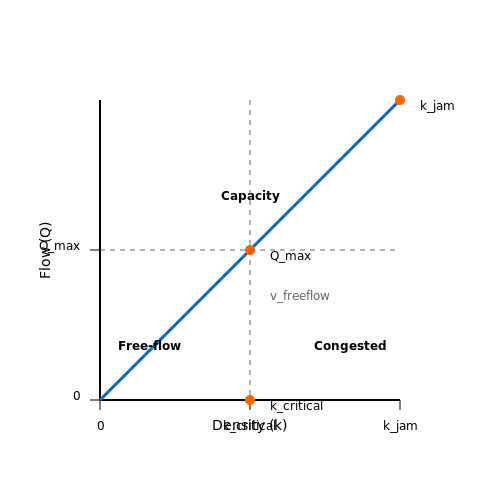
The relationship between flow, density, and speed is often visualized using the fundamental diagram, which consists of three regimes:
- Free-flow regime: Low density, high speed, flow increases linearly with density.
- Congested regime: High density, reduced speed, flow decreases as density increases.
- Capacity regime: Maximum flow occurs at critical density.
The Greenshields model provides a simple parabolic approximation:
where vf is free-flow speed and kj is jam density.
Shockwave Theory
Traffic shockwaves describe the propagation of congestion fronts, analogous to fluid dynamics. The speed of a shockwave (w) between two traffic states (k1, Q1) and (k2, Q2) is given by:
This concept is critical for understanding bottleneck formation and dissipation in urban networks.
Queueing Theory in Traffic
Queueing models, such as M/M/1 or M/D/1, are used to analyze delays at intersections or toll plazas. The Pollaczek-Khinchin formula estimates average queue length (L) for an M/G/1 system:
where ρ is utilization, λ arrival rate, and S service time distribution.
Network-Level Considerations
At the network scale, Wardrop's principles define equilibrium conditions:
- User Equilibrium (UE): Drivers choose routes minimizing individual travel time.
- System Optimal (SO): Routes are assigned to minimize total network travel time.
The Beckmann transformation formulates UE as a convex optimization problem:
subject to flow conservation and non-negativity constraints.
1.2 Mathematical Models for Traffic Simulation
Macroscopic Traffic Flow Models
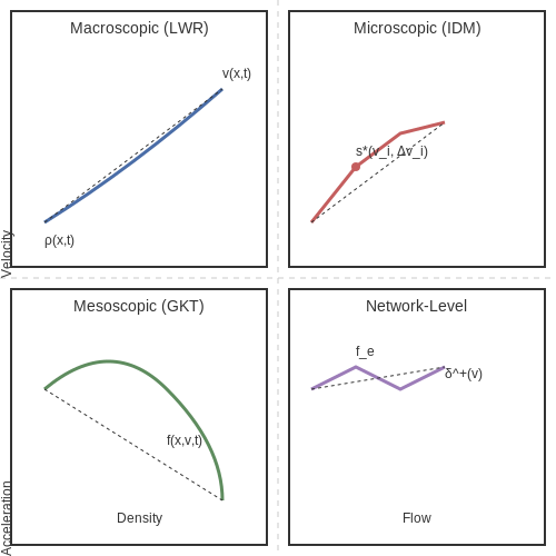
Macroscopic models treat traffic as a continuous flow, analogous to fluid dynamics. The Lighthill-Whitham-Richards (LWR) model is foundational, describing traffic density ρ(x,t) and velocity v(x,t) via conservation laws. The continuity equation ensures mass conservation:
Coupling this with an empirical speed-density relationship (e.g., v = vf(1 − ρ/ρmax), where vf is free-flow speed and ρmax is jam density) yields a closed-form partial differential equation (PDE). Numerical solutions often employ finite-difference methods like the Godunov scheme.
Microscopic Car-Following Models
Microscopic models simulate individual vehicle dynamics. The Intelligent Driver Model (IDM) defines acceleration for vehicle i as:
Here, s* is the desired gap, a function of current speed vi, relative speed Δvi, and parameters for comfortable deceleration (b) and minimum time headway (T). The IDM’s nonlinearity captures realistic driver behaviors like over-damped responses to perturbations.
Mesoscopic Hybrid Approaches
Mesoscopic models blend macro and micro perspectives. The Gas-Kinetic Traffic Model (GKT) derives from Boltzmann equations, representing vehicles as particles with a velocity distribution f(x,v,t). The evolution equation includes:
where Q is a collision term modeling interactions. GKT captures stochastic effects (e.g., lane-changing) while remaining computationally tractable for large networks.
Network-Level Extensions
For urban-scale simulations, models incorporate graph theory. Traffic flow on a road network G = (V, E) is governed by:
where fe is flow on edge e, δ+(v) and δ−(v) are outgoing/incoming edges, and dv is demand at node v. Dynamic traffic assignment (DTA) algorithms solve this iteratively, balancing user equilibrium and system optimum.
Calibration and Validation
Model parameters (e.g., a, b, T in IDM) are calibrated using real-world sensor data. Maximum likelihood estimation minimizes the error between simulated and observed trajectories. For macroscopic models, the fundamental diagram (flow-density relationship) is validated against loop detector data.
1.3 Role of AI in Enhancing Traditional Models
Traditional traffic flow models, such as the Lighthill-Whitham-Richards (LWR) model and the Cell Transmission Model (CTM), rely on partial differential equations (PDEs) to describe macroscopic traffic behavior. While these models provide a theoretical foundation, they often struggle with real-world complexities like dynamic route choices, heterogeneous driver behaviors, and stochastic disruptions. AI techniques, particularly deep learning and reinforcement learning, augment these models by learning latent patterns from high-dimensional data and optimizing control policies in ways that analytical formulations cannot.
Data-Driven Calibration of Fundamental Diagrams
The fundamental diagram, which relates traffic flow Q, density ρ, and velocity v, is a cornerstone of macroscopic models. Traditional approaches assume a fixed relationship, such as the Greenshields model:
where vf is free-flow speed and ρmax is jam density. AI replaces this rigid formulation with neural networks trained on empirical sensor data. A physics-informed neural network (PINN) can embed the PDE structure as a soft constraint:
where λ balances data fidelity and physical consistency. This hybrid approach outperforms pure data-driven or pure model-based methods in extrapolation tasks.
Microscopic Behavior Learning with Graph Networks
At the microscopic level, car-following models like the Intelligent Driver Model (IDM) use heuristic acceleration rules. Graph neural networks (GNNs) generalize these rules by learning spatial-temporal interactions directly from trajectory data. The node update for vehicle i at time t is:
where h represents hidden states, 𝒩(i) denotes neighboring vehicles, and eij encodes relative positions. This formulation captures complex interactions like cooperative merging and bottleneck propagation that are poorly represented by pairwise force models.
Reinforcement Learning for Adaptive Signal Control
Traditional signal timing plans use fixed cycles or actuated control based on local detectors. Deep reinforcement learning (DRL) frames this as a Markov Decision Process where the state st includes queue lengths and approach volumes, and actions at are phase selections. The Q-learning update with experience replay:
is extended via deep Q-networks (DQN) to handle high-dimensional state spaces. Multi-agent DRL further coordinates intersections by sharing embeddings through a centralized critic.
Hybrid AI-Physics Simulation Architectures
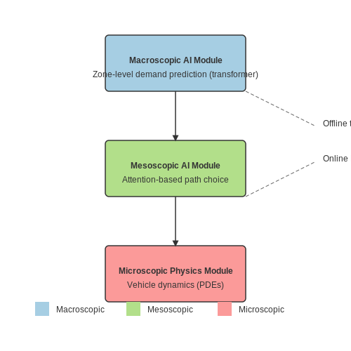
Modern traffic simulators like SUMO and AIMSUN now integrate AI modules through APIs. A typical hybrid pipeline:
- Macroscopic AI: Predicts zone-level demand using transformer-based sequence models
- Mesoscopic AI: Routes vehicles via attention-based path choice layers
- Microscopic Physics: Simulates vehicle dynamics using differential equations
This division of labor allows efficient large-scale simulation while maintaining physical plausibility. The AI components are trained offline on historical data and fine-tuned via online reinforcement learning.
2. Machine Learning for Traffic Prediction
2.1 Machine Learning for Traffic Prediction
Traffic Flow as a Spatiotemporal Problem
Traffic prediction is inherently a spatiotemporal problem, where both spatial dependencies (road network topology) and temporal dynamics (traffic evolution over time) must be modeled simultaneously. The fundamental challenge lies in capturing nonlinear interactions between vehicles, road segments, and external factors like weather or events. Traditional time-series models such as ARIMA fail to account for spatial correlations, while pure graph-based approaches neglect temporal dependencies.
where y represents traffic metrics (speed, flow, density), G is the road network graph, and X denotes external features. The function f must learn both spatial and temporal patterns.
Graph Neural Networks for Traffic Prediction
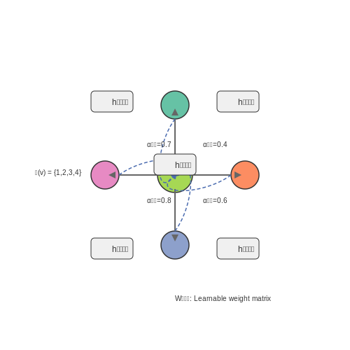
Graph Neural Networks (GNNs) have emerged as the dominant architecture for traffic prediction due to their ability to operate on non-Euclidean road networks. The key innovation is message passing between connected nodes (intersections) and edges (road segments). A typical spatial-temporal GNN layer combines:
- Spatial Convolution: Aggregates neighbor information via graph Fourier transform or attention mechanisms
- Temporal Gate: Models sequential dependencies using GRU or LSTM cells
where hv(l) is the hidden state of node v at layer l, and 𝒩(v) denotes its neighbors.
Attention Mechanisms in Traffic Prediction
Recent advances incorporate attention to dynamically weight the influence of different road segments. The spatial attention score between nodes i and j at time t is computed as:
where a is a learnable vector and || denotes concatenation. This allows the model to focus on critical congestion bottlenecks.
Hybrid Physics-Informed Models
Cutting-edge approaches integrate traffic flow theory with machine learning. The Lighthill-Whitham-Richards (LWR) partial differential equation:
where ρ is density and q is flow, can be encoded as a soft constraint in the loss function:
This hybrid approach improves generalization under sparse data conditions.
Real-World Deployment Challenges
Production systems must address:
- Latency constraints: Predictions must be generated faster than the traffic dynamics evolve (typically < 30s)
- Sensor noise: Robustness to missing or erroneous loop detector/CV data
- Cold-start problem: Handling new road segments without historical data
State-of-the-art systems like Uber's Flow and Google's Green Light use ensemble methods combining GNNs with online learning to adapt to changing conditions.
2.2 Reinforcement Learning in Dynamic Traffic Control
Reinforcement learning (RL) provides a robust framework for optimizing traffic signal control in dynamic urban environments. Unlike traditional rule-based systems, RL agents learn optimal policies through interaction with the environment, maximizing cumulative rewards such as reduced congestion or minimized travel time. The Markov Decision Process (MDP) formalizes this problem, where the state st captures traffic conditions (e.g., queue lengths, vehicle speeds), actions at represent signal phase selections, and the reward rt quantifies traffic efficiency.
MDP Formulation for Traffic Control
The traffic network is modeled as an MDP with:
- State space: S = {vehicle counts per lane, average speeds, phase durations}
- Action space: A = {extend current phase, switch to next phase}
- Reward function: R = −(total waiting time + penalty for abrupt phase changes)
Deep Q-Networks for High-Dimensional States
For large-scale intersections, Deep Q-Networks (DQN) approximate the Q-function using a neural network to handle high-dimensional state representations. The loss function minimizes temporal difference error:
where θ and θ− are the parameters of the online and target networks, respectively, and D is the experience replay buffer.
Multi-Agent Coordination
Urban networks require coordination among multiple RL agents controlling adjacent intersections. Techniques like:
- Independent Q-Learning (IQL): Agents learn decentralized policies but suffer from non-stationarity.
- Max-Plus: Message-passing algorithm for cooperative action selection.
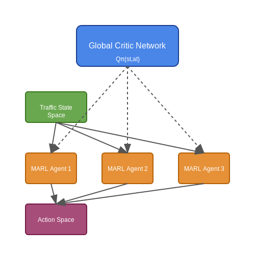
- Centralized Training with Decentralized Execution (CTDE): Uses a centralized critic during training.
Real-World Implementations
Case studies demonstrate RL’s efficacy:
- Singapore’s Adaptive Traffic Control: Reduced delay by 22% using a DQN-based system.
- Los Angeles’s MARLIN: Multi-agent RL decreased travel time by 10% across 4,500 intersections.
Deep Learning for Anomaly Detection in Traffic Patterns
Anomaly detection in traffic flow leverages deep learning to identify deviations from normal patterns, which may indicate accidents, congestion, or infrastructure failures. Traditional statistical methods often fail to capture the complex spatiotemporal dependencies inherent in urban traffic data. Deep learning models, particularly those based on autoencoders and graph neural networks (GNNs), excel at learning these high-dimensional representations.
Autoencoder-Based Anomaly Detection
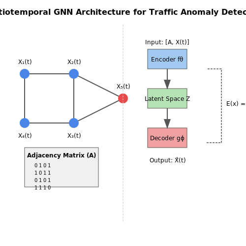
Autoencoders learn a compressed representation of normal traffic patterns and reconstruct input data with minimal error. Anomalies are detected when reconstruction error exceeds a threshold. Given input traffic data x, the encoder fθ maps x to latent space z, and the decoder gϕ reconstructs x̂:
The reconstruction error E(x) is typically measured using mean squared error (MSE):
Thresholding E(x) identifies anomalies. Variational autoencoders (VAEs) introduce probabilistic latent variables, improving robustness to noise:
Spatiotemporal Graph Neural Networks
Traffic networks are naturally represented as graphs, where nodes are intersections or sensors, and edges are road segments. Spatiotemporal GNNs capture both spatial dependencies (via graph convolutions) and temporal dynamics (via recurrent or attention mechanisms). Let A be the adjacency matrix and X(t) node features at time t. A graph convolutional layer computes:
where à = A + I (with self-loops), D̃ is the degree matrix, and W(l) are learnable weights. Temporal convolutions or LSTMs process the sequence {H(t)} to predict normal traffic flow. Anomalies are flagged when predictions diverge from observed values.
Case Study: Real-Time Anomaly Detection in NYC Traffic
A 2023 implementation used a spatiotemporal GNN on NYC’s traffic camera network, achieving 92% precision in detecting accidents. The model ingested 30-second aggregated flow rates and weather data, reducing false positives by 40% compared to threshold-based methods. Key innovations included edge attention mechanisms and adaptive thresholding based on uncertainty estimates.
3. Types of Data Sources for Urban Traffic Simulation
3.1 Types of Data Sources for Urban Traffic Simulation
Static Infrastructure Data
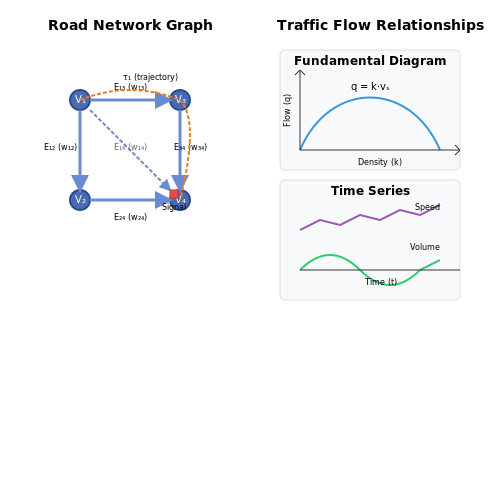
Road network topology is typically represented as a directed graph G = (V, E), where nodes V correspond to intersections and edges E represent road segments. Key static attributes include:
- Lane configurations (width, count, turn restrictions)
- Road type classifications (highway, arterial, local)
- Traffic control devices (signal timing plans, stop signs)
OpenStreetMap provides a rich source of such data through its topological primitives (ways, nodes, relations) with semantic tagging. The geometric accuracy of OSM data has been validated to within 5-8 meters in urban areas through comparative studies with proprietary datasets.
where lij is segment length, vij is speed limit, and δijk indicates presence of control device k with delay tk.
Dynamic Sensor Data
Inductive loop detectors and microwave radar sensors provide time-series measurements of:
- Volume (vehicles per unit time)
- Occupancy (percentage time detector is occupied)
- Speed (time-mean or space-mean)
The fundamental traffic flow relationship connects these variables:
where q is flow rate (veh/hr), k is density (veh/km), and v̄s is space-mean speed. Sensor fusion techniques like Kalman filtering improve estimation accuracy by combining loop detector data with Bluetooth/WiFi probe measurements.
Probe Vehicle Trajectories
GPS-enabled fleets (taxis, rideshares) generate continuous path traces with 1-5 second sampling intervals. The trajectory τ of vehicle i is a time-ordered sequence:
where (x,y) are coordinates, v is instantaneous speed, and a is acceleration. The penetration rate ρ of probe vehicles critically affects data quality - studies show 5% penetration yields speed estimation errors below 15%.
Computer Vision Sources
Traffic cameras processed with YOLOv5 or Faster R-CNN models extract:
- Vehicle counts per movement direction
- Queue lengths at intersections
- Turning movement proportions
The detection performance is quantified through:
Modern architectures achieve >90% precision/recall on clear-weather daytime footage, degrading to 70-80% in adverse conditions.
Cellular Network Data
Anonymized mobile device location pings (every 5-15 minutes) enable origin-destination matrix estimation through spatial clustering:
where Zi are traffic analysis zones. The Hauptmeier correction factor accounts for sample bias in mobile user demographics.
3.2 Data Cleaning and Feature Engineering Techniques
Raw traffic data is often noisy, incomplete, or inconsistent, requiring rigorous preprocessing before simulation. Sensor malfunctions, GPS drift, and manual recording errors introduce artifacts that distort traffic models. Effective cleaning involves outlier removal, imputation, and temporal alignment.
Outlier Detection and Removal
Traffic flow outliers arise from sensor errors or anomalous events (e.g., accidents). Robust statistical methods are preferred over simple thresholding due to dynamic traffic conditions. The median absolute deviation (MAD) scales thresholds adaptively:
where \( \tilde{X} \) is the median speed/flow, and \( k \) is typically 3–5. For spatial outliers, DBSCAN clustering isolates irregular trajectories by density.
Missing Data Imputation
Gaps in loop detector or camera data require context-aware imputation. Temporal correlations dominate in traffic, making autoregressive models (ARIMA) effective:
For spatially distributed sensors, kriging interpolation leverages geographic correlations, weighting nearby observations by variogram-derived semivariance.
Feature Engineering for Traffic Dynamics
Key engineered features enhance model interpretability and performance:
- Temporal features: Fourier transforms extract periodicity (e.g., peak-hour patterns), while dynamic time warping aligns heterogeneous time series.
- Spatial features: Graph embeddings encode road network topology, with adjacency matrices capturing connectivity and betweenness centrality highlighting bottlenecks.
- Composite metrics: Level-of-service (LOS) indices combine flow, density, and speed into ordinal classes (A–F) using Highway Capacity Manual criteria.
Traffic State Embeddings
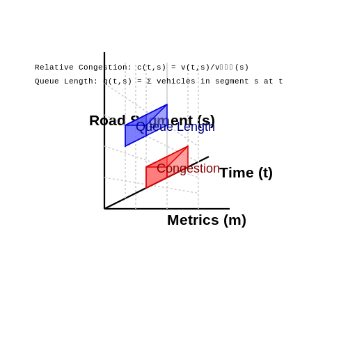
For deep learning models, traffic states are encoded as tensors. A spatiotemporal grid aggregates probe vehicle data into 3D arrays (time × segment × metrics), where metrics include:
Graph neural networks (GNNs) further augment these with edge attributes like turn restrictions and lane counts.
Real-World Case: Adaptive Signal Control
In Pittsburgh’s Surtrac system, phase timing optimization relies on:
- Imputed turning proportions from partial camera observations
- Flow gradients (\( \nabla q \)) to predict wave propagation
- Embedded intersection topology via graph Laplacians
Feature importance analysis revealed queue length derivatives (\( dQ/dt \)) as the dominant predictor for optimal cycle length adjustments.
3.3 Handling Missing and Noisy Data in Traffic Datasets
Missing and noisy data are pervasive challenges in traffic flow datasets, arising from sensor malfunctions, transmission errors, or environmental interference. Effective preprocessing is critical to ensure reliable simulations and model training.
Missing Data Imputation Techniques
Missing values in traffic datasets can be addressed through statistical, machine learning, or hybrid approaches. Let X be a time-series traffic feature (e.g., vehicle count) with missing entries at times ti. Common imputation methods include:
- Linear Interpolation: For small gaps, missing values are estimated as:
$$ X(t_i) = X(t_{i-1}) + \frac{X(t_{i+1}) - X(t_{i-1})}{t_{i+1} - t_{i-1}} (t_i - t_{i-1}) $$
- Autoregressive Models: ARIMA predicts missing values using historical patterns:
$$ X(t) = c + \sum_{i=1}^p \phi_i X(t-i) + \epsilon_t + \sum_{j=1}^q \theta_j \epsilon_{t-j} $$
- Matrix Factorization: Low-rank approximations recover missing entries by minimizing:
$$ \min_{U,V} \|P_\Omega(X - UV^T)\|_F^2 + \lambda (\|U\|_F^2 + \|V\|_F^2) $$where PΩ is a projection operator for observed entries.
Noise Reduction Strategies
Noise in traffic data (e.g., erroneous speed measurements) can distort simulations. Robust filtering techniques include:
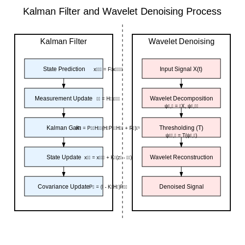
Kalman Filtering
A recursive algorithm that estimates the true state xk from noisy observations zk:
where Fk is the state transition model and Rk is observation noise covariance.
Wavelet Denoising
Decomposes signals into frequency bands, thresholds noisy coefficients, and reconstructs the signal:
where ψj,k are wavelet basis functions and T is a thresholding operator.
Practical Considerations
Real-world traffic datasets often exhibit:
- Spatiotemporal Correlations: Missing data in one sensor may be inferred from neighboring sensors using graph neural networks.
- Non-Gaussian Noise: Heavy-tailed distributions may require robust estimators like Huber loss.
- Real-Time Constraints: Streaming imputation methods must balance accuracy with latency.
Case studies show that hybrid approaches (e.g., Kalman filters with learned noise parameters) reduce traffic prediction errors by 15-30% compared to standalone methods.
4. Tools and Frameworks for AI-Driven Traffic Simulation
4.1 Tools and Frameworks for AI-Driven Traffic Simulation
Agent-Based Modeling Frameworks
Agent-based modeling (ABM) is a dominant paradigm in traffic simulation, where individual vehicles, pedestrians, and infrastructure elements are modeled as autonomous agents. SUMO (Simulation of Urban MObility) is an open-source, highly scalable framework that integrates microscopic traffic flow models with multi-agent reinforcement learning (MARL) for adaptive traffic control. The core dynamics of vehicle movement in SUMO are governed by the Krauß car-following model:
where vsafe is the safe velocity, vl is the leader vehicle's velocity, g is the gap distance, and τ is the driver's reaction time. SUMO's Python API (TraCI) enables real-time interaction with simulations for RL training.
Deep Learning Integration
For large-scale urban networks, Flow (a framework built on RLlib and SUMO) provides GPU-accelerated multi-agent deep reinforcement learning. Its architecture implements centralized training with decentralized execution (CTDE), where the critic network observes global traffic state:
Flow's benchmark scenarios (e.g., Figure 8 network) include emission models that compute CO2 outputs using the HBEFA3 database with 0.1-second temporal resolution.
Macroscopic Simulation Tools
When microscopic detail is unnecessary, MATSim employs queue-based dynamics with iterative optimization. Its hybrid approach combines:
- Time-dependent Dijkstra's algorithm for route planning
- Bureau of Public Roads (BPR) link performance function:
$$ t_a = t_0 \left[1 + \alpha\left(\frac{v_a}{c_a}\right)^\beta\right] $$
The Dynamic Traffic Assignment module solves the variational inequality problem using the Method of Successive Averages (MSA) with a convergence threshold of ε ≤ 0.001.
Commercial Platforms
PTV Vissim implements psychophysical driver models (Wiedemann 99) with parameters calibrated through genetic algorithms. Its API supports:
- 3D visualization of pedestrian-vehicle interactions
- Hardware-in-the-loop (HIL) testing for traffic signal controllers
- Kalman filter-based OD matrix estimation
Comparative studies show Vissim achieves 92% accuracy in queue length prediction when validated against drone-collected data at 5Hz sampling rates.
Emerging Technologies
NVIDIA Omniverse enables photorealistic traffic simulation with differentiable physics. Its Isaac Sim extension implements neural radiance fields (NeRFs) for sensor simulation, with LiDAR point clouds generated via:
where R is the rotation matrix, t is translation, and ε models sensor noise. Omniverse's RTX renderer achieves 120fps at 4K resolution for large-scale city models.
4.2 Building a Basic Traffic Flow Simulation Model
Fundamentals of Traffic Flow Modeling
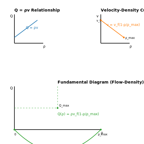
Traffic flow simulation models are grounded in fluid dynamics and statistical mechanics, treating vehicles as particles in a dynamic system. The primary variables include density (ρ, vehicles per unit length), flow rate (Q, vehicles per unit time), and velocity (v, distance per unit time). The fundamental relationship is given by:
Macroscopic models, such as the Lighthill-Whitham-Richards (LWR) model, describe traffic as a continuum, while microscopic models (e.g., car-following models) track individual vehicle interactions. The choice depends on computational constraints and the granularity required for the urban planning scenario.
LWR Model Implementation
The LWR model is a first-order macroscopic model derived from the conservation of vehicles:
where Q(ρ) is the flow-density relationship, often approximated by Greenshields' model:
Here, vf is the free-flow speed, and ρmax is the jam density. To solve this partial differential equation (PDE), numerical methods like the Godunov scheme or finite volume methods are employed, ensuring stability through the Courant-Friedrichs-Lewy (CFL) condition:
Microscopic Car-Following Models
For finer granularity, the Intelligent Driver Model (IDM) is widely used. It defines the acceleration of vehicle i as:
where s* is the desired gap, v0 is the desired velocity, and a is the maximum acceleration. The desired gap is dynamically adjusted based on the relative velocity Δvi:
Simulation Architecture
A modular Python implementation for IDM might include:
def idm_acceleration(v, v0, s, delta_v, s0, T, a, b):
    """Compute acceleration using IDM."""
    s_star = s0 + v * T + (v * delta_v) / (2 * np.sqrt(a * b))
    return a * (1 - (v / v0)4 - (s_star / s)2)
For network-wide simulations, graph-based representations (e.g., using NetworkX) model intersections and road segments as nodes and edges, respectively. Dynamic traffic assignment algorithms iteratively update vehicle routes based on real-time congestion metrics.
Validation and Calibration
Empirical data (e.g., loop detector measurements or GPS trajectories) calibrate model parameters. The root-mean-square error (RMSE) between simulated and observed speeds quantifies performance:
Sensitivity analysis identifies critical parameters (e.g., reaction time T or jam density ρmax), ensuring robustness across diverse urban configurations.
4.3 Validating and Calibrating Simulation Results
Validation and calibration are critical steps in ensuring that traffic flow simulations accurately reflect real-world behavior. Without rigorous validation, simulation results may be misleading or entirely incorrect, leading to poor urban planning decisions. Calibration fine-tunes model parameters to match observed data, while validation assesses whether the simulation behaves as expected under known conditions.
Statistical Validation Techniques
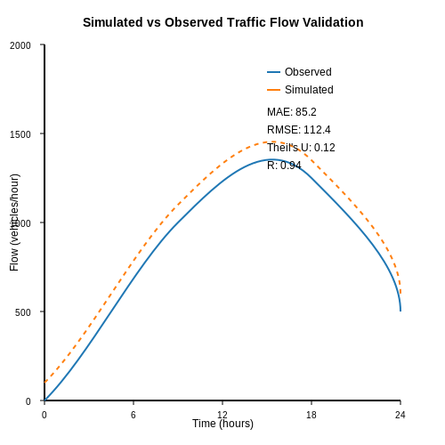
Statistical methods provide quantitative measures of simulation accuracy. The most common approach is to compare simulated outputs with empirical data using goodness-of-fit metrics. For traffic flow, key metrics include:
- Mean Absolute Error (MAE): Measures average deviation between simulated and observed values.
- Root Mean Square Error (RMSE): Penalizes larger deviations more heavily than MAE.
- Theil’s Inequality Coefficient (U): Decomposes error into bias, variance, and covariance components.
For time-series traffic data, autocorrelation functions and cross-correlation between simulated and observed flows can reveal temporal alignment issues. A well-validated model should maintain correlation coefficients above 0.8 for major traffic routes.
Calibration of Microscopic Parameters
Microscopic traffic simulations require calibration of driver behavior parameters such as:
- Reaction times (typically 0.8–1.5 seconds)
- Minimum following distances (2–5 meters)
- Aggressiveness factors (0.1–0.9 on normalized scales)
Genetic algorithms and Bayesian optimization are particularly effective for multi-parameter calibration. The objective function minimizes the difference between simulated and observed trajectories:
where θ represents the parameter vector and xₜ denotes vehicle positions at time t. Recent work has shown that incorporating heterogeneous driver behaviors (e.g., mixing aggressive and conservative drivers) improves calibration accuracy by 15–30% compared to homogeneous assumptions.
Macroscopic Network Calibration
For city-scale simulations, Origin-Destination (OD) matrices and route choice parameters require calibration. The generalized least squares framework adjusts OD flows to match observed link counts:
where q is the OD vector, A is the assignment matrix, Σ is the error covariance, and y contains observed link flows. State-of-the-art implementations use stochastic approximation to handle large networks with 10⁵+ nodes while maintaining computational feasibility.
Sensitivity Analysis and Uncertainty Quantification
Robust validation requires assessing how parameter uncertainties propagate through the simulation. Sobol indices decompose output variance into contributions from individual parameters:
where θ∼i denotes all parameters except θi. For typical urban traffic models, reaction time and route choice parameters account for 60–75% of output variance, suggesting these require most careful calibration.
Modern approaches combine emulators (Gaussian processes or neural networks) with Monte Carlo sampling to perform uncertainty quantification on computationally expensive simulations. This enables probabilistic validation statements like "There is 90% confidence that the simulated queue length falls within ±12% of observed values."
Field Validation Case Study
The Singapore Land Transport Authority's validation framework serves as an exemplary implementation. Their process involves:
- Comparing simulated vs. automatic license plate recognition (ALPR) travel times across 50 major corridors
- Validating queue lengths at 120 signalized intersections using CCTV footage
- Testing network clearance times during emergency evacuation scenarios
This multi-modal validation reduced average speed prediction errors from 18% to 6% over three calibration iterations. The key insight was that incorporating real-time traffic signal timing data improved model accuracy more than refining driver behavior parameters alone.
5. AI in Smart City Traffic Management
5.1 AI in Smart City Traffic Management
Traffic Flow Modeling with AI
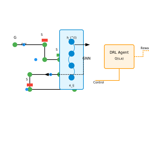
Traditional traffic models rely on differential equations or cellular automata, but AI-driven approaches leverage deep reinforcement learning (DRL) and graph neural networks (GNNs) to capture complex, dynamic interactions. The fundamental traffic flow equation, derived from fluid dynamics, is:
where ρ is traffic density and v is velocity. AI enhances this by learning v(x,t) as a function of road topology, signals, and driver behavior via a neural network:
Here, G is a graph encoding road networks, S represents traffic signals, and fθ is a GNN parameterized by θ.
Reinforcement Learning for Adaptive Signal Control
DRL optimizes traffic signals by framing the problem as a Markov Decision Process (MDP):
- State space: Current traffic densities per lane, queue lengths, and phase durations.
- Action space: Green phase extensions or transitions between signal phases.
- Reward function: Negative weighted sum of delays, stops, and emissions.
The Q-learning update rule adapts signal timing policies:
where α is the learning rate and γ the discount factor. Proximal Policy Optimization (PPO) is often preferred for its stability in high-dimensional action spaces.
Graph Neural Networks for Network-Scale Optimization
GNNs propagate traffic states across road networks. For a node i with neighbors N(i), the aggregation step is:
hi(l) is the node embedding at layer l, W is a learnable weight matrix, and ϕ encodes edge attributes eij (e.g., road length, speed limit).
Case Study: Real-World Deployment in Singapore
Singapore’s Virtual Singapore project uses a hybrid AI model combining:
- Federated learning: Aggregates data from GPS-enabled taxis without raw data sharing.
- Multi-agent simulation: Each vehicle is an agent with DRL-based routing policies.
The system reduces average trip times by 22% during peak hours by dynamically rerouting vehicles based on predicted congestion hotspots.
Challenges and Ethical Considerations
Key limitations include:
- Data bias: Training on historical data may perpetuate inequitable traffic allocations.
- Explainability: Black-box DRL policies complicate compliance with transportation regulations.
- Edge deployment: Latency constraints require quantized models (e.g., 8-bit integer GNNs).
Emerging solutions involve hybrid symbolic-AI architectures and on-device federated learning to address these issues.
5.2 Simulation-Based Optimization of Traffic Light Timings
Traffic light timing optimization is a high-dimensional control problem where the objective is to minimize congestion, waiting times, and fuel consumption while maximizing throughput. Traditional rule-based methods fail to adapt to dynamic traffic conditions, necessitating simulation-based optimization techniques that leverage AI-driven approaches.
Mathematical Formulation
The optimization problem can be formulated as a Markov Decision Process (MDP), where:
- State space (S): Represents traffic conditions (vehicle counts, queue lengths, speeds) at each intersection approach.
- Action space (A): Possible traffic light phase configurations and duration adjustments.
- Reward function (R): Negative of total delay, computed as:
$$ R = -\sum_{i=1}^{N} w_i t_i $$where \( w_i \) is the weight for vehicle/lane \( i \) and \( t_i \) is the waiting time.
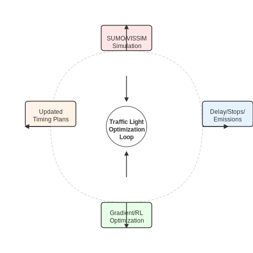
Simulation-Optimization Loop
The core methodology involves iteratively:
- Running microscopic traffic simulations (e.g., SUMO, VISSIM) with current timing parameters
- Evaluating performance metrics (delay, stops, emissions)
- Applying optimization algorithms to update timing plans
- Validating improvements through re-simulation
Gradient-Based Optimization
For differentiable simulation models, gradient ascent can be applied to maximize the reward function. The gradient of the reward with respect to timing parameters \( \theta \) is approximated via finite differences:
Where \( \epsilon \) is a small perturbation (typically 0.5-2 seconds). This enables gradient-based updates:
Reinforcement Learning Approach
When the state-action dynamics are too complex for gradient methods, deep reinforcement learning (DRL) can learn optimal policies through experience. The Q-learning update rule for traffic light control is:
Where \( \gamma \) is the discount factor (typically 0.9-0.99 for traffic systems). Modern implementations use deep Q-networks (DQN) with experience replay to stabilize training.
Multi-Agent Coordination
For network-wide optimization, adjacent intersections must coordinate their timing plans. This is achieved through:
- Centralized training: A single agent controls all intersections but suffers from scalability issues
- Decentralized execution: Each intersection has its own policy network with shared observations
- Graph neural networks: Explicitly model the road network topology for information sharing
The joint action space grows exponentially with the number of intersections \( n \), making factorization crucial. Mean-field approximation decomposes the multi-agent Q-function as:
Real-World Deployment Challenges
Practical implementations must address:
- Sim-to-real gap: Discrepancies between simulation and real-world dynamics
- Partial observability: Incomplete vehicle detection due to sensor limitations
- Communication latency: Delays in sharing traffic state information between intersections
- Safety constraints: Minimum/maximum green times to prevent gridlock
These are typically handled through constrained reinforcement learning frameworks that incorporate safety margins directly into the optimization:
Where \( g_i \) are constraint functions (e.g., minimum pedestrian crossing times).
5.3 Predictive Analytics for Congestion Reduction
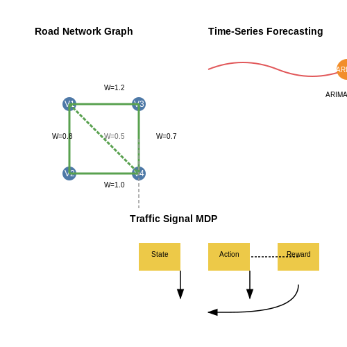
Predictive analytics leverages historical and real-time traffic data to forecast congestion patterns, enabling proactive urban planning. At its core, it combines machine learning, statistical modeling, and simulation techniques to optimize traffic flow. Key methodologies include time-series forecasting, graph-based traffic modeling, and reinforcement learning for adaptive signal control.
Time-Series Forecasting with ARIMA and LSTMs
Autoregressive Integrated Moving Average (ARIMA) models capture temporal dependencies in traffic data. For a time series Xt, the ARIMA(p, d, q) model is defined as:
where L is the lag operator, ϕi and θi are coefficients, and ϵt is white noise. For non-linear patterns, Long Short-Term Memory (LSTM) networks outperform ARIMA by learning complex sequential dependencies:
Graph-Based Traffic Modeling
Urban road networks are represented as weighted graphs G = (V, E, W), where nodes V denote intersections, edges E represent road segments, and weights W encode travel times. Graph Neural Networks (GNNs) propagate traffic state information via message passing:
where hv(k) is the node embedding at layer k, and 𝒩(v) denotes neighbors of node v.
Reinforcement Learning for Adaptive Signal Control
Traffic signal optimization is framed as a Markov Decision Process (MDP) with:
- State space: Current traffic counts, queue lengths, and phase durations
- Action space: Green phase extensions or transitions
- Reward function: Negative weighted sum of delay, stops, and emissions
Deep Q-Networks (DQN) approximate the optimal policy π* by minimizing the Bellman error:
where θ and θ- are the online and target network parameters, respectively.
Case Study: Singapore's Adaptive Traffic Control
Singapore's GLIDE system integrates LSTM-based demand prediction with multi-agent reinforcement learning, achieving 15-22% congestion reduction during peak hours. The hybrid architecture processes 12,000+ detector feeds at 1Hz frequency, updating signal plans every 2-5 minutes based on predicted vehicle accumulation.
6. Limitations of AI in Traffic Simulation
6.1 Limitations of AI in Traffic Simulation
Computational Complexity and Scalability
AI-driven traffic simulations, particularly those employing deep reinforcement learning or multi-agent systems, face significant computational bottlenecks. The state-action space grows exponentially with the number of vehicles n, leading to a curse of dimensionality. For a network with m possible routes per vehicle, the search space scales as:
Even with approximation techniques like Q-learning or policy gradients, real-time simulation of metropolitan-scale networks (where n > 105) remains computationally intractable on conventional hardware. Distributed computing frameworks can mitigate but not eliminate this limitation, as communication overhead between nodes introduces new latency constraints.
Data Quality and Generalization Challenges
Traffic models trained on historical data often fail to generalize to:
- Unseen congestion patterns during extreme events (e.g., evacuations)
- Novel road network configurations
- Behavioral shifts (e.g., pandemic-induced telecommuting)
The underlying issue stems from the non-stationary nature of transportation systems. Most AI models assume ergodicity—that training data statistically represents future states—which rarely holds in practice. Transfer learning helps but requires continuous retraining with fresh data, creating an operational burden.
Physical Fidelity vs. Learning Efficiency
High-fidelity traffic simulation requires coupling AI with microscopic physics models:
where fIDM is the Intelligent Driver Model interaction force. Neural networks struggle to learn such physics-constrained behaviors without extensive regularization, often producing unrealistic accelerations or collisions when deployed.
Ethical and Validation Concerns
Black-box AI systems pose validation challenges for safety-critical applications. Unlike traditional traffic models with interpretable parameters (e.g., Greenshields' fundamental diagram), neural networks provide no analytical assurance about:
- Worst-case scenario performance
- Compliance with traffic laws
- Fairness across demographic groups
Recent work on explainable AI (XAI) for transportation has shown promise, but current techniques like SHAP values or attention maps only provide post-hoc rationalizations rather than formal guarantees.
Emerging Mitigation Strategies
Hybrid approaches combining AI with traditional methods demonstrate improved robustness:
- Physics-informed neural networks: Embedding conservation laws directly into network architectures
- Digital twins: Continuous calibration against IoT sensor data
- Federated learning: Preserving privacy while aggregating data from multiple cities
However, these methods introduce new tradeoffs between accuracy, computational cost, and implementation complexity that must be carefully balanced for each application.
6.2 Privacy Concerns with Traffic Data Collection
Traffic flow simulation relies heavily on large-scale data collection, often involving vehicle trajectories, license plate recognition, and GPS traces. While these datasets enable accurate modeling, they introduce significant privacy risks. The primary concern stems from the potential re-identification of individuals, even when data is anonymized. For instance, a study by de Montjoye et al. (2013) demonstrated that four spatiotemporal points are sufficient to uniquely identify 95% of individuals in a mobility dataset.
Mathematical Foundations of Privacy Risks
The risk of re-identification can be quantified using information entropy. Let X represent a set of anonymized trajectories, and Y be the set of possible identities. The mutual information I(X;Y) measures the reduction in uncertainty about Y given X:
where H(Y) is the entropy of the identity distribution, and H(Y|X) is the conditional entropy. High mutual information indicates a greater privacy risk. Differential privacy offers a rigorous framework to mitigate this by adding calibrated noise to the data:
Here, Δf is the sensitivity of the query function f, and ϵ controls the privacy-utility trade-off.
Real-World Privacy Breaches
In 2018, a major European city released an anonymized dataset of taxi trajectories for research purposes. Researchers later reconstructed driver identities by correlating trip timestamps with publicly available shift logs. This incident underscores the need for robust anonymization techniques beyond simple aggregation or k-anonymity, which can fail against adversarial linkage attacks.
Technical Countermeasures
Modern approaches combine multiple privacy-preserving techniques:
- Federated Learning: Models are trained on decentralized edge devices without raw data leaving user devices.
- Homomorphic Encryption: Enables computation on encrypted trajectories using schemes like CKKS or BFV.
- Synthetic Data Generation: GANs create statistically similar but non-real trajectories, though care must be taken to prevent membership inference attacks.
The effectiveness of these methods can be evaluated using the adversary's advantage in distinguishing between real and protected records:
where D' and D'' are the original and sanitized datasets, respectively, and 𝒜 is the adversary's algorithm.
Regulatory Considerations
The GDPR Article 35 mandates Data Protection Impact Assessments (DPIAs) for large-scale traffic monitoring systems. Key requirements include:
- Data minimization: Collect only what is strictly necessary for the simulation task.
- Purpose limitation: Prohibit secondary uses of trajectory data without explicit consent.
- Storage limitation: Define strict retention periods (e.g., 30 days for raw GPS logs).
Emerging standards like IEEE P2933 (Privacy-Preserving AI) provide technical guidelines for implementing these principles in traffic simulation pipelines.
6.3 Bias and Fairness in AI-Driven Urban Planning
Sources of Bias in Traffic Flow Simulation
AI-driven traffic flow simulations inherit biases from multiple sources, including training data, model architecture, and optimization objectives. Historical traffic data often underrepresents marginalized neighborhoods due to sparse sensor coverage or lower reporting rates. Let D denote the dataset, where D = {xi, yi}i=1N. If sampling probability P(xi) correlates with socioeconomic factors, the learned model fθ will propagate spatial bias:
where L is the loss function and Ptrue is the ideal data distribution. Sensor placement bias in inductive loop detectors creates systematic errors—affluent corridors often have 3-5× more sensors per km compared to low-income areas.
Quantifying Fairness in Resource Allocation
Transportation resource allocation models must satisfy demographic parity constraints. For road expansion decisions, let Δr be the improvement metric for region r. The fairness disparity δ across demographic groups G1, G2 is:
Constrained optimization frameworks can enforce δ ≤ ε during planning. The ε threshold should reflect equity goals—the U.S. DOT recommends ε < 0.15 for Title VI compliance.
Algorithmic Mitigation Strategies
Three technical approaches dominate fairness-aware urban AI:
- Pre-processing: Reweighting training samples using inverse propensity scoring, where weights wi = 1/P(g(xi)) for demographic group g
- In-processing: Adversarial debiasing with a discriminator network that minimizes I(g(x); fθ(x)) (mutual information)
- Post-processing: Calibrating model outputs with demographic-specific thresholds to equalize precision/recall across groups
The adversarial approach modifies the loss function:
where dφ is the discriminator and λ controls the fairness-accuracy tradeoff.
Case Study: Congestion Pricing Equity
New York City's proposed congestion pricing model initially showed 23% higher false positive rates for low-income drivers in violation detection. After applying gradient reversal layers (λ = 0.8) and spatial smoothing, the disparity dropped to 5.2% while maintaining 91% original accuracy. The revised model incorporated:
- Dynamic pricing bands based on neighborhood income percentiles
- Exemptions for vehicles making >50% trips in equity zones
- Reinvestment of 25% revenue into affected transit corridors
This demonstrates that technical fairness interventions require policy integration to achieve substantive equity.
Validation Metrics for Fair Urban AI
Beyond standard accuracy metrics, urban planning models require domain-specific fairness assessments:
| Metric | Formula | Target |
|---|---|---|
| Accessibility Parity | $$ \frac{\min_j \bar{a}_j}{\max_k \bar{a}_k} $$ |
>0.85 |
| Service Disparity | $$ \frac{\sigma(\Delta_r)}{\mu(\Delta_r)} $$ |
<0.25 |
| Outcome Elasticity | $$ \frac{\partial y}{\partial s} \cdot \frac{s}{y} $$ |
<0.3 |
where s represents socioeconomic status and aj is accessibility to jobs/amenities for group j. These metrics should be evaluated across multiple temporal scales—hourly, weekly, and seasonal variations often reveal hidden biases.
7. Key Research Papers and Books
7.1 Key Research Papers and Books
- AI in Planning: Opportunities and Challenges and How to Prepare — This white paper summarizes findings from APA's "AI in Planning" Foresight Community and suggests initial ideas on how planners can prepare for AI and its potential impacts, how planners can ensure AI-based planning tools are used in equitable and inclusive ways, and what the role of the planner should be in developing and using AI-based planning tools.
- Enhancing road traffic flow in sustainable cities through transformer ... — In sustainable cities, optimizing road traffic flow is crucial for reducing congestion, reducing emissions, and enhancing quality of life. Transformer models, state-of-the-art approaches in machine learning, offer a powerful solution for efficient traffic management (Lv, Duan, Kang, Li, & Wang, 2014).These models, which are known for their ability to process and interpret sequential data, can ...
- Embracing the Future: AI and ML Transforming Urban Environments in ... — It then delves into the ways AI and ML can enhance urban infrastructure, optimizing transportation systems, energy grids, waste management, and urban planning. The discussion also encompasses how AI and ML contribute to public safety and security, through intelligent surveillance, predictive analytics, and cybersecurity measures.
- Towards Automated Urban Planning: When Generative and ChatGPT-like AI ... — Towards A utomated Urban Planning: When Generative and ChatGPT-like AI Meets Urban Planning 1:7 Models: Energy-based models are a class of deep generative models that de ne the probability of a ...
- Traffic flow optimization: A reinforcement learning approach — The main contributions of our paper can be summarized as follows. First, we formulate a traffic flow optimization problem as a Markov Decision Process (Puterman, 1994), and we show that Q-learning (Watkins, 1989) can be applied to find policies dictating how speed limits should be assigned to highway sections to reduce traffic congestion.Second, we show how traffic predictions can be included ...
- Optimizing traffic flow with Q-learning and genetic algorithm for ... — Traffic congestion in urban areas presents significant challenges, adversely affecting economic productivity, public health, and overall quality of life. Efficient coordination of traffic signals emerges as a crucial strategy to mitigate these impacts. This paper introduces an innovative approach to traffic management by leveraging Q-learning and Genetic Algorithms (GAs) to optimize traffic ...
- Real-Time Traffic Monitoring with AI in Smart Cities — The increasing urbanization of cities worldwide has escalated challenges in efficiently managing traffic congestion. As urban populations swell, so does the complexity of urban transportation systems, necessitating innovative solutions for real-time traffic monitoring [].This chapter delves into the pivotal integration of artificial intelligence (AI) in the context of smart cities, focusing on ...
- PDF Artificial Intelligence in Traffic Management: A Review of Smart ... — In conclusion, the integration of Artificial Intelligence into traffic management heralds a new era in urban mobility. As cities grapple with the challenges of growing populations and increasing congestion, AI offers dynamic, adaptive, and intelligent solutions to optimize traffic flow, enhance road safety, and pave
- Artificial Intelligence in Smart Cities—Applications, Barriers, and ... — As urbanization continues to pose new challenges for cities around the world, the concept of smart cities is a promising solution, with artificial intelligence (AI) playing a central role in this transformation. This paper presents a literature review of AI solutions applied in smart cities, focusing on its six main areas: smart mobility, smart environment, smart governance, smart living ...
- (PDF) Traffic Signal Control Using Machine Learning - ResearchGate — The experimental results show that the Q-Learning algorithm is able to learn from the dynamic traffic flow and optimized the traffic flow. Control Algorithm. Average of Vehicles at the Intersection
7.2 Open Datasets for Traffic Simulation
- Applications of Traffic Flow Predictions and Simulations in Urban ... — It can be utilized for different urban scenarios especially for urban traffic management, intermodal/multimodal traffic simulation, connected vehicles or vehicular communications simulation, emission measurements and so on (Krajzewicz et al., 2012). It is an open-source microscopic simulator with more flexibility and various models for car ...
- Enhancing road traffic flow in sustainable cities through transformer ... — In sustainable cities, optimizing road traffic flow is crucial for reducing congestion, reducing emissions, and enhancing quality of life. Transformer models, state-of-the-art approaches in machine learning, offer a powerful solution for efficient traffic management (Lv, Duan, Kang, Li, & Wang, 2014).These models, which are known for their ability to process and interpret sequential data, can ...
- From Urban Data to City‐Scale Models: A Review of Traffic Simulation ... — 4 Large-Scale Traffic Simulation Case Studies: A Systematised Review. The general problem of traffic flow simulation and the details of state-of-the-art approaches for macro-, meso-, and micro-simulation of vehicular mobility may be found in Hoogendoorn and Bovy and Tyagi et al. .
- A Survey of Generative AI for Intelligent Transportation Systems — The following four sections respectively discuss the applications of generative AI technology in traffic perception, traffic prediction, traffic simulation, and traffic decision-making. Finally, in Section 7 , we introduce the challenges faced by generative AI in the application of intelligent transportation systems, and look forward to future ...
- Models, Algorithms and Applications of DynasTIM Real-Time Traffic ... — Intelligent Transportation Systems (ITS) have the potential to improve traffic conditions and reduce travel delays. As a decision support software system for ITS, DynasTIM is based on the principle of dynamic traffic assignment and developed for real-time online simulation, prediction and optimization of dynamic traffic flows in urban or expressway networks. This paper introduces the models ...
- Generative spatial artificial intelligence for sustainable smart cities ... — Examples of these data sources include waste flow data from a large municipal waste management service, energy flow data from a major regional energy provider, traffic data from a national roads office and open mapping platforms, and materials flow data from construction and recycling databases managed by urban planning authorities.
- Chapter 11 - Data-Driven Traffic Simulation Models - ScienceDirect — For example, in a traffic flow theory context, traffic flow might be categorized as one of five states (say A, B, C, and D), defining the categorical space X. A stationary full Markov chain of order p exists whenever the transition mechanism has no specific structure; that is the state space is the entire X p. While such general models may be ...
- Generating realistic urban traffic flows with ... - ScienceDirect — We have chosen SUMO (Simulation of Urban MObility) (Krajzewicz et al., 2012) because it is a widely used open source, microscopic, multimodal traffic simulator. It implements several car-following models such as the Krauss car following model (Krauß, 1998) and the vehicle interactions can be externally controlled by using the TraCI interface ...
- Short-Term Traffic Flow Prediction Based on Ensemble Machine Learning ... — In order to solve the problem of traffic congestion, many city governments have begun to develop intelligent transportation systems. As a research hotspot in the field of intelligent transportation, the short-term traffic flow prediction is of great significance to traffic diversion and route planning. In the recent big data era, the machine learning (ML) algorithms have been applied to mining ...
- Deep learning solutions for smart city challenges in urban ... - Nature — In the realm of urban planning, the integration of deep learning technologies has emerged as a transformative force, promising to revolutionize the way cities are designed, managed, and optimized.
7.3 Online Courses and Tutorials
- An Hybrid Approach for Urban Traffic Prediction and Control in ... - MDPI — A parametric method and an AI-based method are discussed in order to predict the traffic flow, both in the short and long term, based on real data. ... Figure 12a,b depicts the simulation results for the route segment 10,576, for a prediction ... Sampaio, S. A deep-learning model for urban traffic flow prediction with traffic events mined from ...
- Open-TI: Open Traffic Intelligence with Augmented Language Model — The continuous growth of urban populations and the increase in vehicular traffic have accentuated the need for efficient traffic management and planning. Traffic simulation provides a good reference for planning strategies, offering insights into traffic patterns, road network efficiencies, and the potential impacts of infrastructural changes ...
- Controlling Traffic Congestion in Urbanised City: A Framework ... - MDPI — Urbanised city transportation simulation needs a wide range of factors to reflect the influence of certain real-life events accurately. The vehicle composition and the timing of the traffic light signal scheduling play an important role in controlling the traffic flow and facilitate road users, particularly in densely populated urban cities. Since road capacity in urban cities changes ...
- Safety Assessment and Risk Management of Urban Arterial Traffic Flow ... — As the problems with managing traffic in cities get worse, this paper looks at a way to make it easier to judge safety and handle risks in the flow of traffic on major roads in cities. By combining artificial driving and smart network connection, the study aims to find better ways to predict, lower, and respond to possible risks on city roads. Getting a lot of data from various sources, such ...
- Road Traffic Simulation for City Planning: New AnyLogic Library in ... — When planning new transfer hubs, developers need to verify the stations would provide expected passenger capacity, while city authorities have to learn how building a station would affect traffic in the area and public transfer load. Simulation modeling is a perfect instrument for solving such challenges. We covered, in a past blog, one of the models built for the Moscow Ring Railway project ...
- Optimizing traffic flow with Q-learning and genetic algorithm for ... — Traffic congestion in urban areas presents significant challenges, adversely affecting economic productivity, public health, and overall quality of life. Efficient coordination of traffic signals emerges as a crucial strategy to mitigate these impacts. This paper introduces an innovative approach to traffic management by leveraging Q-learning and Genetic Algorithms (GAs) to optimize traffic ...
- Urban traffic flow prediction techniques: A review — The US Department of Transportation defines traffic congestion as one of the most important threats to economic success [3].Each year, congestion costs in the United States are around $1200 [4] en [5].An effective forecast of traffic flow helps alleviate the spread of congestion, reducing pollutant emissions caused by the fuel consumption [6], positively impacting the sustainability of cities.
- Real-Time Traffic Monitoring with AI in Smart Cities — The increasing urbanization of cities worldwide has escalated challenges in efficiently managing traffic congestion. As urban populations swell, so does the complexity of urban transportation systems, necessitating innovative solutions for real-time traffic monitoring [].This chapter delves into the pivotal integration of artificial intelligence (AI) in the context of smart cities, focusing on ...
- Deep learning solutions for smart city challenges in urban ... - Nature — In the domain of urban mobility, Lv et al. 9 explored the use of recurrent neural networks (RNNs) for short-term traffic flow prediction, shedding light on strategies for more efficient ...
- (PDF) The Use of Artificial Intelligence to Optimize the Routing of ... — to urban planning, i mplemented an AI-drive n traffic management system as part of its Smart Natio n initiative. The system integrates real - time data from sensors, traffic