Autonomous Drone Flight with AI
1. Core Components of Autonomous Drones
Core Components of Autonomous Drones
Sensor Fusion and Perception
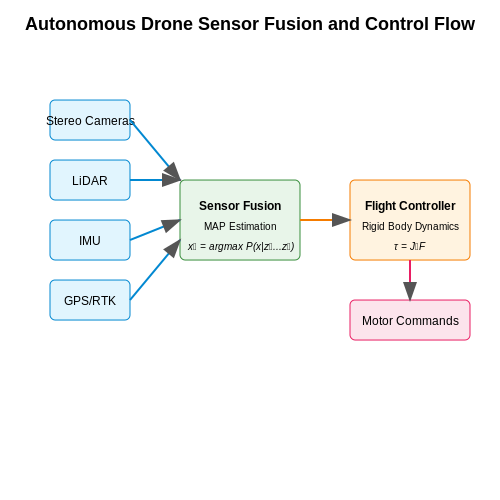
Autonomous drones rely on multi-modal sensor fusion to perceive their environment. The primary sensors include:
- Stereo cameras for depth estimation via disparity mapping, typically achieving 1-5% depth error at 10m range.
- LiDAR (Light Detection and Ranging) with typical angular resolution of 0.1°-0.5° and range accuracy of ±2cm.
- IMUs (Inertial Measurement Units) combining accelerometers and gyroscopes, with MEMS-based units achieving <1° drift/min.
- GPS/RTK for global positioning, where RTK-GPS can achieve centimeter-level accuracy.
The sensor fusion problem can be formulated as a maximum a posteriori (MAP) estimation:
where \(x_t\) is the state vector, \(z_t\) are observations, and \(u_t\) are control inputs. Modern implementations typically use factor graph optimization or deep learning-based fusion networks.
Flight Control Systems
The flight controller solves the rigid body dynamics problem:
where \(p\) is position, \(v\) velocity, \(R\) the rotation matrix, and \(\omega\) angular velocity. Modern controllers use:
- Nonlinear controllers like geometric control or sliding mode control
- Adaptive control for parameter uncertainty
- Learning-based controllers using deep reinforcement learning
Path Planning and Obstacle Avoidance
Optimal path planning solves the minimization problem:
where \(\rho_{obs}\) is an obstacle potential field. State-of-the-art approaches include:
- RRT* (Rapidly-exploring Random Trees) for global planning
- MPC (Model Predictive Control) with 5-20ms time horizons
- Neural planners using CNN or Transformer architectures
Onboard Computing
Modern autonomous drones use heterogeneous computing architectures:
- FPGAs for low-latency sensor processing (1-10ms)
- GPUs for deep learning inference (10-100ms)
- MCUs for real-time control (100μs-1ms)
The computational bottleneck is typically the simultaneous localization and mapping (SLAM) pipeline, which requires solving the visual odometry problem at 30-60Hz:
where \(\pi\) is the camera projection model and \(X_i\) are 3D map points.
Power Systems
Energy optimization considers the power consumption model:
where propulsion power dominates (70-90% of total). The propulsion power follows:
with \(\rho\) air density and \(A\) total rotor area. Modern systems achieve 15-30 minutes flight time with 4-6S LiPo batteries (14.8-22.2V).
Key AI Technologies for Drone Autonomy
Computer Vision for Environmental Perception
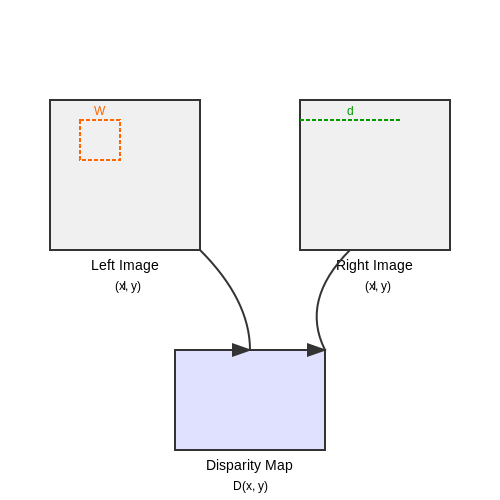
Modern autonomous drones rely heavily on computer vision to interpret their surroundings. Convolutional Neural Networks (CNNs) process visual data from onboard cameras, enabling object detection, semantic segmentation, and depth estimation. The YOLOv5 architecture, for instance, achieves real-time object detection with high precision, critical for obstacle avoidance. For stereo vision, the disparity map D between left and right camera images is computed as:
where W is a local window and d is the disparity range. This enables 3D reconstruction of the environment, essential for path planning.
Reinforcement Learning for Adaptive Control
Deep Reinforcement Learning (DRL) frameworks like Proximal Policy Optimization (PPO) allow drones to learn optimal control policies through trial-and-error interactions. The policy gradient update rule is derived as:
where Ât is the advantage estimate. This approach enables drones to adapt to dynamic wind conditions and payload variations without explicit aerodynamic modeling.
Simultaneous Localization and Mapping (SLAM)
Visual-inertial SLAM systems like ORB-SLAM3 fuse camera and IMU data to maintain localization in GPS-denied environments. The key innovation lies in tightly-coupled nonlinear optimization of the visual-inertial bundle adjustment cost function:
where ρ is the Huber robust cost function, rI and rC are inertial and visual residuals, and Σ represents covariance matrices.
Multi-Sensor Fusion with Kalman Filters
Extended Kalman Filters (EKFs) combine data from LiDAR, radar, and IMUs to maintain accurate state estimation. The prediction and update steps follow:
where Fk is the Jacobian of f, and Hk is the Jacobian of h.
Edge Computing for Real-Time Processing
Jetson Xavier NX modules enable onboard AI inference with TensorRT optimization, achieving 21 TOPS performance while consuming under 15W. The architecture employs mixed-precision quantization:
This reduces model size by 4× while maintaining >95% of FP32 accuracy for critical tasks like emergency landing site detection.
Swarm Intelligence Algorithms
For coordinated drone swarms, bio-inspired algorithms like flocking behavior are implemented through potential fields:
where ka and kr control attraction/repulsion strengths, and da, dr define interaction ranges.
Sensor Fusion and Environmental Perception
Multi-Sensor Data Integration
Autonomous drones rely on heterogeneous sensor arrays—LiDAR, stereo cameras, IMUs, and ultrasonic sensors—each providing partial observations of the environment. Sensor fusion combines these modalities into a unified state estimate through probabilistic frameworks. The core challenge lies in handling asynchronous, noisy measurements with varying precision and update rates.
where Ft is the state transition matrix, Bt the control input matrix, and Ht the observation matrix. Process noise wt ∼ N(0,Qt) and measurement noise vt ∼ N(0,Rt) are modeled as zero-mean Gaussian distributions.
Kalman Filter Variants
For real-time operation, drones employ Kalman filter derivatives:
- Extended Kalman Filter (EKF): Linearizes nonlinear dynamics via first-order Taylor expansion
- Unscented Kalman Filter (UKF): Uses sigma-point transformation for better nonlinear approximation
- Error-State Kalman Filter (ESKF): Separates nominal and error states for improved numerical stability
Deep Learning Approaches
Recent advances integrate neural networks with traditional filters. Attention-based transformer architectures process LiDAR point clouds and camera images through parallel encoders:
Where Q, K, and V represent queries, keys, and values from different sensor modalities. This allows cross-modal feature learning while maintaining geometric constraints.
Obstacle Mapping
Occupancy grid mapping discretizes the environment into probabilistic cells. Each cell's occupancy probability updates via log-odds:
where l0 is the prior log-odds ratio. Modern implementations use 3D voxel grids with octree compression for memory efficiency.
Dynamic Object Tracking
Multi-hypothesis tracking (MHT) associates detected objects across frames while handling occlusions. The probability of association aij between detection i and track j follows:
where Sj is the innovation covariance. Graph neural networks now supplement traditional methods by learning motion patterns from large trajectory datasets.

2. Path Planning and Obstacle Avoidance
Path Planning and Obstacle Avoidance
Optimal Path Planning in Continuous Space
Path planning for autonomous drones involves computing a collision-free trajectory from an initial state qinit to a goal state qgoal in configuration space C. For quadrotors operating in 3D space, C is typically ℝ³ × SO(3), accounting for position and orientation. The problem can be formulated as finding a continuous function:
where Cfree denotes obstacle-free configurations. The Rapidly-exploring Random Tree (RRT*) algorithm provides probabilistic completeness guarantees for this problem. At each iteration, RRT*:
- Samples a random configuration qrand
- Finds the nearest node qnear in the current tree
- Extends toward qrand by a step size Δq
- Rewires nearby nodes if a lower-cost path is found
Dynamic Obstacle Avoidance with Velocity Obstacles
For moving obstacles, the velocity obstacle (VO) formulation provides real-time avoidance. Given a drone at position p with velocity v and an obstacle at pobs with velocity vobs, the collision cone CC is defined as:
where r terms represent radii. The set of avoiding velocities is the complement of CC. For multiple obstacles, the feasible velocity space becomes:
where Vmax represents the drone's dynamic constraints. The optimal avoiding velocity is selected by minimizing a cost function incorporating goal direction and smoothness.
Deep Reinforcement Learning for Adaptive Navigation
Recent advances employ deep reinforcement learning (DRL) to learn navigation policies directly from sensor inputs. The policy πθ maps raw observations ot to actions at, trained to maximize expected return:
Key design choices include:
- Observation space: Typically includes depth images, lidar scans, or compressed latent representations
- Action space: Either low-level motor commands or high-level velocity waypoints
- Reward shaping: Combines goal progress, collision penalties, and motion smoothness terms
Proximal Policy Optimization (PPO) has demonstrated particular success in this domain due to its stability with continuous action spaces. The policy update is constrained by:
where rt is the probability ratio between new and old policies, and Ât is the advantage estimate.
Multi-Sensor Fusion for Robust Perception
Reliable obstacle detection requires fusing data from multiple sensors. A typical setup combines:
- Stereo vision: Provides dense depth estimates up to 20m with ~5% error
- Time-of-flight lidar: Offers precise ranging (1-2cm accuracy) but sparse sampling
- Ultrasonic sensors: Effective for close-range (0.1-5m) transparent obstacle detection
The sensor fusion pipeline often employs an Extended Kalman Filter (EKF) with measurement models:
where h represents the nonlinear observation models and R the measurement noise covariance matrices. The EKF recursively updates the state estimate x̂t and covariance Pt:
where H is the Jacobian of h evaluated at the prior estimate.

2.2 Reinforcement Learning for Flight Control
Markov Decision Process Formulation
Reinforcement learning (RL) frames drone flight control as a Markov Decision Process (MDP), defined by the tuple (S, A, P, R, γ), where:
- S represents the state space (position, velocity, orientation)
- A is the action space (motor thrusts, control surface deflections)
- P(s'|s,a) defines state transition probabilities
- R(s,a) is the immediate reward function
- γ ∈ [0,1] is the discount factor
The optimal policy π* maximizes the expected cumulative reward, with Q*(s,a) representing the optimal action-value function.
Policy Gradient Methods
For continuous control tasks like drone flight, policy gradient methods directly optimize a parameterized policy πθ(a|s). The gradient of the expected return J(θ) is:
where τ is a trajectory and Ât is the advantage estimate. Proximal Policy Optimization (PPO) has shown particular success in drone control due to its stability:
Reward Function Design
Effective reward functions for drone flight balance multiple objectives:
- Position tracking: Rpos = -||ptarget - pdrone||2
- Orientation stability: Ratt = -||qdesired - qactual||
- Energy efficiency: Renergy = -Σ|ui|2
- Collision avoidance: Binary penalty for proximity violations
Simulation-to-Reality Transfer
Domain randomization addresses the sim-to-real gap by varying parameters during training:
- Mass and inertia properties (±10%)
- Motor dynamics (time constants, thrust coefficients)
- Environmental conditions (wind, turbulence)
- Sensor noise characteristics
The dynamics randomization loss function:
where ξ represents randomized parameters sampled from distribution Ξ.
Hierarchical Reinforcement Learning
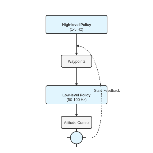
For complex navigation tasks, a two-level hierarchy proves effective:
- High-level policy: Generates waypoints at 1-5 Hz
- Low-level policy: Executes attitude control at 50-100 Hz
The temporal abstraction is formalized through options framework:
where I ⊆ S is the initiation set, π is the option policy, and β is the termination condition.
Real-World Implementation Challenges
Practical deployment requires addressing:
- Partial observability: Solved through recurrent policies or belief state estimation
- Computation constraints: Quantized neural networks for embedded deployment
- Safety guarantees: Barrier functions to constrain actions
where h is a control barrier function and γ determines the safety margin.
2.3 Computer Vision for Real-Time Decision Making
Real-time computer vision enables autonomous drones to perceive and interpret their environment dynamically. Key algorithms include object detection, semantic segmentation, and optical flow estimation, each requiring optimized implementations to meet latency constraints. The computational pipeline typically involves frame capture, preprocessing, feature extraction, and decision inference, with end-to-end latencies often constrained to under 50ms for agile flight.
Feature Extraction and Optical Flow
Optical flow estimation calculates per-pixel motion vectors between consecutive frames, critical for obstacle avoidance and stabilization. The Lucas-Kanade method solves the optical flow equation by assuming local constancy in a window:
where Ix, Iy are spatial derivatives, It is the temporal derivative, and u, v represent flow vectors. For real-time performance, pyramidal implementations reduce computational complexity from O(n2) to O(n log n).
Deep Learning Architectures for Latency-Constrained Environments
EfficientNet variants balance accuracy and inference speed through compound scaling of depth, width, and resolution. The baseline MobileNetV3 achieves 3.8× faster inference than ResNet-50 on embedded GPUs, with architectural optimizations including:
- Squeeze-and-excitation blocks for channel-wise attention
- Hard-swish activations replacing ReLU
- Neural architecture search (NAS)-optimized layer configurations
Quantization-aware training further reduces model footprints, with INT8 quantization typically yielding 4× memory reduction and 2-3× speedup on TensorRT-optimized platforms.
Sensor Fusion with Inertial Measurement Units
Visual-inertial odometry (VIO) combines monocular/stereo vision with IMU data through tight coupling in Kalman filters or factor graphs. The error state Kalman filter (ESKF) formulation propagates state estimates as:
where δx is the error state, Fk the state transition matrix, and wk process noise. Tightly-coupled approaches demonstrate 40% lower drift than loosely-coupled methods at 200Hz update rates.
Hardware Acceleration Strategies
Jetson AGX Orin's 2048 CUDA cores and 64 Tensor Cores enable 275 TOPS performance for vision pipelines. Key optimization techniques include:
- Half-precision (FP16) inference with layer-wise scaling
- Tensor core-optimized GEMM operations
- Async DMA transfers overlapping compute and memory operations
On FPGA platforms, Vivado HLS can pipeline vision algorithms achieving 8× throughput improvement over CPU implementations through loop unrolling and dataflow optimization.

3. Hardware and Software Integration
3.1 Hardware and Software Integration
Sensor Fusion and Embedded Processing
Autonomous drones rely on multi-modal sensor fusion to achieve robust state estimation. A typical setup integrates:
- IMU (Inertial Measurement Unit): Accelerometers and gyroscopes provide high-frequency (200Hz–1kHz) but noisy motion data. The raw measurements follow:
where RWB is the rotation from body to world frame, b denotes biases, and η represents Gaussian noise.
- Visual Odometry: Monocular or stereo cameras (30–60Hz) enable feature-based SLAM. The reprojection error minimized in bundle adjustment is:
with π as the camera projection model and TWC the camera pose.
Real-Time AI Inference Pipeline
Onboard neural networks for obstacle avoidance or object tracking require hardware-software co-design:
| Component | Latency Budget | Power Constraint |
|---|---|---|
| Jetson Xavier NX | <10ms (per frame) | 15W TDP |
| Qualcomm RB5 | <20ms | 7W TDP |
Quantization-aware training is critical for edge deployment. A typical INT8 quantization scheme maps float32 activations:
Middleware Architecture
ROS 2 with DDS ensures deterministic communication between modules:
  // QoS profile for critical control messages
  auto qos = rclcpp::QoS(rclcpp::KeepLast(10))
    .reliable()
    .deadline(std::chrono::milliseconds(5))
    .durability_volatile();
Time synchronization across sensors uses PTP (IEEE 1588) with hardware timestamping to achieve <100μs skew.
Fail-Safe Mechanisms
Redundant flight controllers implement voting systems. The Markov decision process for failover:
where s represents system states (normal, degraded, critical) and a includes actions like throttle reduction or emergency landing.

3.2 Simulation and Testing Environments
Physics-Based Simulation Frameworks
High-fidelity physics engines such as Gazebo, AirSim, and PyBullet are critical for simulating drone dynamics before real-world deployment. These frameworks solve the rigid-body dynamics equations of motion, incorporating aerodynamics, sensor noise, and environmental disturbances. The Newton-Euler equations governing drone motion are:
where F is the net force, τ is the torque vector, I is the inertia tensor, and ω is angular velocity. Gazebo implements these equations with ODE or Bullet solvers, while AirSim uses Unreal Engine's physics with custom rotor models.
Sensor Simulation and Noise Modeling
Realistic sensor simulation requires modeling:
- IMU biases (Gaussian random walk)
- GPS multipath errors (Rayleigh-distributed)
- Camera lens distortion (Brown-Conrady model)
The accelerometer noise model in AirSim follows:
where ba is the bias (modeled as ba(t) = ba(t-1) + σrwΔw) and na is white noise with PSD Sa(f) = Na.
Hardware-in-the-Loop (HITL) Testing
HITL systems bridge simulation and reality by connecting actual flight controllers (e.g., Pixhawk) to simulated environments. The signal flow involves:
Critical considerations include:
- Jitter compensation for PWM signal timing
- Deterministic execution of simulation steps
- Latency matching between simulated and real sensors
Photorealistic Rendering for Vision Systems
Training vision-based navigation algorithms requires synthetic data with:
- Procedural city generation (e.g., using CARLA's OpenDRIVE maps)
- Dynamic lighting conditions (ray-traced shadows)
- Domain randomization for texture variations
The rendering pipeline in NVIDIA Omniverse follows:
def render_scene(drone_pose):
   # RTX-accelerated path tracing
   with omni.kit.rtx.RenderContext() as ctx:
      ctx.set_camera(drone_pose)
      return ctx.render(
         samples=64,
         denoiser="OptiX",
         physics_dt=1/120.0
      )
Validation Metrics
Simulation-to-reality (Sim2Real) transfer quality is quantified using:
where R are rotation matrices. Industry benchmarks typically require εpos < 0.5m and εatt < 5° for waypoint navigation tasks.
Edge Computing for Onboard AI Processing
Computational Constraints in Autonomous Drones
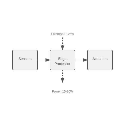
Autonomous drones require real-time processing of high-dimensional sensor data (e.g., LiDAR, cameras, IMU) while adhering to strict power and weight constraints. Traditional cloud-based AI inference introduces latency and dependency on network connectivity, making edge computing essential. The computational efficiency of onboard processing is governed by the following trade-offs:
For a typical convolutional neural network (CNN) processing 640×480 RGB images at 30 FPS, the required throughput exceeds 200 GOPS (Giga Operations Per Second). Edge devices like the NVIDIA Jetson AGX Orin (275 TOPS) or Qualcomm QCS8550 (48 TOPS) meet these demands while operating under 30W power budgets.
Hardware Architectures for Edge AI
Modern edge AI processors employ heterogeneous architectures combining:
- Vector processors (e.g., ARM NEON, Intel AVX) for parallelizable tensor operations
- Fixed-function accelerators (e.g., NPUs, TPUs) for matrix multiplications
- Low-power CPU clusters for control logic
The energy efficiency (GOPS/W) of these architectures follows:
where IPC is instructions per cycle and Ceff is the effective switched capacitance. For example, the Google Edge TPU achieves 4 TOPS at 2W (η = 2000 GOPS/W) through 8-bit integer quantization and systolic array design.
Model Optimization Techniques
Neural network models must be optimized for edge deployment:
Quantization
Reducing precision from FP32 to INT8 cuts memory bandwidth by 4× while maintaining <90% accuracy for most CNNs. The quantization error εQ is bounded by:
where Δ is the quantization step size and L is the loss function.
Pruning
Iterative magnitude pruning removes weights below threshold θ:
with T being total pruning steps. This achieves >80% sparsity in ResNet-50 with <1% accuracy drop.
Real-World Deployment Challenges
Field testing reveals three critical edge cases:
- Thermal throttling: Processor clocks reduce by 15-25% at >85°C ambient temperatures
- Memory bottlenecks: DDR4 bandwidth (25.6 GB/s) becomes limiting for multi-model pipelines
- Power transients: LiPo battery sag during high-thrust maneuvers causes voltage drops below IC specifications
Mitigation strategies include model partitioning across CPU/GPU/NPU and adaptive clock gating based on thermal sensors.
4. Safety and Regulatory Compliance
4.1 Safety and Regulatory Compliance
Risk Assessment and Mitigation
Autonomous drones must operate within a probabilistic safety framework to minimize risks to humans, infrastructure, and other aircraft. The fundamental risk metric is the probability of catastrophic failure per flight hour (Pfail), which regulatory bodies typically cap at 10-7 for urban operations. This requires:
- Redundant sensor suites (LiDAR, radar, stereo vision) with independent failure modes
- Formal verification of control algorithms using temporal logic (e.g., Linear Temporal Logic)
- Real-time monitoring of system health through Bayesian fault detection
where λi represents the failure rate of subsystem i and t is exposure time. For n=5 redundant systems each with λ=10-5/hour, Pfail ≈ 5×10⁻⁵ over 1 hour - still above aviation safety thresholds, necessitating additional safeguards.
Regulatory Frameworks
Current regulations evolve through three key paradigms:
- Geofencing: Digital perimeter enforcement via GNSS/RTK with cryptographic signature verification
- Dynamic Airspace Allocation: UTM (UAS Traffic Management) systems implementing contract-based separation
- Certification Requirements: DO-178C for software, DO-254 for hardware in aviation contexts
The FAA's Remote ID rule (14 CFR Part 89) mandates broadcast of:
- EUROCAE ED-269 compliant identity packets
- WSG84 coordinates with < 1m horizontal accuracy
- Velocity vector updated at ≥1Hz
Collision Avoidance Systems
Modern implementations use hybrid approaches combining:
- Rule-based: Velocity obstacles (VO) for deterministic scenarios
- Learning-based: Deep reinforcement learning (DRL) with safety layers
The collision cone formulation for a dynamic obstacle:
where θc is the minimum avoidance angle and vrel the relative velocity. DRL policies are typically trained with constrained optimization:
Emergency Procedures
Autonomous drones must implement fail-safe behaviors verifiable through model checking tools like NuSMV. A typical state machine includes:
Key transitions include battery threshold triggers (≤20% capacity) activating return-to-home (RTH) protocols with adaptive path planning that accounts for wind fields:
where w represents wind disturbances and B the disturbance input matrix. The RTH trajectory is recalculated using convex optimization with time-varying safety margins.

4.2 Privacy Concerns in Autonomous Drone Operations
Data Collection and Surveillance Risks
Autonomous drones equipped with high-resolution cameras, LiDAR, and other sensors can inadvertently capture sensitive data, raising significant privacy concerns. The primary issue stems from the indiscriminate nature of aerial data collection, where drones may record private property, individuals, or activities without explicit consent. Advanced computer vision algorithms exacerbate this by enabling facial recognition, object tracking, and behavioral analysis, which can be repurposed for unauthorized surveillance.
The risk is quantified by the privacy intrusion potential (PIP), a metric derived from the sensor's resolution, field of view, and AI processing capabilities:
where R is the sensor resolution (pixels), FOV is the field of view (radians), α is the AI processing factor (0 to 1), and D is the distance to the target (meters). Higher PIP values indicate greater privacy risks.
Legal and Regulatory Challenges
Existing privacy laws, such as the General Data Protection Regulation (GDPR) in the EU and the Fourth Amendment in the US, were not designed with autonomous drones in mind. Key legal ambiguities include:
- Airspace vs. Property Rights: Drones operating in public airspace may still capture private property data, leading to conflicts over ownership and consent.
- Data Retention Policies: Lack of standardized rules for how long drone-captured data can be stored, especially when AI systems process it in real-time.
- Anonymization Feasibility: Even with techniques like blurring or encryption, AI can often reconstruct identities from partial data.
Technical Mitigation Strategies
Several AI-driven approaches can reduce privacy risks without compromising operational efficiency:
1. Differential Privacy in Drone Data
By adding controlled noise to collected data, differential privacy ensures that individual identities cannot be inferred while preserving aggregate insights. For a dataset X, the privacy guarantee is:
where ℳ is the mechanism, ϵ is the privacy budget, and X' is a neighboring dataset.
2. Onboard Edge Processing
Running AI models locally on the drone's hardware (e.g., NVIDIA Jetson or Qualcomm Flight RB5) minimizes data transmission risks. Federated learning can further enhance privacy by aggregating model updates instead of raw data.
3. Geofencing and Ethical AI Constraints
Hard-coded no-fly zones and real-time ethical filters can prevent drones from capturing restricted areas. For example, a convolutional neural network (CNN) can classify and redact sensitive objects (e.g., faces, license plates) before storage.
Case Study: Privacy Violations in Urban Drone Delivery
A 2023 study of drone delivery services in Tokyo revealed that 17% of flights inadvertently captured private indoor spaces through windows. The incident prompted revisions to Japan's UAV Privacy Act, mandating stricter altitude limits and oblique camera angles in residential areas.
Emerging Research in Privacy-Preserving AI
Recent advances include:
- Homomorphic Encryption: Allows AI to process encrypted drone data without decryption, though computational overhead remains high.
- Zero-Knowledge Proofs: Enables drones to verify compliance with privacy policies without revealing raw data.
- Adversarial Privacy: AI models trained to generate "privacy-preserving" sensor noise that disrupts unauthorized analysis.
4.3 Mitigating Bias in AI-Driven Flight Systems
Sources of Bias in Autonomous Drone Navigation
Bias in AI-driven flight systems arises from multiple sources, including skewed training datasets, algorithmic design choices, and sensor limitations. Training data may underrepresent edge cases, such as rare weather conditions or unusual obstacles, leading to poor generalization. Algorithmic bias can emerge from improper loss function weighting, where certain scenarios (e.g., urban vs. rural environments) are prioritized disproportionately. Sensor biases, such as LiDAR’s reduced accuracy in fog, compound these issues.
Here, wi represents biased weights favoring overrepresented data points, and ℓ is the loss function. Mitigation requires reweighting or resampling to balance contributions across scenarios.
Algorithmic Fairness in Path Planning
Path-planning algorithms must account for spatial fairness to avoid systemic exclusion of certain regions. A common issue is over-optimization for energy efficiency, which may neglect underserved areas. The fairness-aware objective function incorporates a fairness penalty λF:
where KL is the Kullback-Leibler divergence between the coverage distribution Pcoverage and a uniform distribution U. This ensures equitable service across all regions.
Sensor Fusion for Bias Reduction
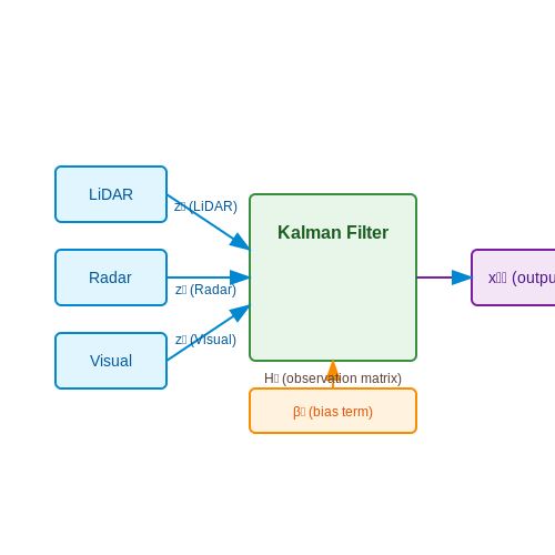
Multimodal sensor fusion mitigates individual sensor biases. For instance, combining visual, LiDAR, and radar data reduces dependency on any single modality. A Kalman filter variant with bias-aware updates is often employed:
Here, βk explicitly models sensor bias, estimated online via expectation-maximization. This adjusts predictions dynamically, improving robustness.
Case Study: Bias in Urban vs. Rural Terrain
A 2023 study by ETH Zurich revealed that drones trained primarily in urban environments exhibited 23% higher collision rates in rural areas due to sparse tree representations in training data. The solution involved adversarial training with a terrain classifier to force uniform feature extraction:
where G generates rural-like features from urban data, and D discriminates between real and generated features. This reduced the performance gap to 5%.
Real-Time Bias Monitoring
Embedded bias detectors use statistical divergence metrics to flag deviations from expected behavior. For example, a χ²-test compares observed obstacle detection rates with historical averages:
Threshold breaches trigger model recalibration or human-in-the-loop intervention. NVIDIA’s DRIVE OS implements this for safety-critical aviation systems.
5. Key Research Papers and Articles
5.1 Key Research Papers and Articles
- PDF DrIFT: Autonomous Drone Dataset with Integrated Real and Synthetic Data ... — Table 1. Drone Datasets: The DrIFT dataset, as the first drone de-tection dataset to study four DSs, includes image frames with mul-tiple drones, real and synthetic data, and ground and aerial PoVs. The "#DS" indicates the number of types of DSs studied. 2. Related Work 2.1. Drone Datasets Drone datasets have recently become publicly avail-
- Unmanned aerial vehicles (UAVs): practical aspects, applications, open ... — This article focuses on open-source flight controllers for research purpose. It addresses both software and hardware controllers and several other components for UAVs ... 0.5-1: 50-9000 > 250: 250-2500: Open in a new tab. Table 8. Feature-based comparison of UAVs. UAV type Altitude (km) ... https://dronehub.ai; 61. HIVE. Autonomous Drone ...
- Fully neuromorphic vision and control for autonomous drone flight - Science — Figure 6B shows landing with divergence ν z, sp B = − 0.5 1/s for various lighting conditions (quantified with lux measurements). With these experiments, we aimed to investigate the robustness of the approach to wildly varying event statistics. ... A particularly promising avenue to autonomous flight of such tiny drones is to make the entire ...
- Artificial Intelligence Applied to Drone Control: A State of the Art - MDPI — The integration of Artificial Intelligence (AI) tools and techniques has provided a significant advance in drone technology. Besides the military applications, drones are being increasingly used for logistics and cargo transportation, agriculture, construction, security and surveillance, exploration, and mobile wireless communication. The synergy between drones and AI has led to notable ...
- DESIGN AND DEVELOPMENT OF AI-BASED AUTONOMOUS DRONE - ResearchGate — autonomous flight controller for automatic aerial maneuvering and cutting-edge AI object detection for task execution. By integrating these components seamlessly, the system will
- (PDF) Flying Free: A Research Overview of Deep Learning in Drone ... — A typical quad rotor helicopter drone, constructed for autonomous flight research. Level of autonomous drone navigation mapped by functional features. A categorisation of Level 4 autonomous ...
- Artificial Intelligence-Based Autonomous UAV Networks: A Survey - MDPI — The survey focused on key aspects of UAV autonomous features, network resource management, channel access, routing protocols, security, and privacy management. Research findings show that AI-based autonomous UAV networks are a technologically viable paradigm for providing a cost-effective solution in the design and deployment of next-generation ...
- Cost-Effective Autonomous Drone Navigation Using Reinforcement ... - MDPI — Artificial intelligence (AI) is used in tasks that usually require human intelligence. The motivation behind this study is the growing interest in deploying AI in public spaces, particularly in autonomous vehicles such as flying drones, to address challenges in navigation and control. The primary challenge lies in developing a robust, cost-effective system capable of autonomous navigation in ...
- UAV swarms: research, challenges, and future directions — Unmanned Aerial Vehicle (UAV) swarms represent a transformative advancement in aerial robotics, leveraging collaborative autonomy to enhance operational capabilities. This paper provides a comprehensive exploration of UAV swarm infrastructure, recent research advancements, and diverse applications. Key areas such as coordinated path planning, task assignment, formation control, and security ...
- (PDF) Unmanned Aerial Vehicles (UAVs): Practical aspects, applications ... — Recently, unmanned aerial vehicles (UAVs) or drones have emerged as a ubiquitous and integral part of our society. They appear in great diversity in a multiplicity of applications for economic ...
5.2 Open-Source Projects and Tools
- Top 23 Drone Open-Source Projects - LibHunt — Which are the best open-source Drone projects? This list will help you: ardupilot, PX4-Autopilot, gobot, openMVG, ODM, ExpressLRS, and qgroundcontrol. ... GAAS is an open-source program designed for fully autonomous VTOL(a.k.a flying cars) and drones. ... dRehmFlight. 11 14 1,171 2.9 C++ Teensy/Arduino flight controller and stabilization for ...
- GitHub - alexkoven/Autonomous-UAVs: List of open-source algorithms and ... — autoware.ai: self-driving vehicles: dronet: learning to fly: ETH: deep learning trained from cars to predict steering angle, collision prob: ️: Deep RL w Airsim: allows RL with Airsim: Autonomous UAV swarms: autonomous-drone: enable autonomous drone delivery w Aero RTF and PX4: ️: PEDRA: Georgia Tech: RL for drones with unreal engine: drif ...
- Home - AirSim - GitHub Pages — Welcome to AirSimExt (aka AirSimExtensions)# AirSimExt is a simulator for drones, cars and more, built on Unreal Engine 5.2. It is open source, cross platform, and supports software-in-the-loop simulation with popular flight controllers such as PX4 and ArduPilot and hardware-in-loop with PX4 for physically and visually realistic simulations.
- nikulram/Advanced-Autonomous-Drone-Navigation-System — An advanced autonomous drone navigation system using complex technologies in computer vision and AI for real-time obstacle detection, environmental interaction, and adaptive flight path management. ... Algorithms dynamically adjust the drone's flight path based on real-time ... The contributors and maintainers of all used open-source software ...
- GitHub - microsoft/AirSim: Open source simulator for autonomous ... — AirSim is a simulator for drones, cars and more, built on Unreal Engine (we now also have an experimental Unity release). It is open-source, cross platform, and supports software-in-the-loop simulation with popular flight controllers such as PX4 & ArduPilot and hardware-in-loop with PX4 for physically and visually realistic simulations.
- Top 23 Quadcopter Open-Source Projects - LibHunt — Which are the best open-source Quadcopter projects? This list will help you: ExpressLRS, inav, cleanflight, Low-Cost-Mocap, gym-pybullet-drones, rotors_simulator, and esp-drone. ... hardware and documentation for my autonomous quad copter project Project mention: Peng ... I'm making a raspberry pi drone, what flight controller can I get for ...
- Open Source Autopilot for Drones - PX4 Autopilot — PX4 is an open source flight control software for drones and other unmanned vehicles. The project provides a flexible set of tools for drone developers to share technologies to create tailored solutions for drone applications. PX4 is hosted by Dronecode, a Linux Foundation non-profit.
- Copter documentation - ArduPilot — Success with Copter requires that the 'First Time Setup' and 'First Flight and Tuning' sections of this documentation be read and followed! This is the full-featured, open-source multicopter UAV controller that won the Sparkfun 2013 and 2014 Autonomous Vehicle Competition (dominating with the top five spots).
- ArduPilot - Versatile, Trusted, Open — ArduPilot is a trusted, versatile, and open source autopilot system supporting many vehicle types: multi-copters, traditional helicopters, fixed wing aircraft, boats, submarines, rovers and more. The source code is developed by a large community of professionals and enthusiasts. New developers are always welcome! The best way to start is by joining the Developer Team Forum, which is open to ...
- GitHub - ArduPilot/ardupilot: ArduPlane, ArduCopter, ArduRover, ArduSub ... — The ArduPilot project is open source and we encourage participation and code contributions: guidelines for contributors to the ardupilot codebase. We have an active group of Beta Testers to help us improve our code: release procedures. Desired Enhancements and Bugs can be posted to the issues list.
5.3 Recommended Books and Courses
- 6 books on AI for Drones [PDF] — These books are dedicated to drone AI software development, navigation systems and sensor integration. By studying these books, startup specialists can better understand how AI can optimize flight paths, enable advanced data analysis, and improve the efficiency and safety of various applications, from agriculture and infrastructure inspection to search and rescue...
- Intelligent Autonomous Drones with Cognitive Deep Learning: Build AI ... — What is an artificial intelligence (AI)-enabled drone and what can it do? Are AI-enabled drones better than human-controlled drones? This book will answer these questions and more, and empower you to develop your own AI-enabled drone.
- Robotics, Autonomous Vehicles, Drones, and Artificial Intelligence — This course explores the field of robotics, autonomous vehicles, and drones, and exposes students to the core technologies and systems through practical exercises and simulation. These are fields with tremendous growth and opportunities in the next 10-50 years; billions of dollars are being invested and the market size is expected to grow 10-15 percent annually. The impact of these ...
- PDF Unmanned Air Systems: UAV Design, Development and Deployment — The UAV will probably have a more sophisticated electronic flight control system compared with the manned aircraft and, of course, a day/night surveillance camera system rather than an observer with a pair of binoculars, night vision goggles and digital SLR camera.
- Drone Technology | Wiley Online Books — DRONE TECHNOLOGY This book provides a holistic and valuable insight into the revolutionary world of unmanned aerial vehicles (UAV). The book elucidates the revolutionary and riveting research in the ultramodern domain of drone technologies, drone-enabled IoT applications, and artificial intelligence-based smart surveillance. The book explains the most recent developments in the field ...
- 8 Best Books on Drones for You to Get Started in 2025 — A drone is a modern aerial vehicle that is capable of recording visual and audio data, mapping locations, using firearms on targets, and much more. Drones are become very popular in recent years. Earlier drone technology was only known to the military but now a common man like you can build a drone at home.
- Mastering Drone Technology with AI: A comprehensive guide to drone ... — The book gives readers a thorough knowledge of cutting-edge advancements including Machine Learning, computer vision, and autonomous flight systems, making it an indispensable resource for anybody interested in the convergence of AI and unmanned aerial vehicles (UAVs).
- The Best Drones Books of All Time - BookAuthority — The best drones books recommended by Romeo Durscher, such as Drone Warrior, FPV Flight Dynamics, Eyes over the World and Remote Pilot Test Prep.
- Intelligent Autonomous Drones with Cognitive Deep Learning — This book examines the detailed process to develop fully autonomous drones that incorporates object-oriented design and cognitive deep learning systems.
- Drone Technology - Scrivener Publishing — The book also has a fascinating chapter on application intrusion detection by drones using recurrent neural networks. Other chapters address interdisciplinary fields like artificial intelligence, deep learning, the role of drones in healthcare in smart cities, and the importance of drone technology in agriculture.