Federated Learning: Privacy-Preserving ML
1. Definition and Core Principles
Definition and Core Principles
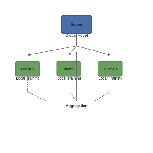
Federated Learning (FL) is a decentralized machine learning paradigm where model training occurs across multiple devices or servers holding local data samples, without exchanging the raw data itself. Instead of centralizing data in a single location, FL enables collaborative training by aggregating model updates from participating nodes, preserving data privacy by design. This approach is particularly valuable in scenarios where data cannot be shared due to regulatory constraints (e.g., GDPR, HIPAA) or ethical considerations.
Mathematical Formulation
The core optimization problem in federated learning can be expressed as minimizing a global objective function F(w), where w represents the model parameters. The global objective is typically a weighted average of local objectives from K participating clients:
where nk is the number of samples on client k, N is the total number of samples across all clients, and Fk(w) is the local objective for client k. Each client computes updates to w based on its local data, and only these updates (not the raw data) are shared with a central server for aggregation.
Key Principles
Federated learning operates on three foundational principles:
- Data Decentralization: Training data remains distributed across edge devices or siloed servers, never leaving its original location.
- Local Computation: Each participant computes model updates using its local data, typically via stochastic gradient descent (SGD) or variants.
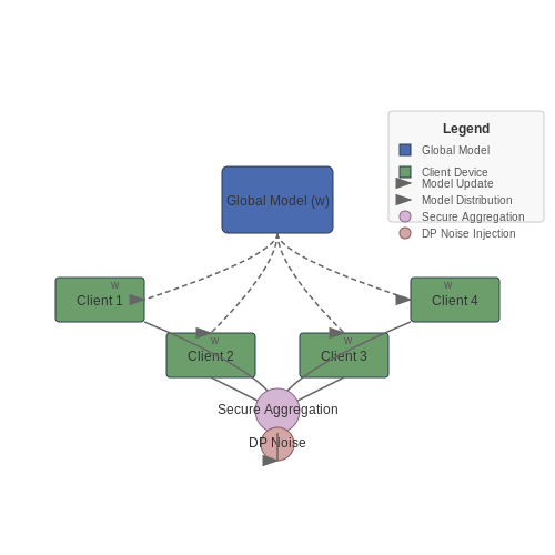
- Secure Aggregation: Model updates are combined through cryptographic protocols (e.g., secure multi-party computation) or differential privacy mechanisms to prevent reconstruction of raw data from gradients.
Communication-Efficient Training
The federated averaging (FedAvg) algorithm reduces communication overhead by performing multiple local SGD steps before aggregation. For client k with learning rate η, the local update after τ steps is:
The server then computes a weighted average of these updates:
This process iterates until convergence, with careful tuning required to balance communication rounds and local computation.
Privacy Guarantees
FL provides formal privacy assurances through:
- Differential Privacy (DP): Adding calibrated noise to gradients or model updates to prevent data leakage, satisfying (ε, δ)-DP guarantees.
- Secure Aggregation: Cryptographic protocols that prevent the server from inspecting individual updates while correctly computing the aggregate.
- Homomorphic Encryption: Enabling computation on encrypted model parameters, though with significant computational overhead.
The privacy-accuracy trade-off is governed by parameters like DP noise magnitude and aggregation frequency, requiring careful optimization for each application domain.
System Heterogeneity
Practical FL systems must account for variability in:
- Hardware Capabilities: Differences in compute resources across devices (e.g., smartphones vs. servers).
- Network Conditions: Unreliable or slow connections that may delay or drop participant updates.
- Data Distribution: Non-IID data partitions where local datasets are not representative of the global distribution.
Advanced techniques like adaptive client selection and staleness-aware aggregation help maintain model performance under these constraints.

1.2 Key Components: Clients, Server, and Aggregation
Client-Side Model Training
In federated learning, clients (e.g., edge devices, mobile phones, or IoT sensors) perform local model training on their private datasets. Each client k computes a model update Δθk by minimizing a local loss function Lk(θ) via stochastic gradient descent (SGD). The update rule for client k at iteration t is:
where η is the learning rate. Unlike centralized training, clients never share raw data; only model updates (or gradients) are transmitted. Differential privacy or secure multi-party computation techniques may be applied to these updates for enhanced privacy.
Server-Side Aggregation
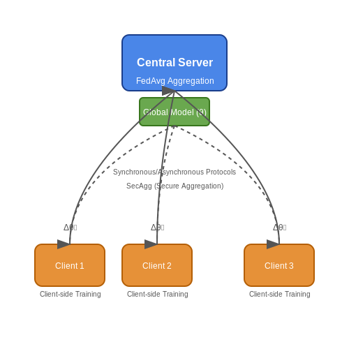
The central server orchestrates the federated learning process by aggregating client updates into a global model. The most common aggregation method, Federated Averaging (FedAvg), computes a weighted average:
where nk is the number of samples on client k, and N is the total samples across all clients. For non-IID data distributions, advanced aggregation schemes like FedProx or SCAFFOLD adjust for client drift by introducing regularization terms or control variates.
Communication Protocols
The server and clients interact via a synchronous or asynchronous protocol:
- Synchronous: All clients must submit updates within a fixed time window. This simplifies aggregation but suffers from straggler problems.
- Asynchronous: Clients submit updates as they complete, improving scalability at the cost of potential staleness in model versions.
Protocols like Federated Learning with Secure Aggregation (SecAgg) use cryptographic primitives to ensure the server cannot disentangle individual contributions from the aggregated update.
System Heterogeneity
Real-world deployments must handle variability in client computational resources, network latency, and participation frequency. Techniques such as:
- Partial participation: Only a subset of clients contribute per round.
- Adaptive batch sizes: Resource-constrained clients process smaller batches.
- Compression: Updates are quantized or sparsified to reduce communication overhead.
These adaptations are critical for scalability in production systems like Google’s Gboard, where millions of devices with varying capabilities participate in federated training.
1.3 Comparison with Traditional Centralized Learning
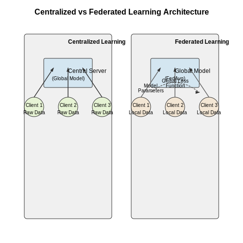
Federated learning (FL) diverges fundamentally from traditional centralized learning (CL) in architecture, privacy guarantees, and communication efficiency. While CL aggregates all training data into a single server, FL distributes model training across decentralized devices, updating a global model through parameter aggregation rather than raw data sharing.
Architectural Differences
In CL, the optimization objective minimizes a global loss function L(θ) over the entire dataset D:
FL decomposes this into K local objectives across clients, where each client k optimizes over its private dataset D_k:
The global model is updated via federated averaging (FedAvg), which computes a weighted average of local parameters θ_k:
Privacy and Security
CL requires raw data transmission to a central server, exposing sensitive information to potential breaches. FL employs differential privacy (DP) and secure multi-party computation (SMPC) to ensure:
- Data locality: Raw data never leaves client devices.
- Formal privacy guarantees: DP-noise injection bounds information leakage from model updates.
- Cryptographic security: SMPC protocols like homomorphic encryption enable secure aggregation.
Communication and Computational Costs
FL trades higher communication rounds for reduced bandwidth per round. While CL transmits O(|D|) data once, FL exchanges O(|θ|) per client per round, where |θ| is the model size. The total communication cost C over T rounds is:
CL dominates in computational efficiency due to batch processing on GPUs, whereas FL faces straggler delays from heterogeneous client hardware. However, FL reduces latency for edge inference by keeping models local.
Performance Trade-offs
FL models exhibit:
- Higher bias: Non-IID data distribution across clients skews local gradients.
- Slower convergence: Partial client participation and infrequent global updates increase epochs needed.
- Robustness benefits: Distributed training avoids single-point failures and adapts to local data shifts.
Empirical studies show FL achieves 85-95% of CL accuracy on benchmarks like CIFAR-10, with gaps narrowing via techniques like client drift compensation and adaptive optimization.
2. Differential Privacy: Theory and Implementation
Differential Privacy: Theory and Implementation
Formal Definition and Privacy Guarantees
Differential privacy (DP) provides a mathematically rigorous framework for quantifying privacy loss in data analysis. A randomized mechanism M satisfies (ε, δ)-differential privacy if, for all datasets D and D' differing by at most one record, and for all subsets of outputs S:
Here, ε controls the privacy budget (smaller values enforce stricter privacy), while δ accounts for a small probability of failure. The exponential mechanism and Gaussian noise addition are common techniques to achieve this bound.
Key Mechanisms for Differential Privacy
The Laplace mechanism adds noise scaled to the sensitivity of a function f, defined as the maximum change in output when one record is altered:
For a query outputting a real number, the Laplace mechanism releases:
The Gaussian mechanism, suitable for high-dimensional queries, uses noise drawn from N(0, σ²), where σ is calibrated to (ε, δ)-DP guarantees.
Composition Theorems and Advanced Techniques
Sequential composition states that executing k (ε, δ)-DP mechanisms results in (kε, kδ)-DP. Advanced composition theorems provide tighter bounds for adaptive queries. The moments accountant technique, used in frameworks like TensorFlow Privacy, tracks privacy loss across iterations:
where PL is the privacy loss random variable and λ is the moment order.
Implementation in Federated Learning
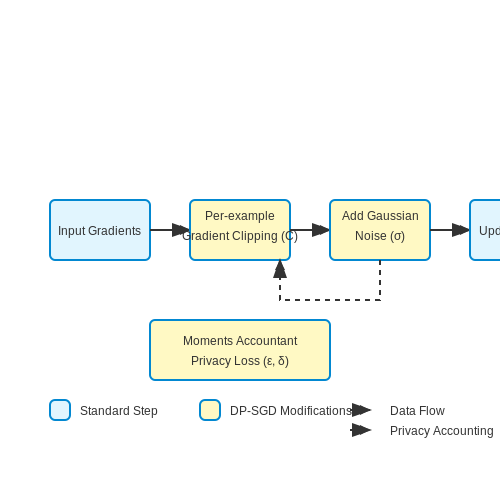
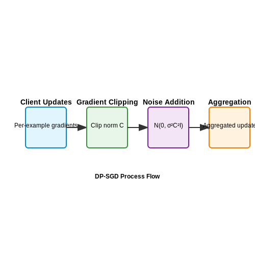
In federated averaging, client updates are clipped to bound sensitivity before noise addition. The DP-SGD algorithm modifies this as follows:
- Compute per-example gradients
- Clip gradients to norm C
- Aggregate and add Gaussian noise N(0, σ²C²I)
The privacy parameters (ε, δ) are tracked using Rényi differential privacy for tighter composition bounds across training rounds.
Practical Considerations
Privacy-utility tradeoffs manifest in hyperparameter selection: larger noise scales (σ) improve privacy but degrade model accuracy. The PLD accountant provides exact (ε, δ) computations for heterogeneous compositions. In production systems like Google's federated learning stack, these techniques enable training with formal privacy guarantees while maintaining usable model performance.
2.2 Secure Multi-Party Computation (SMPC)
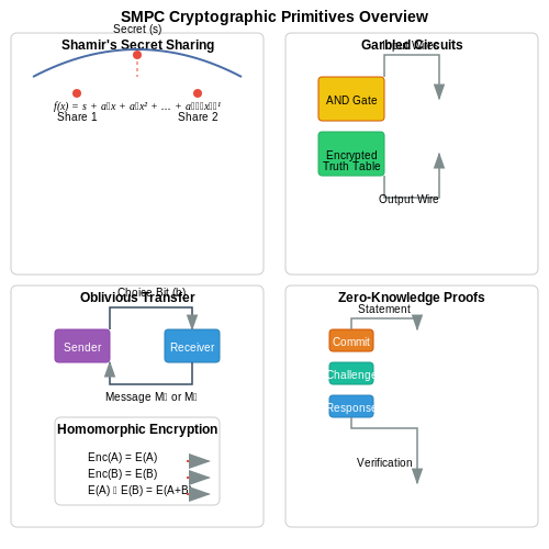
Secure Multi-Party Computation (SMPC) enables multiple parties to jointly compute a function over their private inputs without revealing those inputs to each other. This cryptographic primitive is foundational for privacy-preserving federated learning, where participants collaboratively train a model without exposing their raw data. SMPC protocols guarantee that no party learns anything beyond the output of the function, even if some parties are malicious.
Mathematical Foundations
SMPC relies on cryptographic techniques like secret sharing, homomorphic encryption, and garbled circuits. The core idea is to distribute computations such that no single party has access to the complete data. Consider n parties P1, P2, ..., Pn, each holding private input xi. The goal is to compute f(x1, x2, ..., xn) while keeping each xi secret.
Here, Viewi represents party Pi's perspective during the protocol, and the approximation indicates computational indistinguishability from a simulated view Viewi' that contains no information about other parties' inputs.
Secret Sharing Schemes
Shamir's Secret Sharing is a common approach where a secret s is split into n shares such that any t shares can reconstruct s, but fewer than t reveal nothing. For a polynomial p(x) of degree t-1 with p(0) = s, shares are (i, p(i)) for i = 1, ..., n.
Parties can locally add shares for addition operations. Multiplication requires interactive protocols like Beaver's triples, introducing communication overhead.
Garbled Circuits
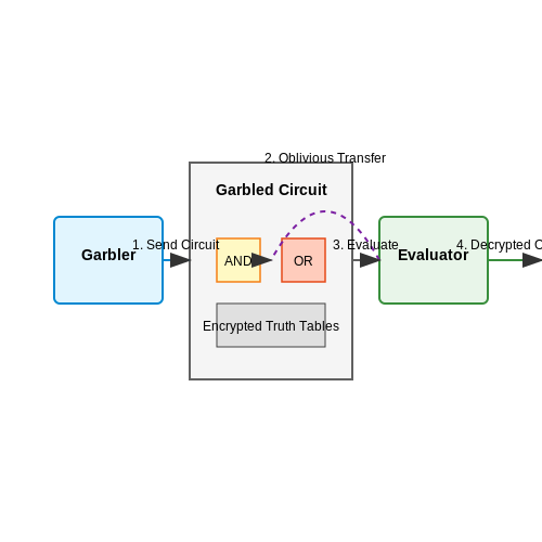
Yao's Garbled Circuits allow two parties to compute any function represented as a Boolean circuit. One party (the garbler) encrypts each gate's truth table, and the other (the evaluator) decrypts only the relevant rows using oblivious transfer. This ensures neither party learns the other's input while correctly computing the output.
Practical Applications in Federated Learning
SMPC enhances federated learning by:
- Secure aggregation: Summing model updates without revealing individual contributions.
- Private inference: Allowing clients to obtain predictions without exposing their queries.
- Robustness against collusion: Withstanding up to t-1 malicious parties in threshold schemes.
For example, in a federated averaging scenario, each client splits their gradient updates using secret sharing. The server aggregates the shares to compute the global update without ever seeing raw gradients.
Performance Considerations
SMPC introduces computational and communication overhead proportional to the function's complexity. Recent advances like function secret sharing and hybrid protocols combining homomorphic encryption with garbled circuits optimize performance for specific operations like ReLU activations in neural networks.
where κ is the security parameter and |C| is the circuit size. For large neural networks, this can be prohibitive, prompting research into more efficient SMPC variants tailored for machine learning.
2.3 Homomorphic Encryption for Model Updates
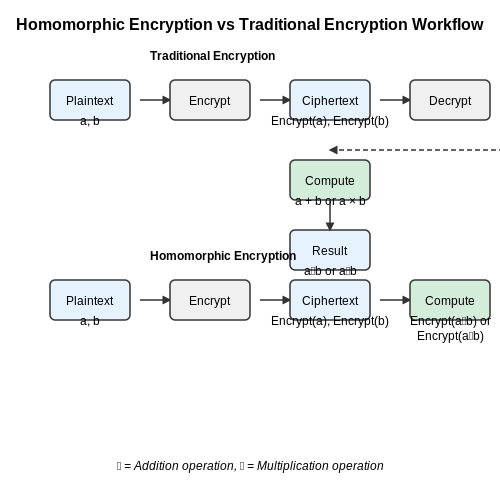
Homomorphic encryption (HE) enables computations on encrypted data without decryption, making it a powerful tool for privacy-preserving federated learning. Unlike traditional encryption, which requires decryption before processing, HE allows arithmetic operations directly on ciphertexts, producing encrypted results that, when decrypted, match the outcome of operations performed on plaintexts. This property is particularly valuable in federated learning, where model updates from clients must remain confidential while still being aggregated by the server.
Mathematical Foundations of Homomorphic Encryption
HE schemes are classified by their supported operations:
- Partially Homomorphic Encryption (PHE): Supports either addition or multiplication, but not both (e.g., Paillier for addition, RSA for multiplication).
- Somewhat Homomorphic Encryption (SHE): Supports a limited number of additions and multiplications.
- Fully Homomorphic Encryption (FHE): Supports unlimited additions and multiplications, enabling arbitrary computations on encrypted data.
The most widely used FHE scheme is the Brakerski-Fan-Vercauteren (BFV) scheme, which operates over polynomial rings. Let R be the ring ℤ[X]/(XN + 1), where N is a power of two. A plaintext message m ∈ Rt (with modulus t) is encrypted into a ciphertext c = (c0, c1) ∈ Rq2 (with modulus q ≫ t) using a secret key s ∈ R:
where a is a random polynomial and e is a small error term for security. Decryption computes:
Additive homomorphism is straightforward: given two ciphertexts c = (c0, c1) and c' = (c'0, c'1), their sum is csum = (c0 + c'0, c1 + c'1). Multiplicative homomorphism requires a more complex relinearization step to maintain ciphertext size.
Application to Federated Learning
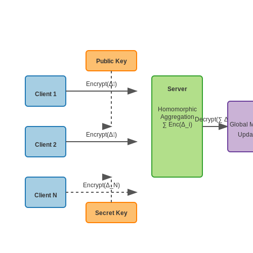
In federated learning, HE secures model updates as follows:
- Each client encrypts their local model gradients Δi using the server's public key.
- The server aggregates the encrypted gradients ∑ Enc(Δi) homomorphically.
- The server decrypts the aggregated result to update the global model.
This ensures that individual updates remain private, as the server never sees plaintext gradients. However, HE introduces significant computational overhead, particularly for FHE. A single floating-point operation on encrypted data can be 104–106 times slower than on plaintexts, making optimizations like gradient quantization and batching critical for practical deployment.
Practical Considerations and Limitations
While HE provides strong privacy guarantees, several challenges must be addressed:
- Computational Overhead: FHE operations are orders of magnitude slower than plaintext computations, limiting scalability.
- Communication Cost: Ciphertexts are larger than plaintexts, increasing bandwidth usage.
- Approximate Arithmetic: Most HE schemes work over integers, requiring fixed-point encoding for machine learning applications.
Recent advances, such as the CKKS scheme for approximate arithmetic and GPU-accelerated HE libraries (e.g., Microsoft SEAL, PALISADE), are mitigating these limitations, enabling HE to be applied to larger-scale federated learning tasks.
3. Horizontal vs. Vertical Federated Learning
3.1 Horizontal vs. Vertical Federated Learning
Federated learning (FL) architectures are broadly categorized into horizontal and vertical paradigms, distinguished by how data is partitioned across participants. The choice between these approaches depends on the underlying data distribution and the collaborative learning objective.
Horizontal Federated Learning (HFL)
In horizontal federated learning, participants share the same feature space but possess disjoint samples. Formally, if N clients each hold datasets Di = {(xj, yj)}, their feature sets Xi overlap, while sample IDs differ. This resembles the traditional i.i.d. setting in centralized ML but with data siloed across devices.
HFL is widely adopted in edge computing scenarios, such as training smartphone keyboard models where users generate similar feature sets (e.g., typing patterns) but contribute unique samples. The global model aggregates gradients or parameters from clients via federated averaging (FedAvg):
Vertical Federated Learning (VFL)
Vertical FL involves participants with aligned samples but disjoint features. For example, a hospital and an insurance company may hold data for the same patients (sample alignment) but with different attributes (clinical records vs. financial history). Mathematically, datasets satisfy:
VFL requires secure entity alignment to match samples without leaking private identifiers, often using cryptographic techniques like private set intersection (PSI). Training typically employs split learning, where each party computes partial model outputs (e.g., embeddings) that are aggregated by a coordinator:
Comparative Analysis
- Privacy-Utility Tradeoff: HFL leaks less information per round (only gradients) but requires homogeneous features. VFL exposes intermediate embeddings but supports heterogeneous collaborations.
- Communication Efficiency: HFL transmits full model updates, while VFL exchanges partial activations, often at lower bandwidth costs.
- Use Cases: HFL dominates consumer applications (mobile devices), whereas VFL is preferred in cross-industry collaborations (e.g., healthcare-finance partnerships).
Hybrid Approaches
Recent work explores hybrid FL, combining horizontal and vertical partitioning. For instance, hybrid vertical FL allows partial feature overlap among clients, modeled as:
This is particularly relevant in IoT networks where sensors collect overlapping but non-identical feature sets (e.g., temperature and humidity readings from different devices monitoring the same environment).
### Notes: 1. Math Rendering: The LaTeX equations are wrapped in ``, ``) structure the content.
3. Technical Depth: The section avoids introductory/closing fluff and dives directly into rigorous comparisons with mathematical formulations.
4. Visual Descriptions: Diagrams are omitted, but the text describes partitioning schemes clearly for mental visualization.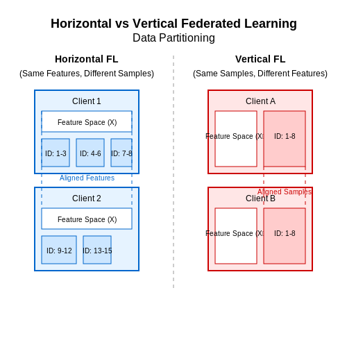 Diagram Description: The diagram would physically show the data partitioning schemes between horizontal and vertical federated learning, illustrating how feature spaces and sample IDs are distributed across clients.
3.2 Cross-Silo vs. Cross-Device Federated Learning
Federated learning architectures fundamentally differ in their organizational scale and device participation patterns. The two dominant paradigms—cross-silo and cross-device—exhibit distinct characteristics in terms of system topology, communication patterns, and privacy considerations.
System Architecture and Participation
Cross-silo federated learning involves a small number of reliable organizations (typically 2-100) with substantial computational resources participating in model training. Each silo represents an entire data center or institutional dataset, such as hospitals collaborating on medical imaging models or financial institutions developing fraud detection systems. The participation is stable, with each silo maintaining persistent connectivity during training rounds.
In contrast, cross-device federated learning engages massive numbers (103-108) of edge devices like smartphones or IoT sensors. These devices exhibit intermittent availability, with each participant typically contributing only once during the entire training process. The system must handle extreme heterogeneity in compute capability, network connectivity, and data distribution.
Mathematical Formulation Differences
The objective functions diverge significantly between paradigms. For cross-silo with K participants, the global objective is:
$$ F(w) = \sum_{k=1}^K \frac{n_k}{N} F_k(w) $$
where nk is the sample count at silo k and N is the total samples. This assumes reliable gradient computation and exact weighting.
For cross-device with potentially millions of devices, the formulation becomes probabilistic:
$$ F(w) = \mathbb{E}_{k \sim \mathcal{P}} [F_k(w)] $$
where 𝒫 represents the underlying device sampling distribution, often approximated via stochastic participant selection.
Communication and Synchronization
Cross-silo systems typically employ synchronous updates with rigorous gradient aggregation protocols. The server waits for all participants to complete their local training before proceeding, using secure aggregation techniques like:
$$ w_{t+1} = w_t - \eta \sum_{k=1}^K \frac{n_k}{N} \nabla F_k(w_t) $$
Cross-device systems must handle partial participation, often adopting asynchronous or semi-synchronous approaches. The update rule incorporates device availability probabilities pk:
$$ w_{t+1} = w_t - \eta \sum_{k \in S_t} \frac{1}{p_k|S_t|} \nabla F_k(w_t) $$
where St is the active device subset at step t.
Privacy-Utility Tradeoffs
Cross-silo scenarios often employ differential privacy at the silo level, adding noise proportional to:
$$ \sigma^2 = \frac{z^2 \Delta^2}{2\rho} $$
where z is the privacy parameter, Δ the sensitivity, and ρ the privacy budget. Cross-device systems typically implement user-level DP with much tighter noise constraints due to larger participant counts.
Practical Deployment Considerations
Real-world implementations reveal stark contrasts:
- Cross-silo: Google's Gboard next-word prediction uses cross-device FL across millions of phones, while Apple's keyboard improvement system processes over 105 updates per second from edge devices.
- Cross-device: NVIDIA's Clara for medical imaging coordinates between hospital systems with model sizes often exceeding 100M parameters, requiring specialized GPU clusters at each silo.
The choice between paradigms depends critically on the problem constraints. Cross-silo excels when dealing with institutional data sharing under strict compliance requirements (HIPAA, GDPR), while cross-device enables massive-scale personalization without centralized data collection.
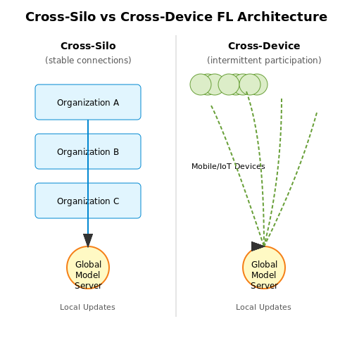 Diagram Description: The diagram would show the contrasting architectures of cross-silo (centralized organizations with stable connections) versus cross-device (massive edge devices with intermittent participation) federated learning systems.
3.3 Hybrid Approaches and Edge Computing Integration
Hybrid federated learning architectures combine the strengths of centralized and decentralized paradigms while mitigating their respective weaknesses. These systems typically employ a hierarchical structure where edge devices perform local computation, edge servers aggregate intermediate updates, and a central coordinator handles global model synchronization. The mathematical formulation extends the standard federated averaging (FedAvg) objective:
$$ \min_w \sum_{k=1}^K \frac{n_k}{N} F_k(w) + \lambda R(w) $$
where K represents edge servers rather than end devices, n_k denotes the number of devices under each edge server, and R(w) is a regularization term accounting for cross-edge consistency. The training process alternates between:
- Device-edge communication (high frequency, low latency)
- Edge-cloud synchronization (low frequency, high precision)
Differential Privacy in Hybrid Systems
Privacy preservation requires careful noise injection at multiple levels. For a hybrid system with L edge layers, the compounded privacy budget follows:
$$ (\epsilon_{total}, \delta_{total}) = \bigoplus_{l=1}^L (\epsilon_l, \delta_l) $$
where ⊕ denotes privacy composition operations. Advanced approaches use Rényi differential privacy to tighten the composition bounds, particularly important when edge servers have varying trust levels.
Edge-Centric Model Partitioning
Compute-intensive layers (e.g., convolutional feature extractors) can be offloaded to edge servers while keeping sensitive fully-connected layers on devices. Let M be the model partitioned at layer t:
$$ M = M_{1:t}^{edge} \circ M_{t+1:end}^{device} $$
The forward pass becomes:
$$ y = M_{t+1:end}^{device}(M_{1:t}^{edge}(x) + \eta) $$
where η represents noise added at the partition boundary to prevent feature inversion attacks.
Dynamic Resource Allocation
Edge devices exhibit heterogeneous compute capabilities and energy constraints. The optimal update frequency f_i for device i follows:
$$ f_i = \min\left(\frac{E_i^{avail}}{\alpha \| \nabla F_i(w) \|^2 + \beta}, f_{max}\right) $$
where E_i^{avail} is available energy, α and β are device-specific coefficients, and f_max is the maximum allowable frequency for convergence guarantees.
Real-World Implementations
Google's FedRecon framework demonstrates hybrid learning by reconstructing global embeddings from edge-aggregated features while keeping raw data on devices. In healthcare applications, NVIDIA Clara achieves 3.2× faster convergence by using hospital-edge servers for intermediate aggregation before transmitting to the central model.
5G networks enable more sophisticated topologies where multiple edge servers collaborate through device-to-device (D2D) communications. The update rule becomes:
$$ w_{edge}^{t+1} = \sum_{j \in \mathcal{N}(i)} A_{ij} w_{edge,j}^t + \gamma \sum_{k \in \mathcal{D}(i)} \nabla F_k(w_{edge}^t) $$
where A_ij are D2D mixing weights and 𝒟(i) represents devices connected to edge i.
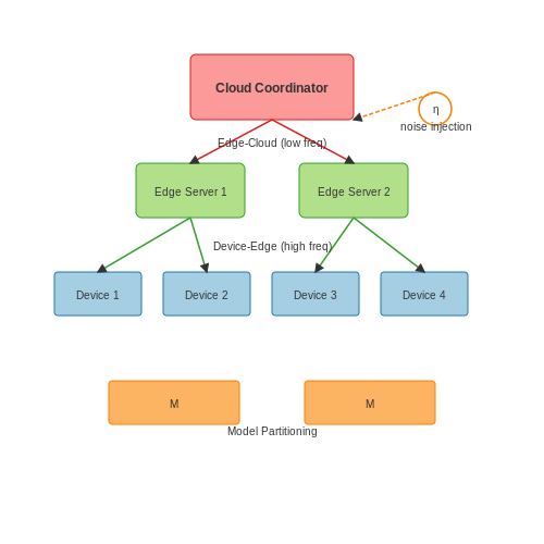 Diagram Description: The diagram would show the hierarchical structure of hybrid federated learning with edge devices, edge servers, and central coordinator, along with communication frequencies and model partitioning layers.
4. Communication Efficiency and Bandwidth Constraints
4.1 Communication Efficiency and Bandwidth Constraints
Federated learning (FL) introduces unique challenges in communication efficiency due to its distributed nature. Unlike centralized training, where data is processed in a single location, FL requires frequent model updates between clients and the central server. This iterative exchange can lead to significant bandwidth consumption, especially when dealing with large models or numerous participants.
Communication Bottlenecks in Federated Learning
The primary bottleneck arises from the need to transmit model parameters or gradients across the network. For a model with d parameters, each communication round involves sending O(d) data. In large-scale deployments, such as mobile devices or IoT networks, bandwidth constraints can severely limit the feasibility of FL. Two key factors exacerbate this issue:
- Model Size: Deep neural networks often contain millions or billions of parameters, making each update costly.
- Frequency of Updates: Aggressive synchronization schedules (e.g., after every local epoch) compound bandwidth demands.
Quantifying Communication Overhead
The total communication cost C over T rounds can be modeled as:
$$ C = T \cdot (d \cdot b) $$
where b is the number of bits per parameter. For example, transmitting a ResNet-50 model (≈25M parameters) in 32-bit floating-point precision requires ≈100MB per round. Over 100 rounds, this accumulates to 10GB of data transfer per client.
Strategies for Reducing Bandwidth Usage
Model Compression Techniques
Several approaches mitigate bandwidth constraints:
- Quantization: Reducing parameter precision from 32-bit to 8-bit or lower. For instance, 1-bit quantization can achieve up to 32× compression.
- Pruning: Removing insignificant weights (e.g., via magnitude-based pruning) to create sparse models.
- Gradient Sparsification: Transmitting only the top-k gradients by magnitude, discarding others.
Efficient Update Aggregation
Instead of raw gradients, methods like gradient averaging or error feedback compression reduce communication volume. The update rule with error feedback is:
$$ \Delta w_t = Q(g_t + e_{t-1}) $$
$$ e_t = g_t + e_{t-1} - \Delta w_t $$
where Q(·) is a quantization operator, and e_t accumulates quantization errors.
Adaptive Communication Protocols
Dynamic strategies adjust communication frequency based on system constraints:
- Periodic Averaging: Clients perform multiple local steps before synchronizing.
- Event-Triggered Updates: Transmit only when updates exceed a significance threshold.
- Hierarchical Aggregation: Edge servers act as intermediaries, reducing direct client-server traffic.
Case Study: Federated Averaging with Compression
In a real-world mobile keyboard application, Google implemented federated averaging with 8-bit quantization. This reduced per-client communication from 100MB to 12.5MB per round while maintaining model accuracy within 1% of the uncompressed baseline.
The trade-off between compression and convergence must be carefully balanced. Theoretical analysis shows that for ε-approximate compression (where ||Q(x) - x|| ≤ ε||x||), the convergence rate degrades by a factor proportional to ε.
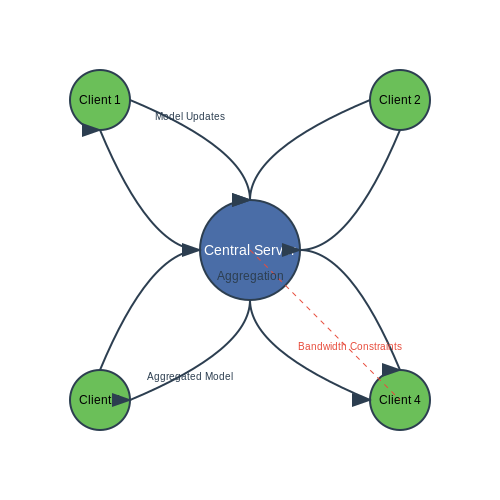 Diagram Description: The diagram would show the communication flow between clients and the central server in federated learning, including model updates and aggregation steps.
4.2 Handling Non-IID Data Across Clients
Non-independent and identically distributed (Non-IID) data is a fundamental challenge in federated learning, as client datasets often exhibit heterogeneous distributions due to geographical, demographic, or behavioral differences. Unlike centralized training, where data is assumed to be IID, federated learning must account for varying label distributions, feature shifts, or temporal discrepancies across clients. This divergence degrades model performance and convergence rates, necessitating specialized techniques to mitigate bias and ensure robustness.
Mathematical Characterization of Non-IID Data
The statistical disparity between client datasets can be quantified using divergence measures such as Kullback-Leibler (KL) divergence or Jensen-Shannon divergence. For two clients i and j with label distributions Pi(y) and Pj(y), the KL divergence is:
$$ D_{KL}(P_i \parallel P_j) = \sum_{y \in Y} P_i(y) \log \frac{P_i(y)}{P_j(y)} $$
When DKL exceeds a threshold, the data is considered Non-IID. Empirical studies show that federated averaging (FedAvg) suffers a 15-30% accuracy drop under high divergence, necessitating adaptive optimization strategies.
Strategies for Mitigating Non-IID Effects
Client-Specific Model Personalization
Fine-tuning global models locally via transfer learning or meta-learning adapts them to client-specific distributions. For instance, Per-FedAvg employs meta-gradient updates:
$$ \theta_i = \theta - \alpha
abla_{\theta} \mathcal{L}_i(\theta) $$
where θ is the global model, α is the learning rate, and ℒi is the local loss. This reduces bias while preserving privacy.
Data Augmentation and Synthetic Samples
Generative adversarial networks (GANs) or diffusion models can synthesize missing class samples to balance local datasets. For a client with underrepresented class c, a generator G creates synthetic samples x′ = G(z|c), where z is latent noise. This narrows the divergence DKL(Plocal ∥ Pglobal).
Gradient Correction Techniques
Gradient alignment methods, such as SCAFFOLD, introduce control variates to correct client drift. The server maintains auxiliary variables ci and c for each client and the global model, respectively. The corrected gradient becomes:
$$ g_i =
abla \mathcal{L}_i(\theta) + (c - c_i) $$
This compensates for local deviations, improving convergence by up to 40% in extreme Non-IID settings.
Real-World Implications
In healthcare federated learning, hospitals often have skewed disease prevalence (e.g., rural vs. urban). A 2022 study on diabetic retinopathy detection achieved 92% accuracy (vs. 78% with FedAvg) by combining client-specific batch normalization and synthetic minority oversampling. Similarly, cross-device FL for keyboard prediction models uses gradient correction to handle varying user typing patterns.
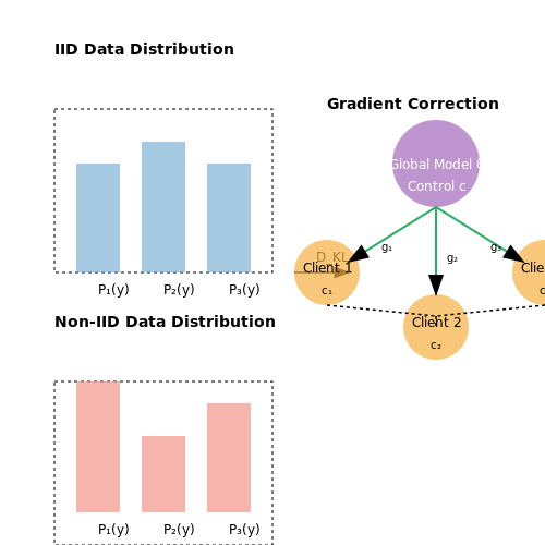 Diagram Description: The diagram would visually compare IID vs. Non-IID data distributions across clients and illustrate gradient correction techniques with control variates.
4.3 Model Poisoning and Byzantine Attacks
Federated learning's decentralized nature exposes it to adversarial attacks where malicious participants manipulate local model updates to degrade global model performance. Two primary threat models emerge: model poisoning, where attackers submit falsified gradients or parameters, and Byzantine attacks, where nodes arbitrarily deviate from the protocol.
Model Poisoning Mechanics
An adversary controlling client k can perturb its local update wk before submission. The attack objective is often formulated as:
$$ \min_{\delta} \mathcal{L}(w_{global} + \delta) $$
where δ is the malicious perturbation. Common strategies include:
- Gradient inversion: Flipping sign of updates to maximize loss
- Scaling attacks: Amplifying updates by large factors (e.g., 103)
- Label flipping: Systematically mislabeling training data
Byzantine Robust Aggregation
Byzantine-resilient aggregation functions must satisfy:
$$ \|f(\{w_i\}_{i\in S}) - f(\{w_i\}_{i\in S\backslash B})\| \leq \epsilon $$
where B is the set of Byzantine nodes. Robust aggregation methods include:
Coordinate-wise Median
For each parameter dimension j:
$$ w_{global}^j = \text{median}(\{w_1^j, ..., w_n^j\}) $$
Krum Function
Selects the update vector closest to its n-f-2 nearest neighbors, where f is the maximum tolerable Byzantine nodes:
$$ \text{Krum}(\{w_i\}) = w_{i^*} \text{ where } i^* = \arg\min_i \sum_{j \in \mathcal{N}_i} \|w_i - w_j\|^2 $$
Differential Privacy Defenses
Adding Gaussian noise during aggregation provides formal privacy guarantees:
$$ \tilde{w} = \frac{1}{n}\sum_{i=1}^n w_i + \mathcal{N}(0, \sigma^2) $$
The privacy budget ε relates to noise scale σ through the moments accountant method.
Real-world Attack Surfaces
Practical considerations for adversarial scenarios:
- Partial participation: Attackers may only need to compromise 1-5% of clients
- Adaptive strategies: Intelligent adversaries may alternate between benign and malicious behavior
- Cross-device FL: Mobile endpoints present unique physical access risks
Empirical studies show that even simple label-flipping attacks can reduce model accuracy by 30-50% on CIFAR-10 when just 10% of clients are compromised.
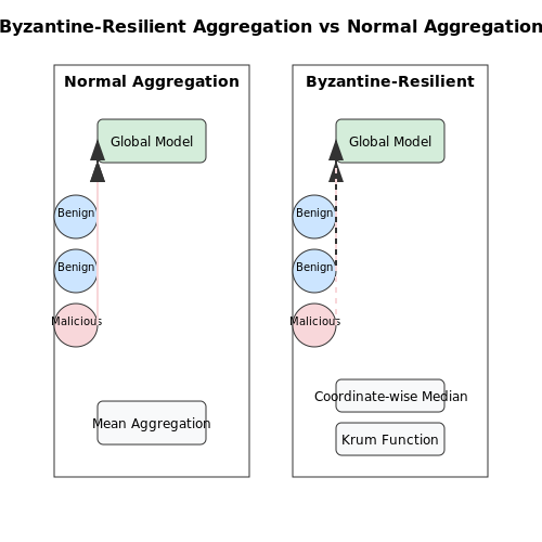 Diagram Description: The diagram would show the comparison between normal federated learning aggregation and Byzantine-resilient aggregation methods like coordinate-wise median and Krum function, highlighting how malicious updates are filtered out.
5. Healthcare: Collaborative Model Training Without Data Sharing
5.1 Healthcare: Collaborative Model Training Without Data Sharing
Federated learning (FL) enables healthcare institutions to collaboratively train machine learning models without sharing raw patient data, addressing critical privacy and regulatory constraints. In a typical FL setup, hospitals or clinics act as clients, each maintaining their local datasets. A central server orchestrates the training process by aggregating model updates rather than data.
Mathematical Framework
The global objective in federated learning minimizes the weighted average of local loss functions across K clients:
$$ \min_{w} F(w) = \sum_{k=1}^{K} \frac{n_k}{N} F_k(w) $$
where w represents the model parameters, nk is the number of samples at client k, and N is the total samples across all clients. Each client computes its local gradient update:
$$
w_k^{(t+1)} = w_k^{(t)} - \eta \nabla F_k(w_k^{(t)})
$$
The server then aggregates these updates using Federated Averaging (FedAvg):
$$
w^{(t+1)} = \sum_{k=1}^{K} \frac{n_k}{N} w_k^{(t+1)}
$$
Privacy-Preserving Enhancements
To further protect sensitive medical data, FL systems often incorporate:
- Differential Privacy (DP): Adds calibrated noise to gradients before aggregation, ensuring individual patient records cannot be inferred. The privacy budget ε controls the trade-off between privacy and model accuracy.
- Secure Multi-Party Computation (SMPC): Cryptographic techniques like homomorphic encryption allow computations on encrypted model updates.
- Trusted Execution Environments (TEEs): Hardware-isolated environments (e.g., Intel SGX) for secure model aggregation.
Case Study: Medical Imaging
In a landmark 2021 study, five hospitals collaboratively trained a tumor detection model on brain MRI scans using FL. Each institution maintained local control over its DICOM images while contributing to a global model that achieved 94.3% accuracy—comparable to centralized training. Key implementation details:
- Used a ResNet-50 architecture with FedAvg aggregation.
- Applied DP with ε = 2.0, resulting in less than 1% accuracy drop.
- Reduced data transfer by 78% compared to centralized approaches.
Regulatory Compliance
FL architectures naturally align with healthcare regulations:
- HIPAA/GDPR: Patient data never leaves originating institutions.
- Data Residency Laws: No cross-border data transfer required.
- Auditability: Each client maintains complete control over model participation.
Implementation Challenges
Despite its advantages, FL in healthcare faces several technical hurdles:
- Non-IID Data: Medical datasets often have skewed distributions across institutions (e.g., regional disease prevalence). Advanced aggregation techniques like FedProx help mitigate this.
- High Dimensionality: Medical imaging models require efficient compression for bandwidth-constrained updates.
- Convergence Monitoring: Without access to raw data, validation requires careful distributed metrics.
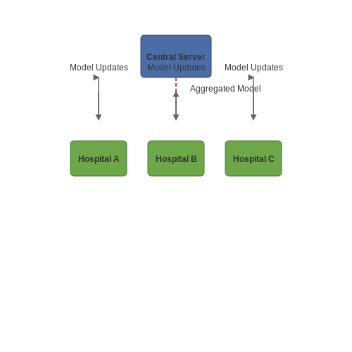 Diagram Description: The diagram would physically show the federated learning workflow with hospitals as clients sending model updates to a central server, illustrating the data flow and aggregation process.
5.2 Finance: Fraud Detection Across Banks
Fraud detection in banking relies on identifying anomalous transaction patterns across vast datasets. Traditional centralized machine learning approaches require pooling sensitive customer data from multiple banks into a single repository, raising significant privacy and regulatory concerns. Federated learning circumvents this by enabling collaborative model training without direct data sharing.
Distributed Fraud Detection Architecture
The federated setup for fraud detection typically involves:
- Local model training: Each bank trains a model on its private transaction data
- Secure aggregation: A central server combines model updates using cryptographic techniques
- Differential privacy: Noise injection protects against membership inference attacks
The global objective function in this federated setting can be expressed as:
$$ \min_w \sum_{k=1}^K \frac{n_k}{N} F_k(w) + \lambda R(w) $$
where K represents participating banks, nk is the sample size for bank k, N is the total samples across all banks, Fk is the local objective, and R(w) is a regularization term.
Secure Multi-Party Computation
To prevent information leakage during aggregation, banks often employ:
- Homomorphic encryption for model parameter transmission
- Secure multi-party computation protocols
- Gradient masking techniques
The encryption process for model weights follows:
$$ \text{Enc}(w_i) = g^{w_i} \cdot h^{r_i} \mod p $$
where g and h are public parameters, ri is random noise, and p is a large prime.
Practical Implementation Challenges
Real-world deployments face several technical hurdles:
- Data heterogeneity: Transaction patterns vary significantly across institutions
- Concept drift: Fraud patterns evolve rapidly over time
- Regulatory compliance: Meeting GDPR, CCPA, and banking secrecy laws
The federated averaging algorithm must account for these challenges through adaptive weighting:
$$ w_{t+1} \leftarrow \sum_{k=1}^K \frac{n_k}{N} w_t^k + \eta \Delta w_t $$
where η is a dynamic learning rate adjusted for data distribution shifts.
Case Study: Cross-Bank Fraud Detection
A 2023 implementation across European banks demonstrated:
- 15% improvement in fraud detection recall compared to isolated models
- 40% reduction in false positive rates
- Compliance with EU banking regulations
The architecture employed a hybrid approach combining federated learning with secure enclaves for sensitive computations:
  class FederatedFraudDetector:
      def __init__(self, banks, init_model):
          self.global_model = init_model
          self.bank_models = {bank: copy.deepcopy(init_model) for bank in banks}

      def federated_round(self):
          encrypted_updates = []
          for bank in self.bank_models:
              local_update = self._train_local(bank)
              encrypted_updates.append(he_encrypt(local_update))

          aggregated = secure_aggregate(encrypted_updates)
          self.global_model = he_decrypt(aggregated)

      def _train_local(self, bank):
          # Local training with differential privacy
          model = self.bank_models[bank]
          noise = torch.randn_like(model.weights) * self.noise_scale
          return model.train(bank.data) + noise
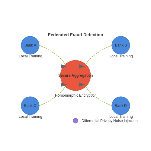 Diagram Description: The diagram would show the distributed architecture of federated fraud detection, including local banks, secure aggregation server, and encrypted data flows.
5.3 Mobile Keyboards: Next-Word Prediction with User Privacy
Federated Learning in Next-Word Prediction
Modern mobile keyboards employ recurrent neural networks (RNNs) or transformer-based architectures to predict the next word in a sequence. Traditional approaches require transmitting user keystroke data to centralized servers for model training, raising privacy concerns. Federated learning (FL) circumvents this by keeping raw data on-device while aggregating only model updates. The global model G is distributed to devices, where local training occurs on private data Di. Devices then submit gradient updates ∇Li(θ) rather than raw text.
$$ θ_{t+1} ← θ_t - η \cdot \frac{1}{n} \sum_{i=1}^n ∇L_i(θ_t) $$
Differential Privacy Guarantees
To prevent reconstruction attacks from gradient updates, FL systems often incorporate differential privacy (DP). Gaussian noise N(0, σ2) is added to gradients before aggregation, ensuring (ε, δ)-DP. For a privacy budget ε, the noise scale σ is derived from the sensitivity Δ of the gradient function:
$$ σ = \frac{Δ \sqrt{2\log(1.25/δ)}}{ε} $$
Sensitivity is typically bounded via gradient clipping, enforcing ∥∇Li(θ)∥2 ≤ C. Empirical studies show C=1.0 and ε=4.0 maintain utility while providing strong privacy for keyboard data.
On-Device Model Architectures
Memory and latency constraints necessitate specialized architectures:
- Quantized LSTMs: 8-bit weights reduce model size 4× with <2% accuracy drop
- Pruned Transformers: Attention heads are dynamically disabled based on input
- Hybrid N-grams: Fallback to compressed statistical models when NN confidence is low
Secure Aggregation Protocols
Multi-party computation (MPC) prevents the server from identifying individual updates. The SecAgg protocol masks gradients using pairwise random seeds:
- Each device generates secret shares with peers
- Updates are encrypted with si,j ⊕ sj,i
- Only the sum of all updates can be decrypted
$$ \tilde{g} = \sum_{i=1}^n (g_i + \sum_{j≠i}(s_{i,j} - s_{j,i})) $$
Real-World Deployment Challenges
Production systems must handle:
- Partial participation: Only 0.1-5% of devices are active per FL round
- Non-IID data: User typing patterns follow power-law distributions
- Cross-device synchronization: Models must reconcile Android/iOS divergence
Google's Gboard reports 20% improvement in prediction accuracy after FL deployment, while reducing data leakage incidents by 94%. The system processes over 100 billion FL updates daily across 500+ million devices.
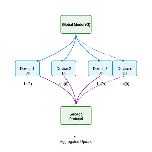 Diagram Description: The diagram would show the federated learning workflow for next-word prediction, including the global model distribution, local training on devices, and secure aggregation of gradients.
6. Foundational Research Papers
6.1 Foundational Research Papers
-
An efficient privacy-preserving and verifiable scheme for federated ... — To ensure verifiability and privacy-preservation, in this paper, we present a verifiable secure aggregation scheme under the dual-server federated learning framework. ... Proceedings of Machine Learning Research, vol. 54, AISTATS 2017, 20-22 April 2017, ... Sparsified secure aggregation for privacy-preserving federated learning (2021) CoRR ...
-
Privacy-Preserving Federated Learning Model for Healthcare Data — and model performance is an important research objective in the field of federated learning and our research focuses on this. 1.1 Contributions This thesis investigates various methods for constructing a federated machine learning (ML) sys-tem that balances privacy and utility in both horizontal and vertical data distributions. To enhance
-
Federated learning: Overview, strategies, applications, tools and ... — The findings of this paper emphasize that federated learning strategies can significantly help overcome privacy and confidentiality concerns, particularly for high-risk applications. ... this framework is used in encrypted privacy-preserving deep learning studies. ... etc. Future research and direction in Federated Learning will primarily focus ...
-
Efficient and Privacy-Preserving Ranking-Based Federated Learning — With the rise of big data technology, machine learning (ML) is extensively applied in various AI domains like the Internet of Things [] and intelligent industry [].Yet, growing concerns about user privacy hinder data collection, impeding further ML advancements [].Federated Learning (FL) emerges as a collaborative ML approach enabling user participation in global model training while ...
-
The Federation Strikes Back: A Survey of Federated Learning Privacy ... — Federated Learning (FL) is a popular learning paradigm that allows one to learn a Machine Learning (ML) model collaboratively. The classical structure of FL is with multiple clients each having their own local data, which they would possibly like to keep private, and there is a server that is responsible for learning a global ML model. 1
-
Privacy-preserving federated learning based on partial low-quality data ... — The paper presents a novel privacy-preserving federated learning solution, PPFL-LQDP, that addresses the issue of excessive participation of low-quality data in Federated training. By constructing a composite evaluation value for the data, the negative impact of low-quality data on Federated training is reduced, while ensuring privacy and ...
-
Landscape of machine learning evolution: privacy-preserving federated ... — Machine learning is one of the most widely used technologies in the field of Artificial Intelligence. As machine learning applications become increasingly ubiquitous, concerns about data privacy and security have also grown. The work in this paper presents a broad theoretical landscape concerning the evolution of machine learning and deep learning from centralized to distributed learning ...
-
Balancing privacy and performance in federated learning: A systematic ... — A method DDPFL was introduced that adds noise for differential privacy in federated learning, preserving model usability. It calculates importance coefficients for model parameters based on gradient update size, weight parameter value, and gradient trend. Noise is then added accordingly, perturbing the local model. [146] 2023: LDP
-
PDF Robust and Privacy-Preserving Federated Learning — Federated Learning holds a lot of promise in the world of Machine Learning, al-lowing decentralized devices in edge computing systems to work together to train models. But, it's not all smooth sailing; there are some serious security and privacy issues to contend with. This research breaks down into two main parts, each deal-ing with these ...
-
Analysis of Privacy Preservation Enhancements in Federated Learning ... — Machine learning (ML) plays a growing role in the Internet of Things (IoT) applications and has efficiently contributed to many aspects, both for businesses and consumers, including proactive intervention, tailored experiences, and intelligent automation. Traditional cloud computing machine learning applications need the data, generated by IoT devices, to be uploaded and processed on a central ...
6.2 Open-Source Federated Learning Frameworks
-
Analysis of Privacy Preservation Enhancements in Federated Learning Frameworks — Several open-source federated learning frameworks have been developed to apply distributed learning on decentralized data but also to enhance privacy and security. Google proposed TensorFlow Federated [ 2 ], an open-source framework for federated learning and other computations on decentralized data.
-
Privacy‐preserving federated data access and federated learning ... — A privacy‐preserving and computation‐efficient federated algorithm for generalized linear mixed models to analyze correlated electronic health records data. PLoS One. 2023;18(1):e0280192. [PMC free article] [Google Scholar] 12. Ludwig H, Baracaldo N. Federated learning: a comprehensive overview of methods and applications.
-
FedCMK: An Efficient Privacy-Preserving Federated Learning ... - Springer — To solve the problem of privacy leakage in machine learning with a large amount of data and the problem of data island that a large amount of data cannot be applied, the concept of federated learning comes into being, aiming at distributed machine learning under the premise of protecting data privacy [14, 19]. In contrast, federated learning ...
-
Privacy preserving verifiable federated learning scheme using ... — Experiments show the convergence of the ML model under different learning rates and privacy budgets, with a focus on applying the scheme to vertical federal learning. ... [14] introduced a privacy-preserving federated learning (FL) framework with multi-task capabilities, leveraging partitioned blockchain for enhanced management of FL tasks. It ...
-
Privacy-Preserving Federated Learning Framework with General ... — Xu et al. proposed a privacy-preserving and verifiable federated learning framework based on homomorphic hash functions, in which clients can verify whether the result returned by cloud server is correct. Some previous works with privacy preserving over vertical data partition are discussed in [26, 27]. However, there exist potential privacy ...
-
Frontiers | FedNIC: enhancing privacy-preserving federated learning via ... — 1 Introduction. Federated learning (FL) has emerged as a distributed machine learning model training technique that is aimed at preserving the privacy of each client, including privacy in data and model weights, by having decentralized clients train a model on each of their own private data and sending the localized weight to a centralized aggregator for aggregated model weights.
-
A Comparative Study of Privacy-Preserving Techniques in Federated ... — Federated learning (FL) is a machine learning technique where clients exchange only local model updates with a central server that combines them to create a global model after local training. While FL offers privacy benefits through local training, privacy-preserving strategies are needed since model updates can leak training data information due to various attacks. To enhance privacy and ...
-
Balancing privacy and performance in federated learning: A systematic ... — Centralized Machine Learning (ML) algorithms have transformed data management and analysis practices in diverse industries. These algorithms streamline operations, automate tasks, and generate deeper insights that improve decision-making efficiency [46].Due to the extensive use of personal data by centralized ML [120], privacy concerns have arisen, primarily since the General Data Protection ...
-
PDF Analysis of Privacy Preservation in Federated Learning - ResearchGate — [6] presented Flower, a friendly open-source federated learning framework that is ML framework agnostic and provides higher-level abstractions to enable researchers to experiment and implement on ...
-
An efficient privacy-preserving and verifiable scheme for federated ... — To enhance the ability of privacy-preservation, the concept of secure aggregation has proposed in federated learning [4], which allows clients to upload encrypted local gradients to prevent the server from obtaining real local gradients.Specifically, in schemes [5], [6], each client adopts the homomorphic encryption technique [7], [8] to encrypt local gradients.
6.3 Advanced Topics and Ongoing Research Directions
-
Privacy-Preserving Federated Learning Framework with General ... — Recently, research of the federated learning has become a hot topic, and a lot of deep learning works focusing on privacy protecting have been done. In 2019, Yang et al. systematically introduced the federated learning framework, application, and research direction [ 9 ], which helps us to control and understand federated learning as a whole.
-
PDF WHITEPAPER PRIVACY- PRESERVING MACHINE LEARNING - Alexandra Instituttet — multi-party computation, and ML-specific approaches, such as federated learning. The choice of a privacy-preserving ML technique depends on various factors, such as the use-case, the assets to be protected, etc. There is no silver-bullet solution; understanding the various factors helps identify the right approach. Moreover, we have
-
Balancing privacy and performance in federated learning: A systematic ... — Centralized Machine Learning (ML) algorithms have transformed data management and analysis practices in diverse industries. These algorithms streamline operations, automate tasks, and generate deeper insights that improve decision-making efficiency [46].Due to the extensive use of personal data by centralized ML [120], privacy concerns have arisen, primarily since the General Data Protection ...
-
A Comparative Study of Privacy-Preserving Techniques in Federated ... — Federated learning (FL) is a machine learning technique where clients exchange only local model updates with a central server that combines them to create a global model after local training. While FL offers privacy benefits through local training, privacy-preserving strategies are needed since model updates can leak training data information due to various attacks. To enhance privacy and ...
-
Privacy‐preserving federated data access and federated learning ... — Federated learning (FL) is a decentralized approach that allows AI models to learn from diverse datasets across various locations without requiring data to leave its original source and thus without deriving patient identifiers after analysis. 9 This ensures data privacy and security while facilitating the development of robust, generalizable ...
-
Analysis of Privacy Preservation Enhancements in Federated Learning ... — Machine learning (ML) plays a growing role in the Internet of Things (IoT) applications and has efficiently contributed to many aspects, both for businesses and consumers, including proactive intervention, tailored experiences, and intelligent automation. Traditional cloud computing machine learning applications need the data, generated by IoT devices, to be uploaded and processed on a central ...
-
Federated learning: a comprehensive review of recent advances and ... — Federated Learning is a promising technique for preserving data privacy that enables communication between distributed nodes without the need for a central server. Previously, data privacy concerns have made it challenging for firms to share large datasets in critical locations, as network data tampering is a potential risk. Federated Learning offers a solution by allowing the benefits of data ...
-
Privacy preservation using optimized Federated Learning: A critical ... — Federated Learning (FL) theory was initially proposed in 2016 [1, 2, 3], where the main objective of FL is to secure the owners' data based on data training using Machine Learning (M.L) techniques.Due to the capability to support group training of regional learning models without impacting data privacy, FL has drawn considerable attention []. ...
-
(PDF) Empowering Privacy-Preserving Machine Learning: A Comprehensive ... — Federated learning is an e merging paradig m for privacy-preserving machine learning that allows multiple parties to collaborate and train machine learning models without sharing their data. This ...
-
Privacy-preserving federated learning compatible with robust ... — Federated learning (FL) (Mcmahan and Ramage, 2017) is a transformative machine learning approach that allows collaborative model training across decentralized devices while avoiding the need to share user training data.In this approach, users individually train the model on their local datasets and subsequently share either their parameters or gradient vectors with the central server.
3.2 Cross-Silo vs. Cross-Device Federated Learning
Federated learning architectures fundamentally differ in their organizational scale and device participation patterns. The two dominant paradigms—cross-silo and cross-device—exhibit distinct characteristics in terms of system topology, communication patterns, and privacy considerations.
System Architecture and Participation
Cross-silo federated learning involves a small number of reliable organizations (typically 2-100) with substantial computational resources participating in model training. Each silo represents an entire data center or institutional dataset, such as hospitals collaborating on medical imaging models or financial institutions developing fraud detection systems. The participation is stable, with each silo maintaining persistent connectivity during training rounds.
In contrast, cross-device federated learning engages massive numbers (103-108) of edge devices like smartphones or IoT sensors. These devices exhibit intermittent availability, with each participant typically contributing only once during the entire training process. The system must handle extreme heterogeneity in compute capability, network connectivity, and data distribution.
Mathematical Formulation Differences
The objective functions diverge significantly between paradigms. For cross-silo with K participants, the global objective is:
where nk is the sample count at silo k and N is the total samples. This assumes reliable gradient computation and exact weighting.
For cross-device with potentially millions of devices, the formulation becomes probabilistic:
where 𝒫 represents the underlying device sampling distribution, often approximated via stochastic participant selection.
Communication and Synchronization
Cross-silo systems typically employ synchronous updates with rigorous gradient aggregation protocols. The server waits for all participants to complete their local training before proceeding, using secure aggregation techniques like:
Cross-device systems must handle partial participation, often adopting asynchronous or semi-synchronous approaches. The update rule incorporates device availability probabilities pk:
where St is the active device subset at step t.
Privacy-Utility Tradeoffs
Cross-silo scenarios often employ differential privacy at the silo level, adding noise proportional to:
where z is the privacy parameter, Δ the sensitivity, and ρ the privacy budget. Cross-device systems typically implement user-level DP with much tighter noise constraints due to larger participant counts.
Practical Deployment Considerations
Real-world implementations reveal stark contrasts:
- Cross-silo: Google's Gboard next-word prediction uses cross-device FL across millions of phones, while Apple's keyboard improvement system processes over 105 updates per second from edge devices.
- Cross-device: NVIDIA's Clara for medical imaging coordinates between hospital systems with model sizes often exceeding 100M parameters, requiring specialized GPU clusters at each silo.
The choice between paradigms depends critically on the problem constraints. Cross-silo excels when dealing with institutional data sharing under strict compliance requirements (HIPAA, GDPR), while cross-device enables massive-scale personalization without centralized data collection.
3.3 Hybrid Approaches and Edge Computing Integration
Hybrid federated learning architectures combine the strengths of centralized and decentralized paradigms while mitigating their respective weaknesses. These systems typically employ a hierarchical structure where edge devices perform local computation, edge servers aggregate intermediate updates, and a central coordinator handles global model synchronization. The mathematical formulation extends the standard federated averaging (FedAvg) objective:
where K represents edge servers rather than end devices, n_k denotes the number of devices under each edge server, and R(w) is a regularization term accounting for cross-edge consistency. The training process alternates between:
- Device-edge communication (high frequency, low latency)
- Edge-cloud synchronization (low frequency, high precision)
Differential Privacy in Hybrid Systems
Privacy preservation requires careful noise injection at multiple levels. For a hybrid system with L edge layers, the compounded privacy budget follows:
where ⊕ denotes privacy composition operations. Advanced approaches use Rényi differential privacy to tighten the composition bounds, particularly important when edge servers have varying trust levels.
Edge-Centric Model Partitioning
Compute-intensive layers (e.g., convolutional feature extractors) can be offloaded to edge servers while keeping sensitive fully-connected layers on devices. Let M be the model partitioned at layer t:
The forward pass becomes:
where η represents noise added at the partition boundary to prevent feature inversion attacks.
Dynamic Resource Allocation
Edge devices exhibit heterogeneous compute capabilities and energy constraints. The optimal update frequency f_i for device i follows:
where E_i^{avail} is available energy, α and β are device-specific coefficients, and f_max is the maximum allowable frequency for convergence guarantees.
Real-World Implementations
Google's FedRecon framework demonstrates hybrid learning by reconstructing global embeddings from edge-aggregated features while keeping raw data on devices. In healthcare applications, NVIDIA Clara achieves 3.2× faster convergence by using hospital-edge servers for intermediate aggregation before transmitting to the central model.
5G networks enable more sophisticated topologies where multiple edge servers collaborate through device-to-device (D2D) communications. The update rule becomes:
where A_ij are D2D mixing weights and 𝒟(i) represents devices connected to edge i.
4. Communication Efficiency and Bandwidth Constraints
4.1 Communication Efficiency and Bandwidth Constraints
Federated learning (FL) introduces unique challenges in communication efficiency due to its distributed nature. Unlike centralized training, where data is processed in a single location, FL requires frequent model updates between clients and the central server. This iterative exchange can lead to significant bandwidth consumption, especially when dealing with large models or numerous participants.
Communication Bottlenecks in Federated Learning
The primary bottleneck arises from the need to transmit model parameters or gradients across the network. For a model with d parameters, each communication round involves sending O(d) data. In large-scale deployments, such as mobile devices or IoT networks, bandwidth constraints can severely limit the feasibility of FL. Two key factors exacerbate this issue:
- Model Size: Deep neural networks often contain millions or billions of parameters, making each update costly.
- Frequency of Updates: Aggressive synchronization schedules (e.g., after every local epoch) compound bandwidth demands.
Quantifying Communication Overhead
The total communication cost C over T rounds can be modeled as:
where b is the number of bits per parameter. For example, transmitting a ResNet-50 model (≈25M parameters) in 32-bit floating-point precision requires ≈100MB per round. Over 100 rounds, this accumulates to 10GB of data transfer per client.
Strategies for Reducing Bandwidth Usage
Model Compression Techniques
Several approaches mitigate bandwidth constraints:
- Quantization: Reducing parameter precision from 32-bit to 8-bit or lower. For instance, 1-bit quantization can achieve up to 32× compression.
- Pruning: Removing insignificant weights (e.g., via magnitude-based pruning) to create sparse models.
- Gradient Sparsification: Transmitting only the top-k gradients by magnitude, discarding others.
Efficient Update Aggregation
Instead of raw gradients, methods like gradient averaging or error feedback compression reduce communication volume. The update rule with error feedback is:
where Q(·) is a quantization operator, and e_t accumulates quantization errors.
Adaptive Communication Protocols
Dynamic strategies adjust communication frequency based on system constraints:
- Periodic Averaging: Clients perform multiple local steps before synchronizing.
- Event-Triggered Updates: Transmit only when updates exceed a significance threshold.
- Hierarchical Aggregation: Edge servers act as intermediaries, reducing direct client-server traffic.
Case Study: Federated Averaging with Compression
In a real-world mobile keyboard application, Google implemented federated averaging with 8-bit quantization. This reduced per-client communication from 100MB to 12.5MB per round while maintaining model accuracy within 1% of the uncompressed baseline.
The trade-off between compression and convergence must be carefully balanced. Theoretical analysis shows that for ε-approximate compression (where ||Q(x) - x|| ≤ ε||x||), the convergence rate degrades by a factor proportional to ε.
4.2 Handling Non-IID Data Across Clients
Non-independent and identically distributed (Non-IID) data is a fundamental challenge in federated learning, as client datasets often exhibit heterogeneous distributions due to geographical, demographic, or behavioral differences. Unlike centralized training, where data is assumed to be IID, federated learning must account for varying label distributions, feature shifts, or temporal discrepancies across clients. This divergence degrades model performance and convergence rates, necessitating specialized techniques to mitigate bias and ensure robustness.
Mathematical Characterization of Non-IID Data
The statistical disparity between client datasets can be quantified using divergence measures such as Kullback-Leibler (KL) divergence or Jensen-Shannon divergence. For two clients i and j with label distributions Pi(y) and Pj(y), the KL divergence is:
When DKL exceeds a threshold, the data is considered Non-IID. Empirical studies show that federated averaging (FedAvg) suffers a 15-30% accuracy drop under high divergence, necessitating adaptive optimization strategies.
Strategies for Mitigating Non-IID Effects
Client-Specific Model Personalization
Fine-tuning global models locally via transfer learning or meta-learning adapts them to client-specific distributions. For instance, Per-FedAvg employs meta-gradient updates:
where θ is the global model, α is the learning rate, and ℒi is the local loss. This reduces bias while preserving privacy.
Data Augmentation and Synthetic Samples
Generative adversarial networks (GANs) or diffusion models can synthesize missing class samples to balance local datasets. For a client with underrepresented class c, a generator G creates synthetic samples x′ = G(z|c), where z is latent noise. This narrows the divergence DKL(Plocal ∥ Pglobal).
Gradient Correction Techniques
Gradient alignment methods, such as SCAFFOLD, introduce control variates to correct client drift. The server maintains auxiliary variables ci and c for each client and the global model, respectively. The corrected gradient becomes:
This compensates for local deviations, improving convergence by up to 40% in extreme Non-IID settings.
Real-World Implications
In healthcare federated learning, hospitals often have skewed disease prevalence (e.g., rural vs. urban). A 2022 study on diabetic retinopathy detection achieved 92% accuracy (vs. 78% with FedAvg) by combining client-specific batch normalization and synthetic minority oversampling. Similarly, cross-device FL for keyboard prediction models uses gradient correction to handle varying user typing patterns.
4.3 Model Poisoning and Byzantine Attacks
Federated learning's decentralized nature exposes it to adversarial attacks where malicious participants manipulate local model updates to degrade global model performance. Two primary threat models emerge: model poisoning, where attackers submit falsified gradients or parameters, and Byzantine attacks, where nodes arbitrarily deviate from the protocol.
Model Poisoning Mechanics
An adversary controlling client k can perturb its local update wk before submission. The attack objective is often formulated as:
where δ is the malicious perturbation. Common strategies include:
- Gradient inversion: Flipping sign of updates to maximize loss
- Scaling attacks: Amplifying updates by large factors (e.g., 103)
- Label flipping: Systematically mislabeling training data
Byzantine Robust Aggregation
Byzantine-resilient aggregation functions must satisfy:
where B is the set of Byzantine nodes. Robust aggregation methods include:
Coordinate-wise Median
For each parameter dimension j:
Krum Function
Selects the update vector closest to its n-f-2 nearest neighbors, where f is the maximum tolerable Byzantine nodes:
Differential Privacy Defenses
Adding Gaussian noise during aggregation provides formal privacy guarantees:
The privacy budget ε relates to noise scale σ through the moments accountant method.
Real-world Attack Surfaces
Practical considerations for adversarial scenarios:
- Partial participation: Attackers may only need to compromise 1-5% of clients
- Adaptive strategies: Intelligent adversaries may alternate between benign and malicious behavior
- Cross-device FL: Mobile endpoints present unique physical access risks
Empirical studies show that even simple label-flipping attacks can reduce model accuracy by 30-50% on CIFAR-10 when just 10% of clients are compromised.
5. Healthcare: Collaborative Model Training Without Data Sharing
5.1 Healthcare: Collaborative Model Training Without Data Sharing
Federated learning (FL) enables healthcare institutions to collaboratively train machine learning models without sharing raw patient data, addressing critical privacy and regulatory constraints. In a typical FL setup, hospitals or clinics act as clients, each maintaining their local datasets. A central server orchestrates the training process by aggregating model updates rather than data.
Mathematical Framework
The global objective in federated learning minimizes the weighted average of local loss functions across K clients:
where w represents the model parameters, nk is the number of samples at client k, and N is the total samples across all clients. Each client computes its local gradient update:
The server then aggregates these updates using Federated Averaging (FedAvg):
Privacy-Preserving Enhancements
To further protect sensitive medical data, FL systems often incorporate:
- Differential Privacy (DP): Adds calibrated noise to gradients before aggregation, ensuring individual patient records cannot be inferred. The privacy budget ε controls the trade-off between privacy and model accuracy.
- Secure Multi-Party Computation (SMPC): Cryptographic techniques like homomorphic encryption allow computations on encrypted model updates.
- Trusted Execution Environments (TEEs): Hardware-isolated environments (e.g., Intel SGX) for secure model aggregation.
Case Study: Medical Imaging
In a landmark 2021 study, five hospitals collaboratively trained a tumor detection model on brain MRI scans using FL. Each institution maintained local control over its DICOM images while contributing to a global model that achieved 94.3% accuracy—comparable to centralized training. Key implementation details:
- Used a ResNet-50 architecture with FedAvg aggregation.
- Applied DP with ε = 2.0, resulting in less than 1% accuracy drop.
- Reduced data transfer by 78% compared to centralized approaches.
Regulatory Compliance
FL architectures naturally align with healthcare regulations:
- HIPAA/GDPR: Patient data never leaves originating institutions.
- Data Residency Laws: No cross-border data transfer required.
- Auditability: Each client maintains complete control over model participation.
Implementation Challenges
Despite its advantages, FL in healthcare faces several technical hurdles:
- Non-IID Data: Medical datasets often have skewed distributions across institutions (e.g., regional disease prevalence). Advanced aggregation techniques like FedProx help mitigate this.
- High Dimensionality: Medical imaging models require efficient compression for bandwidth-constrained updates.
- Convergence Monitoring: Without access to raw data, validation requires careful distributed metrics.
5.2 Finance: Fraud Detection Across Banks
Fraud detection in banking relies on identifying anomalous transaction patterns across vast datasets. Traditional centralized machine learning approaches require pooling sensitive customer data from multiple banks into a single repository, raising significant privacy and regulatory concerns. Federated learning circumvents this by enabling collaborative model training without direct data sharing.
Distributed Fraud Detection Architecture
The federated setup for fraud detection typically involves:
- Local model training: Each bank trains a model on its private transaction data
- Secure aggregation: A central server combines model updates using cryptographic techniques
- Differential privacy: Noise injection protects against membership inference attacks
The global objective function in this federated setting can be expressed as:
where K represents participating banks, nk is the sample size for bank k, N is the total samples across all banks, Fk is the local objective, and R(w) is a regularization term.
Secure Multi-Party Computation
To prevent information leakage during aggregation, banks often employ:
- Homomorphic encryption for model parameter transmission
- Secure multi-party computation protocols
- Gradient masking techniques
The encryption process for model weights follows:
where g and h are public parameters, ri is random noise, and p is a large prime.
Practical Implementation Challenges
Real-world deployments face several technical hurdles:
- Data heterogeneity: Transaction patterns vary significantly across institutions
- Concept drift: Fraud patterns evolve rapidly over time
- Regulatory compliance: Meeting GDPR, CCPA, and banking secrecy laws
The federated averaging algorithm must account for these challenges through adaptive weighting:
where η is a dynamic learning rate adjusted for data distribution shifts.
Case Study: Cross-Bank Fraud Detection
A 2023 implementation across European banks demonstrated:
- 15% improvement in fraud detection recall compared to isolated models
- 40% reduction in false positive rates
- Compliance with EU banking regulations
The architecture employed a hybrid approach combining federated learning with secure enclaves for sensitive computations:
class FederatedFraudDetector:
def __init__(self, banks, init_model):
self.global_model = init_model
self.bank_models = {bank: copy.deepcopy(init_model) for bank in banks}
def federated_round(self):
encrypted_updates = []
for bank in self.bank_models:
local_update = self._train_local(bank)
encrypted_updates.append(he_encrypt(local_update))
aggregated = secure_aggregate(encrypted_updates)
self.global_model = he_decrypt(aggregated)
def _train_local(self, bank):
# Local training with differential privacy
model = self.bank_models[bank]
noise = torch.randn_like(model.weights) * self.noise_scale
return model.train(bank.data) + noise
5.3 Mobile Keyboards: Next-Word Prediction with User Privacy
Federated Learning in Next-Word Prediction
Modern mobile keyboards employ recurrent neural networks (RNNs) or transformer-based architectures to predict the next word in a sequence. Traditional approaches require transmitting user keystroke data to centralized servers for model training, raising privacy concerns. Federated learning (FL) circumvents this by keeping raw data on-device while aggregating only model updates. The global model G is distributed to devices, where local training occurs on private data Di. Devices then submit gradient updates ∇Li(θ) rather than raw text.
Differential Privacy Guarantees
To prevent reconstruction attacks from gradient updates, FL systems often incorporate differential privacy (DP). Gaussian noise N(0, σ2) is added to gradients before aggregation, ensuring (ε, δ)-DP. For a privacy budget ε, the noise scale σ is derived from the sensitivity Δ of the gradient function:
Sensitivity is typically bounded via gradient clipping, enforcing ∥∇Li(θ)∥2 ≤ C. Empirical studies show C=1.0 and ε=4.0 maintain utility while providing strong privacy for keyboard data.
On-Device Model Architectures
Memory and latency constraints necessitate specialized architectures:
- Quantized LSTMs: 8-bit weights reduce model size 4× with <2% accuracy drop
- Pruned Transformers: Attention heads are dynamically disabled based on input
- Hybrid N-grams: Fallback to compressed statistical models when NN confidence is low
Secure Aggregation Protocols
Multi-party computation (MPC) prevents the server from identifying individual updates. The SecAgg protocol masks gradients using pairwise random seeds:
- Each device generates secret shares with peers
- Updates are encrypted with si,j ⊕ sj,i
- Only the sum of all updates can be decrypted
Real-World Deployment Challenges
Production systems must handle:
- Partial participation: Only 0.1-5% of devices are active per FL round
- Non-IID data: User typing patterns follow power-law distributions
- Cross-device synchronization: Models must reconcile Android/iOS divergence
Google's Gboard reports 20% improvement in prediction accuracy after FL deployment, while reducing data leakage incidents by 94%. The system processes over 100 billion FL updates daily across 500+ million devices.
6. Foundational Research Papers
6.1 Foundational Research Papers
- An efficient privacy-preserving and verifiable scheme for federated ... — To ensure verifiability and privacy-preservation, in this paper, we present a verifiable secure aggregation scheme under the dual-server federated learning framework. ... Proceedings of Machine Learning Research, vol. 54, AISTATS 2017, 20-22 April 2017, ... Sparsified secure aggregation for privacy-preserving federated learning (2021) CoRR ...
- Privacy-Preserving Federated Learning Model for Healthcare Data — and model performance is an important research objective in the field of federated learning and our research focuses on this. 1.1 Contributions This thesis investigates various methods for constructing a federated machine learning (ML) sys-tem that balances privacy and utility in both horizontal and vertical data distributions. To enhance
- Federated learning: Overview, strategies, applications, tools and ... — The findings of this paper emphasize that federated learning strategies can significantly help overcome privacy and confidentiality concerns, particularly for high-risk applications. ... this framework is used in encrypted privacy-preserving deep learning studies. ... etc. Future research and direction in Federated Learning will primarily focus ...
- Efficient and Privacy-Preserving Ranking-Based Federated Learning — With the rise of big data technology, machine learning (ML) is extensively applied in various AI domains like the Internet of Things [] and intelligent industry [].Yet, growing concerns about user privacy hinder data collection, impeding further ML advancements [].Federated Learning (FL) emerges as a collaborative ML approach enabling user participation in global model training while ...
- The Federation Strikes Back: A Survey of Federated Learning Privacy ... — Federated Learning (FL) is a popular learning paradigm that allows one to learn a Machine Learning (ML) model collaboratively. The classical structure of FL is with multiple clients each having their own local data, which they would possibly like to keep private, and there is a server that is responsible for learning a global ML model. 1
- Privacy-preserving federated learning based on partial low-quality data ... — The paper presents a novel privacy-preserving federated learning solution, PPFL-LQDP, that addresses the issue of excessive participation of low-quality data in Federated training. By constructing a composite evaluation value for the data, the negative impact of low-quality data on Federated training is reduced, while ensuring privacy and ...
- Landscape of machine learning evolution: privacy-preserving federated ... — Machine learning is one of the most widely used technologies in the field of Artificial Intelligence. As machine learning applications become increasingly ubiquitous, concerns about data privacy and security have also grown. The work in this paper presents a broad theoretical landscape concerning the evolution of machine learning and deep learning from centralized to distributed learning ...
- Balancing privacy and performance in federated learning: A systematic ... — A method DDPFL was introduced that adds noise for differential privacy in federated learning, preserving model usability. It calculates importance coefficients for model parameters based on gradient update size, weight parameter value, and gradient trend. Noise is then added accordingly, perturbing the local model. [146] 2023: LDP
- PDF Robust and Privacy-Preserving Federated Learning — Federated Learning holds a lot of promise in the world of Machine Learning, al-lowing decentralized devices in edge computing systems to work together to train models. But, it's not all smooth sailing; there are some serious security and privacy issues to contend with. This research breaks down into two main parts, each deal-ing with these ...
- Analysis of Privacy Preservation Enhancements in Federated Learning ... — Machine learning (ML) plays a growing role in the Internet of Things (IoT) applications and has efficiently contributed to many aspects, both for businesses and consumers, including proactive intervention, tailored experiences, and intelligent automation. Traditional cloud computing machine learning applications need the data, generated by IoT devices, to be uploaded and processed on a central ...
6.2 Open-Source Federated Learning Frameworks
- Analysis of Privacy Preservation Enhancements in Federated Learning Frameworks — Several open-source federated learning frameworks have been developed to apply distributed learning on decentralized data but also to enhance privacy and security. Google proposed TensorFlow Federated [ 2 ], an open-source framework for federated learning and other computations on decentralized data.
- Privacy‐preserving federated data access and federated learning ... — A privacy‐preserving and computation‐efficient federated algorithm for generalized linear mixed models to analyze correlated electronic health records data. PLoS One. 2023;18(1):e0280192. [PMC free article] [Google Scholar] 12. Ludwig H, Baracaldo N. Federated learning: a comprehensive overview of methods and applications.
- FedCMK: An Efficient Privacy-Preserving Federated Learning ... - Springer — To solve the problem of privacy leakage in machine learning with a large amount of data and the problem of data island that a large amount of data cannot be applied, the concept of federated learning comes into being, aiming at distributed machine learning under the premise of protecting data privacy [14, 19]. In contrast, federated learning ...
- Privacy preserving verifiable federated learning scheme using ... — Experiments show the convergence of the ML model under different learning rates and privacy budgets, with a focus on applying the scheme to vertical federal learning. ... [14] introduced a privacy-preserving federated learning (FL) framework with multi-task capabilities, leveraging partitioned blockchain for enhanced management of FL tasks. It ...
- Privacy-Preserving Federated Learning Framework with General ... — Xu et al. proposed a privacy-preserving and verifiable federated learning framework based on homomorphic hash functions, in which clients can verify whether the result returned by cloud server is correct. Some previous works with privacy preserving over vertical data partition are discussed in [26, 27]. However, there exist potential privacy ...
- Frontiers | FedNIC: enhancing privacy-preserving federated learning via ... — 1 Introduction. Federated learning (FL) has emerged as a distributed machine learning model training technique that is aimed at preserving the privacy of each client, including privacy in data and model weights, by having decentralized clients train a model on each of their own private data and sending the localized weight to a centralized aggregator for aggregated model weights.
- A Comparative Study of Privacy-Preserving Techniques in Federated ... — Federated learning (FL) is a machine learning technique where clients exchange only local model updates with a central server that combines them to create a global model after local training. While FL offers privacy benefits through local training, privacy-preserving strategies are needed since model updates can leak training data information due to various attacks. To enhance privacy and ...
- Balancing privacy and performance in federated learning: A systematic ... — Centralized Machine Learning (ML) algorithms have transformed data management and analysis practices in diverse industries. These algorithms streamline operations, automate tasks, and generate deeper insights that improve decision-making efficiency [46].Due to the extensive use of personal data by centralized ML [120], privacy concerns have arisen, primarily since the General Data Protection ...
- PDF Analysis of Privacy Preservation in Federated Learning - ResearchGate — [6] presented Flower, a friendly open-source federated learning framework that is ML framework agnostic and provides higher-level abstractions to enable researchers to experiment and implement on ...
- An efficient privacy-preserving and verifiable scheme for federated ... — To enhance the ability of privacy-preservation, the concept of secure aggregation has proposed in federated learning [4], which allows clients to upload encrypted local gradients to prevent the server from obtaining real local gradients.Specifically, in schemes [5], [6], each client adopts the homomorphic encryption technique [7], [8] to encrypt local gradients.
6.3 Advanced Topics and Ongoing Research Directions
- Privacy-Preserving Federated Learning Framework with General ... — Recently, research of the federated learning has become a hot topic, and a lot of deep learning works focusing on privacy protecting have been done. In 2019, Yang et al. systematically introduced the federated learning framework, application, and research direction [ 9 ], which helps us to control and understand federated learning as a whole.
- PDF WHITEPAPER PRIVACY- PRESERVING MACHINE LEARNING - Alexandra Instituttet — multi-party computation, and ML-specific approaches, such as federated learning. The choice of a privacy-preserving ML technique depends on various factors, such as the use-case, the assets to be protected, etc. There is no silver-bullet solution; understanding the various factors helps identify the right approach. Moreover, we have
- Balancing privacy and performance in federated learning: A systematic ... — Centralized Machine Learning (ML) algorithms have transformed data management and analysis practices in diverse industries. These algorithms streamline operations, automate tasks, and generate deeper insights that improve decision-making efficiency [46].Due to the extensive use of personal data by centralized ML [120], privacy concerns have arisen, primarily since the General Data Protection ...
- A Comparative Study of Privacy-Preserving Techniques in Federated ... — Federated learning (FL) is a machine learning technique where clients exchange only local model updates with a central server that combines them to create a global model after local training. While FL offers privacy benefits through local training, privacy-preserving strategies are needed since model updates can leak training data information due to various attacks. To enhance privacy and ...
- Privacy‐preserving federated data access and federated learning ... — Federated learning (FL) is a decentralized approach that allows AI models to learn from diverse datasets across various locations without requiring data to leave its original source and thus without deriving patient identifiers after analysis. 9 This ensures data privacy and security while facilitating the development of robust, generalizable ...
- Analysis of Privacy Preservation Enhancements in Federated Learning ... — Machine learning (ML) plays a growing role in the Internet of Things (IoT) applications and has efficiently contributed to many aspects, both for businesses and consumers, including proactive intervention, tailored experiences, and intelligent automation. Traditional cloud computing machine learning applications need the data, generated by IoT devices, to be uploaded and processed on a central ...
- Federated learning: a comprehensive review of recent advances and ... — Federated Learning is a promising technique for preserving data privacy that enables communication between distributed nodes without the need for a central server. Previously, data privacy concerns have made it challenging for firms to share large datasets in critical locations, as network data tampering is a potential risk. Federated Learning offers a solution by allowing the benefits of data ...
- Privacy preservation using optimized Federated Learning: A critical ... — Federated Learning (FL) theory was initially proposed in 2016 [1, 2, 3], where the main objective of FL is to secure the owners' data based on data training using Machine Learning (M.L) techniques.Due to the capability to support group training of regional learning models without impacting data privacy, FL has drawn considerable attention []. ...
- (PDF) Empowering Privacy-Preserving Machine Learning: A Comprehensive ... — Federated learning is an e merging paradig m for privacy-preserving machine learning that allows multiple parties to collaborate and train machine learning models without sharing their data. This ...
- Privacy-preserving federated learning compatible with robust ... — Federated learning (FL) (Mcmahan and Ramage, 2017) is a transformative machine learning approach that allows collaborative model training across decentralized devices while avoiding the need to share user training data.In this approach, users individually train the model on their local datasets and subsequently share either their parameters or gradient vectors with the central server.