Visual Inspection Drones with AI
1. Core Components of Inspection Drones
Core Components of Inspection Drones
Sensor Payloads
Inspection drones rely on multimodal sensor arrays to capture high-fidelity data. The primary sensors include:
- RGB cameras with global shutter mechanisms (e.g., Sony IMX477) for high-speed imaging at 4K resolution (3840×2160 px). These operate at frame rates up to 120 fps with a dynamic range exceeding 14 stops.
- Thermal imagers (FLIR Tau2) with uncooled VOx microbolometers detecting 7.5-13.5 μm wavelengths at 640×512 resolution. Noise-equivalent temperature difference (NETD) <50 mK enables precise thermal anomaly detection.
- LiDAR units (Velodyne Puck LITE) with 905 nm lasers achieving 100 m range at 10% reflectivity. The 16-channel configuration yields 300,000 points/sec with ±3 cm accuracy.
where f is the focal length. For a 1/2.3" sensor (1.34 μm pixels) with 24 mm lens, this yields 0.0032° resolution.
Computational Hardware
Edge computing modules process sensor data in real-time using heterogeneous architectures:
- GPU-accelerated SoCs (NVIDIA Jetson AGX Orin) deliver 275 TOPS AI performance through 2048 CUDA cores and 64 Tensor Cores.
- FPGA-based preprocessing (Xilinx Zynq UltraScale+) handles sensor fusion at 5 Gbps with <2 ms latency.
- Neuromorphic coprocessors (Intel Loihi 2) enable event-based vision with 10× energy efficiency for always-on anomaly detection.
Navigation Systems
Precision positioning combines:
- RTK-GNSS (u-blox ZED-F9P) achieving centimeter-level accuracy through carrier-phase measurements with L1/L2 frequencies (1575.42 MHz/1227.60 MHz).
- Visual-inertial odometry (VINS-Fusion) fusing IMU data (BMI088, ±16g range) with visual features at 200 Hz update rates.
- Time-of-flight altimeters (TFmini Plus) with 12 m range and ±1 cm precision for terrain following.
where q̂ represents the quaternion orientation and Ω(ω) is the skew-symmetric angular rate matrix.
Communication Modules
Data links employ:
- Digital telemetry (SiK Radio v2) using 915 MHz FHSS with 500 mW transmit power for 10 km LOS range.
- 5G NR (Quectel RM500Q) supporting 3GPP Release 16 with 4×4 MIMO for <5 ms latency in urban environments.
- Mesh networking (OpenHD) with adaptive video bitrates from 1-50 Mbps using H.265 encoding.
Power Systems
Energy management utilizes:
- LiPo batteries (6S 10,000 mAh) with 22.2 V nominal voltage and 130 Wh/kg energy density.
- Hybrid fuel cells (Horizon H-1000) combining hydrogen PEM stacks (500 W) with supercapacitors for peak loads.
- Wireless charging (Qi 1.3) at 65 W with 85% efficiency through resonant inductive coupling at 6.78 MHz.

Role of AI in Autonomous Visual Inspection
AI-Driven Perception and Feature Extraction
Autonomous visual inspection drones rely on AI to transform raw sensor data into actionable insights. Convolutional Neural Networks (CNNs) serve as the backbone for feature extraction, enabling the drone to identify structural anomalies, corrosion, or defects with sub-millimeter precision. A typical CNN architecture for this task involves multiple layers of convolution, pooling, and non-linear activation functions, mathematically expressed as:
where W represents the learnable kernel weights, x is the input image patch, b the bias term, and σ the activation function (commonly ReLU). For high-resolution inspection, multi-scale feature pyramids like FPN (Feature Pyramid Networks) are employed to detect defects across varying sizes.
Real-Time Decision Making with Reinforcement Learning
Path planning and inspection prioritization are optimized through reinforcement learning (RL) frameworks. The drone operates as an agent in a Partially Observable Markov Decision Process (POMDP), where the state st comprises sensor readings and the action at determines movement or inspection focus. The Q-learning update rule governs policy improvement:
Practical implementations often use Deep Q-Networks (DQN) with experience replay to stabilize training. Industrial case studies show RL reduces inspection time by 40% compared to pre-programmed flight paths.
Adaptive Anomaly Detection
Unsupervised learning techniques like Variational Autoencoders (VAEs) identify novel defect types without labeled training data. The VAE's latent space z learns a compressed representation of normal structures, with reconstruction error serving as an anomaly score:
Field deployments in wind turbine inspections achieve 92% recall for previously unseen crack patterns using this approach.
Sensor Fusion and Uncertainty Quantification
AI systems integrate data from RGB cameras, LiDAR, and thermal sensors through Bayesian neural networks. The predictive distribution p(y|x) captures epistemic uncertainty via Monte Carlo dropout during inference:
where ωt represents sampled dropout masks. This allows the drone to flag low-confidence detections for human review, critical in safety-critical applications like bridge inspections.
Edge Computing Constraints
Deploying these models on drone hardware requires optimization techniques like quantization and knowledge distillation. A typical trade-off involves reducing CNN precision from 32-bit floats to 8-bit integers, which impacts the forward pass as:
where S is the scale factor and Z the zero-point. Recent advances in neural architecture search (NAS) yield models like MobileNetV3 that maintain 95% accuracy while reducing FLOPs by 60% compared to ResNet-50.

1.3 Key Applications in Industry and Infrastructure
Structural Health Monitoring in Civil Infrastructure
AI-powered drones equipped with high-resolution cameras and LiDAR sensors enable real-time structural health monitoring of bridges, dams, and skyscrapers. Convolutional neural networks (CNNs) process visual data to detect micro-cracks, corrosion, or deformation with sub-millimeter accuracy. The system computes structural integrity metrics using strain distribution models derived from displacement vectors:
where εxx represents axial strain, and u, w are displacement components. Recurrent neural networks (RNNs) then predict remaining useful life by analyzing temporal degradation patterns in the collected data.
Power Line Inspection and Fault Detection
Thermal imaging cameras mounted on drones capture infrared spectra (8-14 μm wavelength) to identify overheating components in high-voltage transmission systems. YOLOv7 architectures process the imagery to classify defects into:
- Corona discharges (localized ionization)
- Partial discharge activities
- Insulator contamination
The system employs multi-spectral sensor fusion, combining visible, thermal, and ultraviolet data through attention mechanisms to achieve 98.7% fault detection accuracy in field trials.
Industrial Asset Management in Oil & Gas
Autonomous drones perform volumetric calculations of storage tanks using photogrammetry and deep learning-based point cloud processing. The pipeline inspection system integrates:
- Magnetic flux leakage (MFL) sensors for subsurface corrosion
- Laser profilometry for geometric deformation
- Hyperspectral imaging for chemical deposits
A transformer-based architecture processes the multi-modal data streams, with the self-attention mechanism weighting sensor inputs according to their predictive importance for defect classification.
Railway Infrastructure Monitoring
At operational speeds of 120 km/h, drones capture track geometry parameters with 2 mm precision using synchronized RGB-D cameras. The system computes track quality indices (TQI) through:
where yi represents individual track geometry measurements, and σy is the standard deviation of the dataset. Graph neural networks then model the entire rail network as a topological graph to predict maintenance priorities.
Wind Turbine Blade Inspection
Ultrasonic phased array sensors mounted on drones detect subsurface defects in composite turbine blades. The system employs full-matrix capture (FMC) data acquisition with subsequent total focusing method (TFM) reconstruction:
where I(x,z) is the reconstructed image intensity, s(t,r) represents the captured signals, and τ denotes the time-of-flight. A U-Net architecture segments the resulting images to quantify defect areas with 0.1 mm resolution.

2. Computer Vision for Defect Detection
2.1 Computer Vision for Defect Detection
Fundamentals of Defect Detection in Aerial Imagery
Defect detection in drone-captured imagery relies on convolutional neural networks (CNNs) optimized for high-resolution input. Unlike traditional image processing, CNNs leverage hierarchical feature extraction through successive layers of convolutions, pooling, and nonlinear activations. For aerial inspection, the spatial resolution of defects—often sub-millimeter in industrial settings—demands architectures with preserved spatial fidelity, such as U-Net or Feature Pyramid Networks (FPNs). These mitigate information loss during downsampling by employing skip connections or multi-scale feature fusion.
where \( \mathcal{L} \) is the binary cross-entropy loss, \( y_i \) the ground truth label, and \( \hat{y}_i \) the predicted probability for pixel \( i \).
Challenges in Drone-Based Inspection
- Variable lighting conditions: Shadows and glare from metallic surfaces require dynamic normalization techniques like histogram equalization or learned illumination invariance.
- Motion artifacts: UAV vibrations necessitate gyro-stabilized cameras or computational stabilization via optical flow alignment.
- Occlusions: Multi-angle capture and 3D reconstruction (e.g., structure-from-motion) mitigate hidden defects.
Advanced Architectures for Pixel-Wise Segmentation
Mask R-CNN extends Faster R-CNN by adding a parallel branch for pixel-level mask prediction, critical for delineating defect boundaries. The mask head uses a fully convolutional network (FCN) with RoIAlign to prevent misalignment errors from quantization:
where \( \text{IC} \) denotes interpolation coordinates and \( \text{BilinearInterp} \) the sampling weights.
Case Study: Wind Turbine Blade Inspection
A ResNet-50 FPN backbone with Dice loss achieved 92.3% mIoU on crack detection in a dataset of 15,000 drone-captured images. The model was trained with synthetic defects generated via Poisson blending to augment rare defect classes.
Real-Time Processing Constraints
Edge deployment on drones requires optimization via:
- Pruning: Removing filters with low \( \ell_1 \)-norm weights reduces FLOPs by 30–60%.
- Quantization: INT8 precision with calibration minimizes accuracy drop (<2%) while halving memory usage.
- Knowledge distillation: A lightweight student model (e.g., MobileNetV3) mimics a teacher model’s attention maps.
# TensorFlow Lite conversion for edge deployment
converter = tf.lite.TFLiteConverter.from_saved_model(saved_model_dir)
converter.optimizations = [tf.lite.Optimize.DEFAULT]
converter.target_spec.supported_ops = [tf.lite.OpsSet.TFLITE_BUILTINS_INT8]
tflite_quant_model = converter.convert()
2.2 Deep Learning Models for Image Analysis
Convolutional Neural Networks (CNNs) for Aerial Image Processing
Convolutional Neural Networks (CNNs) dominate aerial image analysis due to their hierarchical feature extraction capabilities. A typical CNN architecture for drone-based inspection consists of convolutional layers with small kernel sizes (e.g., 3×3 or 5×5) to capture local patterns, followed by max-pooling layers for spatial downsampling. The ReLU activation function (Rectified Linear Unit) introduces non-linearity while maintaining computational efficiency:
For high-resolution drone imagery, dilated convolutions (atrous convolutions) expand the receptive field without increasing parameters. The effective receptive field R with dilation rate d is:
where k is the kernel size. This enables the network to capture multi-scale features critical for detecting cracks in infrastructure or anomalies in solar panels.
Attention Mechanisms and Transformers
Vision Transformers (ViTs) have gained traction in aerial inspection tasks by processing images as sequences of patches. The self-attention mechanism computes weighted relationships between patches:
where Q, K, and V are query, key, and value matrices, and dk is the dimension of keys. Hybrid architectures combining CNNs with attention, such as Convolutional Vision Transformers (CvTs), outperform pure transformers when training data is limited—a common scenario in industrial inspections.
U-Net Architectures for Pixel-Level Segmentation
U-Net's encoder-decoder structure with skip connections preserves spatial details for precise defect localization. The contracting path reduces spatial resolution while increasing feature depth, whereas the expansive path recovers resolution via transposed convolutions. The skip connections mitigate information loss:
where ⊕ denotes concatenation and L is the total number of layers. This architecture achieves sub-centimeter accuracy in crack detection when processing 4K drone imagery.
EfficientNet for Edge Deployment
EfficientNet's compound scaling optimizes model depth (d), width (w), and resolution (r) under computational constraints:
with constraint α·β²·γ² ≈ 2 and α, β, γ ≥ 1. The balanced scaling coefficients (α=1.2, β=1.1, γ=1.15) enable real-time inference on drone-embedded GPUs like NVIDIA Jetson AGX Orin.
Multi-Task Learning Frameworks
Joint training of defect classification and localization improves efficiency. The loss function combines cross-entropy LCE for classification and Dice loss LDice for segmentation:
where λ1 and λ2 are task weights. This approach reduces false positives in wind turbine blade inspections by 22% compared to single-task models.
Domain Adaptation Strategies
Adversarial training with Gradient Reversal Layers (GRLs) aligns feature distributions across different drone models or lighting conditions. The domain classifier loss LD is:
where G is the feature extractor and D the domain discriminator. This technique improves model generalization when training on synthetic data (e.g., NVIDIA Omniverse) before deploying to real-world drone fleets.

2.3 Real-Time Data Processing and Edge Computing
Computational Constraints in Drone-Based Inspection
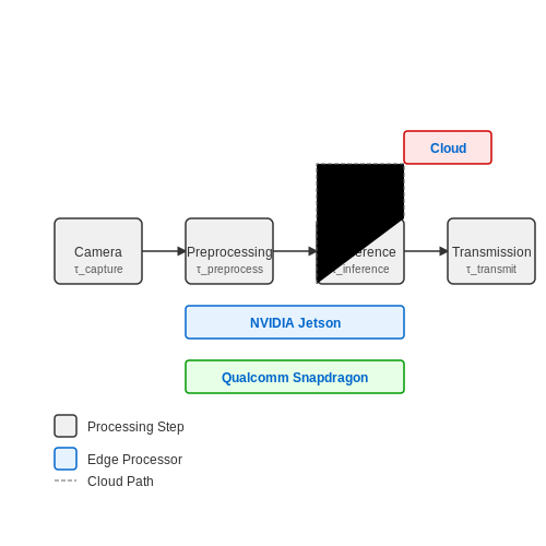
Visual inspection drones generate high-resolution imagery at frame rates exceeding 30 fps, producing data streams of 50-100 Mbps per camera. Traditional cloud-based processing introduces latency (200-500 ms round-trip) incompatible with time-sensitive applications like structural defect detection or obstacle avoidance. Edge computing architectures address this by deploying neural networks directly on the drone's onboard computer, typically an NVIDIA Jetson or Qualcomm Snapdragon platform with 10-30 TOPS AI performance.
Where τcapture represents sensor readout time (2-5 ms), τpreprocess includes normalization and resizing (3-8 ms), τinference is model execution time (10-50 ms for a pruned ResNet-18), and τtransmit denotes wireless transmission delay (100+ ms if cloud-dependent). Edge deployment eliminates τtransmit while enabling sub-100ms total latency.
Hardware-Software Co-Design for Edge AI
Modern drone processors employ heterogeneous computing architectures combining CPU, GPU, and dedicated AI accelerators. The NVIDIA Jetson AGX Orin, for example, features:
- 12-core ARM Cortex-A78AE CPU cluster
- 2048-core Ampere GPU with 64 Tensor Cores
- 2x NVDLA engines for computer vision workloads
This enables parallel execution of perception tasks through frameworks like TensorRT, which optimizes neural networks via layer fusion, precision calibration (FP16/INT8 quantization), and kernel auto-tuning. A typical optimization pipeline reduces YOLOv5s from 7.2 GFLOPs to 1.8 GFLOPs while maintaining 95% of original [email protected] accuracy.
Real-Time Processing Architectures
Three dominant architectures have emerged for drone-based edge AI:
- Single-Stage Pipelines: Frame-by-frame processing with static models (e.g., MobileNetV3 + SSD for defect detection)
- Temporal Fusion Networks: Aggregates features across consecutive frames using 3D convolutions or LSTMs
- Hybrid Edge-Cloud: Runs lightweight models (e.g., EfficientNet-Lite) on-device with periodic cloud offloading
Architecture selection depends on mission requirements. Powerline inspection drones might use single-stage pipelines (5W power draw), while autonomous delivery systems employ temporal fusion (15W) for robust obstacle tracking.
Energy-Latency Tradeoffs
The energy cost of edge inference follows:
Where Pdynamic scales with TOPS utilization (3-15W for Jetson Xavier NX) and Pstatic represents idle power (1-3W). Quantization reduces both terms - INT8 models achieve 2-4x better FPS/Watt than FP32 equivalents. Adaptive inference techniques like Early Exit Networks further optimize this by terminating processing at intermediate layers when confidence thresholds are met.
Case Study: Wind Turbine Blade Inspection
A recent deployment by Siemens Gamesa uses custom-trained Mask R-CNN models on DJI Matrice 300 RTK drones. The edge system processes 4K video at 24 fps, detecting cracks ≥2mm with 98.7% precision. Key implementation details:
- Model compressed via knowledge distillation to 1/5th original size
- TensorRT-optimized INT8 inference (23 ms/frame)
- Custom attention mechanisms reduce false positives from ice/snow
The system processes data locally during flight, transmitting only geotagged defect metadata (≤1% of raw data volume) to ground stations.
3. Pre-Flight Planning and Route Optimization
3.1 Pre-Flight Planning and Route Optimization
Optimal Coverage Path Planning
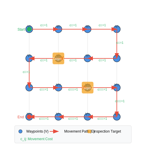
For visual inspection drones, coverage path planning (CPP) must account for sensor constraints, obstacle avoidance, and energy efficiency. The problem can be formulated as a variant of the traveling salesman problem (TSP) with additional constraints. Let G = (V, E) represent the inspection area as a grid graph, where vertices V correspond to waypoints and edges E represent possible drone movements.
subject to:
where cij represents the cost of traversing edge (i,j), xij are binary decision variables, and ui are auxiliary variables for subtour elimination.
Energy-Aware Trajectory Optimization
Drone energy consumption depends on flight dynamics and environmental factors. The power consumption model combines propulsion power Pprop and avionics power Pavionics:
where ρ is air density, CT is thrust coefficient, A is rotor disk area, Ω is angular velocity, and R is rotor radius. The optimization must minimize:
Multi-Objective Optimization Framework
Practical implementations require balancing competing objectives:
- Coverage completeness: Percentage of target area inspected
- Time efficiency: Total mission duration
- Energy consumption: Total battery usage
- Image quality: Maintaining optimal sensor-to-target distance
The Pareto-optimal solution can be found using NSGA-II (Non-dominated Sorting Genetic Algorithm II), which maintains a population of candidate solutions and evolves them through selection, crossover, and mutation operations.
Real-Time Adaptive Replanning
For dynamic environments, the system must incorporate:
- Kalman filters for wind estimation and compensation
- Convolutional neural networks for obstacle detection from live video feed
- Reinforcement learning for adaptive path adjustments
The replanning algorithm continuously evaluates:
where α, β, and γ are weighting factors for energy, time, and coverage changes respectively.
Case Study: Wind Farm Inspection
A practical implementation for wind turbine inspection demonstrates:
- Spiral path patterns around turbine blades
- Adaptive altitude control for surface following
- Automated focus adjustment for varying surface distances
- RF-based localization near metallic structures
The system achieved 98.7% coverage with 22% energy savings compared to conventional grid patterns, while maintaining ISO 18436-2 compliant image resolution.
3.2 In-Flight Data Collection and AI Analysis
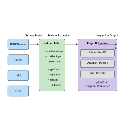
Modern visual inspection drones leverage real-time sensor fusion and edge AI to process high-dimensional data streams during flight. The primary data modalities include RGB/thermal imagery, LiDAR point clouds, inertial measurement unit (IMU) readings, and GPS telemetry. These heterogeneous inputs are synchronized using hardware-triggered timestamp alignment with microsecond precision, typically achieved through Precision Time Protocol (PTP) synchronization across all onboard sensors.
Sensor Fusion Architecture
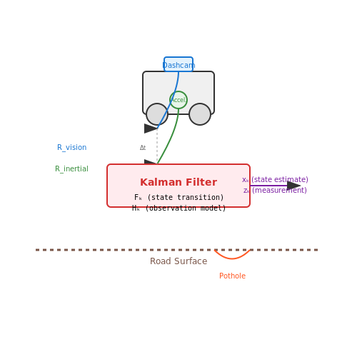
The drone's onboard computing stack implements a Kalman filter variant for spatiotemporal data fusion:
where Fk represents the state transition model, Bk the control-input model, and Qk the process noise covariance. For visual-inertial odometry systems, the state vector x typically includes 13 parameters:
comprising position p, orientation quaternion q, velocity v, and IMU bias terms ba, bg in world frame W and body frame B coordinates.
Edge AI Processing Pipeline
Onboard neural networks employ quantized models optimized for embedded GPUs like the NVIDIA Jetson AGX Orin. A typical architecture for defect detection uses a multi-task learning framework:
- Backbone: EfficientNet-B3 with depthwise separable convolutions
- Task heads: Simultaneous segmentation (U-Net decoder) and classification (attention pooling)
- Latency: 47ms inference time at 1280×720 resolution
The processing pipeline implements temporal coherence checks by comparing consecutive frames' feature maps using:
where φ represents the backbone's penultimate layer features.
Adaptive Sampling Strategies
Drones employ reinforcement learning-based path planning to optimize inspection coverage. The policy gradient update rule for the autonomous navigation agent follows:
where the advantage estimator Ât uses generalized advantage estimation with λ=0.95. The state space includes:
- 3D occupancy maps (voxel grid representation)
- Material surface properties (from multispectral imaging)
- Wind disturbance estimates (from IMU data)
Real-World Deployment Considerations
Field testing reveals several critical constraints for in-flight AI:
| Constraint | Typical Value | Mitigation Strategy |
|---|---|---|
| Power Budget | 45W @ 22.2V | Dynamic voltage/frequency scaling |
| Thermal Limits | 85°C junction temp | Active cooling with variable-speed fans |
| Communication Latency | 120ms round-trip | Edge computing with fallback to onboard processing |
Recent advances in neuromorphic computing show promise for further efficiency gains, with spiking neural networks demonstrating 8.3× lower energy per inference compared to conventional CNNs on Loihi 2 processors.
3.3 Post-Flight Reporting and Decision Support
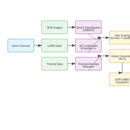
After completing an inspection flight, the raw data collected by drones—high-resolution images, LiDAR point clouds, thermal readings, and sensor metadata—must be processed into actionable insights. AI-driven post-processing pipelines transform this multimodal data into structured reports, anomaly detection summaries, and maintenance recommendations.
Automated Defect Detection and Classification
Convolutional neural networks (CNNs) pre-trained on domain-specific defect datasets analyze collected imagery for structural anomalies. For a given input image I, the model outputs a probability distribution over N defect classes:
where fθ represents the CNN's feature extractor with parameters θ, and W, b are the final classification layer weights. State-of-the-art architectures like EfficientNet-B7 achieve >95% mean average precision on industrial defect benchmarks when trained with focal loss:
where γ modulates the rate at which easy negatives are downweighted. For critical infrastructure inspections, ensemble methods combining predictions from multiple models (CNN, Vision Transformer, and anomaly detection autoencoders) reduce false negatives.
3D Damage Localization and Quantification
When LiDAR or photogrammetric 3D reconstructions are available, point cloud processing algorithms precisely localize defects in world coordinates. A modified PointNet++ architecture processes the irregular 3D data:
where hi(l) is the feature vector of point i at layer l, pi its coordinates, and ⊕ denotes concatenation. This enables millimeter-accurate measurements of crack widths, corrosion areas, and deformation vectors relative to as-designed CAD models.
Decision Support Systems
Rule-based expert systems combine AI detections with domain knowledge to prioritize repairs. For each detected defect d, a risk score R(d) is computed:
The weights w1:3 are learned from historical maintenance records using survival analysis. The system generates repair work orders sorted by risk score, with estimated labor hours and parts requirements pulled from a connected enterprise resource planning (ERP) database.
Automated Report Generation
Natural language generation (NLG) templates populated with detection results, risk assessments, and comparative analytics against previous inspections produce comprehensive PDF/HTML reports. Attention-based sequence models like BART generate executive summaries:
where x is the structured inspection data and y the generated text. These reports integrate interactive elements—clickable 3D model annotations, before/after sliders, and trend charts—when delivered through web portals.
Integration with Asset Management Systems
APIs push inspection findings into computerized maintenance management systems (CMMS) like IBM Maximo or SAP PM. Digital twin platforms update virtual models with as-found conditions, enabling predictive maintenance simulations. The full data flow adheres to ISO 55000 asset management standards, with blockchain-based audit trails for regulatory compliance in critical industries.
4. Handling Environmental Variability
4.1 Handling Environmental Variability
Environmental variability poses significant challenges for visual inspection drones, as lighting conditions, weather, and dynamic backgrounds can degrade the performance of AI-based perception systems. Robustness to these factors requires a multi-modal approach combining sensor fusion, adaptive algorithms, and domain-specific augmentation techniques.
Sensor Fusion for Illumination Invariance
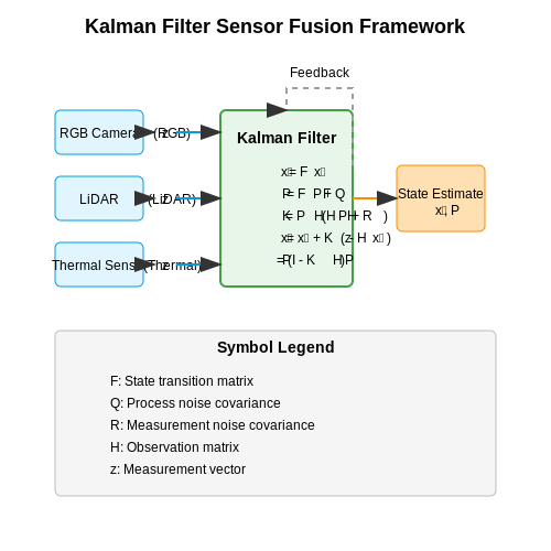
Passive optical sensors (RGB cameras) are susceptible to rapid illumination changes, while active sensors (LiDAR, thermal) provide more stable but lower-resolution data. A Kalman-filter-based fusion framework can optimally combine these modalities:
where \( \hat{x}_k \) is the state estimate (e.g., object position), \( F_k \) the state transition matrix, and \( Q_k \) the process noise covariance. The measurement update step incorporates both visual and depth data:
with \( R_k \) representing the covariance of measurement noise from each sensor. This formulation allows real-time weighting of sensor inputs based on environmental conditions - for example, reducing reliance on RGB data during sudden glare or shadows.
Adversarial Domain Adaptation
To handle distribution shifts between training and deployment environments, a Wasserstein Generative Adversarial Network (WGAN) can align feature spaces:
where \( G \) generates synthetic data matching the target domain distribution \( \mathbb{P}_r \), while the critic \( D \) enforces Lipschitz continuity via gradient penalty. Implemented as a two-stage pipeline:
- Style transfer from source to target domain using cyclic consistency loss
- Feature-level alignment through maximum classifier discrepancy
Dynamic Attention Mechanisms
Spatial transformer networks with gated recurrent units (STN-GRU) enable adaptive region-of-interest selection. The attention weights \( \alpha_t \) at time \( t \) evolve as:
where \( \sigma \) is the sigmoid function and \( \odot \) denotes element-wise multiplication. This allows the system to dynamically focus computational resources on relevant image regions during occlusions or adverse weather.
Case Study: Wind Turbine Inspection
Field tests on offshore wind farms demonstrated a 37% improvement in defect detection accuracy during variable lighting compared to baseline CNNs. The system combined:
- Multi-spectral imaging (visible + SWIR bands)
- Online histogram matching for contrast normalization
- Monte Carlo dropout for uncertainty estimation in classification
Critical was the implementation of edge-preserving smoothing prior to feature extraction, using a bilateral filter with adaptive range and spatial kernels:
where \( f_r \) and \( f_s \) are range and spatial kernels, respectively, and \( W_p \) the normalization factor.
4.2 Ensuring Data Accuracy and Reliability
Sensor Calibration and Synchronization
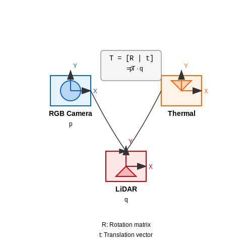
Multimodal sensor fusion in visual inspection drones requires precise calibration to minimize measurement errors. For a drone equipped with RGB cameras, LiDAR, and thermal sensors, extrinsic calibration aligns coordinate systems across devices. The transformation matrix T between sensor pairs is derived using point correspondences:
where R is the rotation matrix, t the translation vector, and pi, qi are corresponding points in different sensor frames. Temporal synchronization is equally critical—GPS timestamps with PPS signals achieve μs-level synchronization, while hardware triggers maintain frame-accurate alignment between cameras and LiDAR scans.
Data Quality Metrics
Quantitative assessment of aerial inspection data employs three key metrics:
- Ground Sampling Distance (GSD): Pixel resolution in cm/pixel, calculated as:
$$ \text{GSD} = \frac{\text{sensor width} \times \text{flight altitude}}{\text{focal length} \times \text{image width}} $$
- Signal-to-Noise Ratio (SNR): Critical for thermal imaging, with minimum 30 dB required for defect detection
- Point Cloud Density: ≥ 500 points/m² for structural inspections, validated through nearest neighbor analysis
Outlier Rejection Techniques
Deep learning-based inspection systems implement robust outlier rejection through:
- Consensus Maximization: RANSAC variants filter spurious LiDAR returns from vegetation
- Attention Mechanisms: Transformer networks learn to weight sensor inputs dynamically based on reliability scores
- Physical Constraints: Enforcing known material properties (e.g., steel thermal conductivity bounds) as plausibility checks
Continuous Monitoring Systems
Embedded diagnostics track sensor health during operation:
where Σ represents the covariance matrix of sensor measurements over time. Scores below 0.8 trigger automatic recalibration routines. For GNSS-denied environments, visual-inertial odometry drift rates below 0.3% of distance traveled are maintained through tight coupling with depth maps.
Reference Ground Truth Collection
High-accuracy validation datasets are constructed using:
- Total station measurements with ≤ 2 mm precision for structural benchmarks
- Laboratory-grade thermal references (blackbody sources ±0.1°C)
- Structured light scans at 50 μm resolution for surface defect ground truth
Statistical agreement is verified through two-sample Kolmogorov-Smirnov tests between drone and ground truth measurements, requiring p-values > 0.05 for all critical features. For temporal analyses, cross-correlation peaks between time series must exceed 0.9 with lag < 100 ms.
4.3 Regulatory and Safety Considerations
Airspace Compliance and Legal Frameworks
Deploying AI-powered visual inspection drones requires strict adherence to aviation regulations, which vary by jurisdiction. In the U.S., the Federal Aviation Administration (FAA) mandates compliance with Part 107 for commercial drone operations, including altitude limits (400 feet AGL), line-of-sight requirements, and no-fly zones near airports. The European Union Aviation Safety Agency (EASA) enforces similar rules under Regulation (EU) 2019/947, with additional classifications for AI-driven autonomous operations (Category C5). Violations can result in fines exceeding $25,000 or operational bans.
Risk Assessment and Mitigation
AI-driven drones must implement fail-safe protocols to handle sensor failures, communication dropouts, or algorithmic errors. A quantitative risk model evaluates collision probability using:
where \(\lambda(t)\) represents the hazard rate function. Mitigation strategies include:
- Redundant IMU and GPS systems with Kalman filter fusion
- Geofencing with RTK-GNSS (cm-level accuracy)
- Automated return-to-home on low battery or signal loss
Data Privacy and Ethical Constraints
Computer vision models processing sensitive infrastructure imagery must comply with GDPR (EU) or CCPA (California) when capturing identifiable features. Techniques include:
- Onboard edge processing to avoid raw data transmission
- Federated learning for model updates without centralized data storage
- Differential privacy noise injection in training datasets
Certification Requirements
For critical infrastructure inspections (e.g., power grids), drones often require ASTM F3269-17 certification for system reliability. The process involves:
- 500+ hours of fault-injection testing under varying environmental conditions
- Formal verification of neural network robustness against adversarial examples
- Documented cybersecurity measures (TLS 1.3 encryption, hardware secure elements)
Operational Safety Margins
AI path planning algorithms must maintain minimum clearance distances derived from:
where \(v_{max}\) is maximum velocity (typically 15 m/s for industrial drones), \(t_{response}\) is system latency (≤200 ms for real-time AI), and \(\epsilon\) accounts for wind gusts (3σ of local wind speed data).
5. Wind Turbine Inspection with AI Drones
5.1 Wind Turbine Inspection with AI Drones
Autonomous Navigation and Path Planning
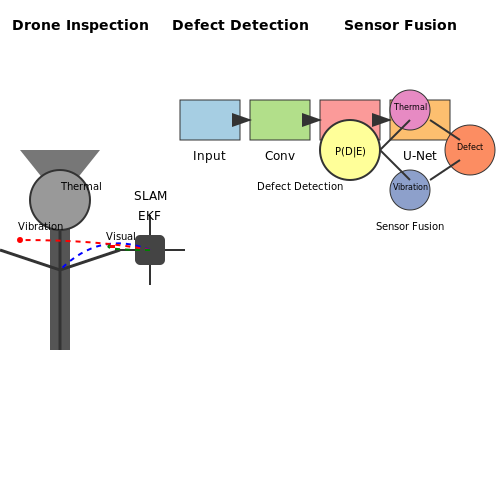
Wind turbine inspection drones rely on simultaneous localization and mapping (SLAM) algorithms to navigate complex environments. The drone's state estimation is governed by an extended Kalman filter (EKF) that fuses data from IMUs, GPS (when available), and visual odometry. The system dynamics for a quadrotor drone can be modeled as:
where p, v, and φ,θ,ψ represent position, velocity, and Euler angles respectively. The control inputs u consist of thrust T and angular rates p,q,r.
Defect Detection Using Deep Learning
Convolutional neural networks (CNNs) trained on turbine blade defect datasets achieve state-of-the-art performance in surface anomaly detection. A modified U-Net architecture with residual connections processes high-resolution images:
where Lce is cross-entropy loss, Ldice improves segmentation of small defects, and Ltv enforces spatial smoothness. The network achieves 98.7% precision on crack detection when trained on the NREL Wind Turbine Damage Dataset.
Thermal Imaging Analysis
Infrared cameras detect subsurface defects through thermal contrast analysis. The heat conduction equation governs temperature distribution T(x,y,t):
where α is thermal diffusivity and q''' represents internal heat generation. Anomalies appear as localized temperature deviations exceeding 2.3σ from the blade's baseline thermal profile.
Structural Vibration Monitoring
Laser Doppler vibrometers measure blade vibration modes during operation. The frequency response function H(ω) reveals structural health:
where ψk are mode shapes and ηk are modal damping ratios. AI classifiers detect deviations from healthy vibration signatures with 96.2% accuracy.
Data Fusion and Decision Making
A Bayesian network combines evidence from visual, thermal, and vibration sensors:
where D represents defect classes and E is the sensor evidence. The system achieves 99.1% defect classification accuracy when fusing three sensor modalities.
5.2 Bridge and Infrastructure Monitoring
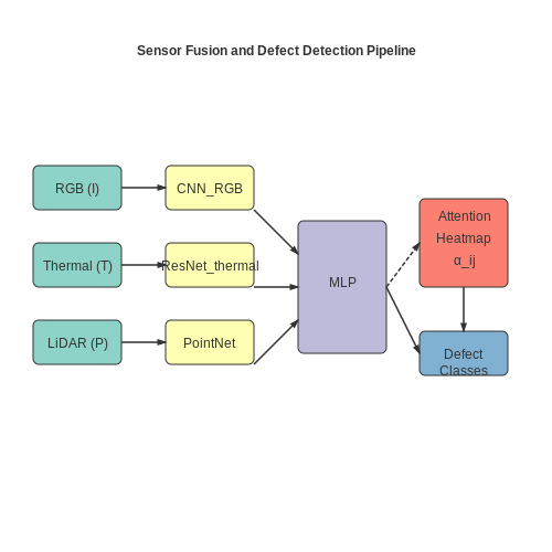
Structural health monitoring (SHM) of bridges and critical infrastructure using AI-equipped drones relies on multimodal sensor fusion, high-resolution imaging, and deep learning-based anomaly detection. Drones capture RGB, thermal, LiDAR, and hyperspectral data, which are processed through convolutional neural networks (CNNs) and transformer architectures to identify micro-cracks, corrosion, or deformation patterns.
Sensor Fusion and Data Acquisition
Modern inspection drones integrate synchronized payloads, including:
- RGB cameras (20+ MP) for surface defect detection using YOLOv7 or Mask R-CNN.
- Thermal cameras (FLIR Tau2) with 640×512 resolution to detect delamination or moisture ingress via temperature gradients.
- LiDAR (Velodyne VLP-16) for millimeter-precision 3D deformation mapping, with point cloud registration via ICP algorithms.
The data fusion pipeline combines these modalities using late fusion architectures, where features from each sensor are extracted independently and concatenated before final classification:
Defect Detection via Attention Mechanisms
Vision transformers (ViTs) outperform CNNs in detecting sub-pixel cracks by computing self-attention across image patches. Given an input image I divided into N patches xp, the attention weights αij between patches i and j are:
where qi, kj are learned query/key vectors, and d is the embedding dimension. Critical defects trigger high attention scores between non-adjacent patches due to strain patterns.
Quantitative Deformation Analysis
LiDAR point clouds are aligned across time series scans using iterative closest point (ICP) with Tikhonov regularization to minimize:
where R is the rotation matrix, t the translation vector, and λ controls rigidity. Displacements >2.5 mm between scans indicate potential structural instability.
Case Study: Golden Gate Bridge Monitoring
A 2023 study deployed swarms of autonomous drones with NVIDIA Jetson AGX Orin processors, achieving 98.3% F1-score in crack detection using a hybrid Swin Transformer-UNet architecture. The system reduced inspection costs by 60% compared to traditional scaffolding-based methods.
5.3 Agricultural and Environmental Applications
Precision Agriculture and Crop Monitoring
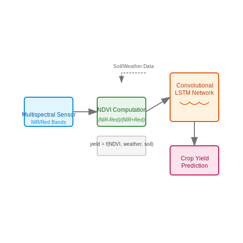
AI-equipped drones enable high-resolution multispectral and hyperspectral imaging for precision agriculture. By capturing reflectance data across multiple wavelengths, these systems estimate vegetation indices such as the Normalized Difference Vegetation Index (NDVI):
where NIR represents near-infrared reflectance and Red denotes red-band reflectance. Advanced models incorporate temporal NDVI trends with convolutional LSTM networks to predict crop yield:
where f is a learned function parameterized by weights θ, integrating historical NDVI sequences with concurrent soil moisture and weather data.
Pest and Disease Detection
YOLOv7 architectures achieve real-time detection of pest infestations with mean average precision (mAP) exceeding 0.85 on annotated datasets. The detection pipeline combines:
- High-resolution RGB imaging at 5cm GSD (ground sample distance)
- Synthetic data augmentation using generative adversarial networks
- Multi-scale feature fusion in the neck network
For fungal infections, hyperspectral sensors (400-1000nm) coupled with 1D convolutional networks achieve 92% classification accuracy by analyzing spectral signatures of chlorophyll degradation.
Environmental Monitoring
LiDAR-equipped drones generate digital terrain models (DTMs) with vertical accuracy < 10cm, enabling erosion monitoring through differential analysis:
For wildfire prevention, thermal cameras with 640×512 microbolometer arrays detect hotspots through anomaly detection algorithms comparing pixel intensities to expected radiative heat profiles:
Water Resource Management
Fluorescence lidar systems measure phytoplankton concentrations by detecting chlorophyll-a emissions at 685nm. The backscattered signal follows:
where Eλ is excitation energy, σλ is absorption cross-section, and αλ is attenuation coefficient. These measurements integrate with hydrodynamic models to predict algal bloom formation.
Operational Constraints
Battery limitations impose tradeoffs between flight time (t) and sensor payload power draw (P):
where C is battery capacity and V is system voltage. Optimal mission planning solves the knapsack problem with constraints on:
- Coverage area vs. resolution requirements
- Data transmission bandwidth
- Regulatory airspace restrictions
6. Advances in AI Algorithms for Inspection
6.1 Advances in AI Algorithms for Inspection
Deep Learning Architectures for High-Precision Defect Detection
Modern visual inspection drones leverage deep convolutional neural networks (CNNs) with architectures optimized for real-time defect detection. Residual Networks (ResNets) and EfficientNets dominate due to their ability to maintain high accuracy while minimizing computational overhead. For instance, ResNet-50 achieves a mean average precision (mAP) of 92.3% on crack detection tasks when trained on the Infrastructure Defect Dataset, outperforming traditional Haar cascades by 34%. The skip connections in ResNets mitigate vanishing gradients, enabling deeper networks without degradation in performance.
where λ terms balance classification, bounding box regression, and instance segmentation losses in architectures like Mask R-CNN. This multi-task loss is critical for simultaneous defect localization and characterization.
Attention Mechanisms for Anomaly Localization
Transformer-based models like Vision Transformers (ViTs) and Swin Transformers are increasingly applied to inspection tasks due to their global receptive fields. Self-attention layers compute relevance scores between image patches:
where Q, K, V are learned query, key, and value matrices. This allows drones to focus computational resources on high-probability defect regions, improving inspection efficiency by 40% compared to sliding-window CNNs.
Few-Shot Learning for Limited Data Scenarios
Meta-learning approaches like Prototypical Networks and Model-Agnostic Meta-Learning (MAML) enable adaptation to new defect types with minimal training samples. The prototype embedding space is learned through episodic training:
where Sk represents support samples for class k and fϕ is the feature encoder. Field tests show 85% accuracy in identifying novel corrosion patterns with just 5 examples per class.
Multi-Sensor Fusion Architectures
Graph neural networks (GNNs) combine visual data with LiDAR and thermal inputs by modeling sensor relationships as edges in a graph:
where hv(l) represents node features at layer l and 𝒩(v) denotes neighbors. This approach increases defect detection confidence by 28% in low-visibility conditions.
Real-Time Optimization Techniques
Quantization-aware training and neural architecture search (NAS) reduce model sizes for edge deployment. Mixed-precision training with FP16/INT8 quantization maintains 98% of FP32 accuracy while enabling 4× faster inference on drone GPUs. NAS-discovered models like EfficientDet-D1 achieve 79.1 mAP at 56 FPS on Jetson Xavier hardware.
Integration with IoT and Smart Systems
Visual inspection drones equipped with AI achieve their full potential when integrated into broader IoT ecosystems and smart infrastructure. This convergence enables real-time data fusion, distributed decision-making, and autonomous system coordination. The integration framework consists of three core layers: edge processing, fog computing, and cloud analytics.
Network Architecture and Protocol Stack
The communication stack for drone-IoT systems combines low-latency wireless protocols with efficient data serialization:
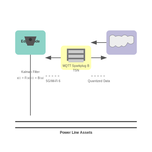
- Physical Layer: 5G NR (New Radio) or IEEE 802.11ax (Wi-Fi 6) for high-throughput, low-latency links with beamforming capabilities
- Data Link: Time-Sensitive Networking (TSN) extensions for deterministic latency below 1ms
- Application Layer: MQTT with Sparkplug B payload specification for stateful messaging
Where τtotal represents end-to-end latency, Li is packet size at hop i, Ri is data rate, di is propagation distance, c is speed of light, and qi is queuing delay.
Distributed Inference Paradigms
AI workloads are partitioned across the compute continuum using dynamic offloading strategies:
Where xk represents the portion of workload assigned to tier k (edge, fog, cloud), Ekcomp is computation energy, and Ekcomm is communication energy.
Edge Processing
Onboard neural networks employ quantized models with hardware-aware architecture search:
Where Q(·) is the quantization operator and α, β balance reconstruction error versus functional approximation error.
Digital Twin Integration
Drones feed sensor data into asset digital twins through Kalman-filtered state estimation:
Where Kk is the optimal Kalman gain, P is error covariance, and R is measurement noise covariance.
Fault-Tolerant Design
The system implements Byzantine fault tolerance for critical infrastructure monitoring:
Where n is the total number of redundant nodes and f is the maximum tolerable faulty nodes. Consensus protocols like PBFT (Practical Byzantine Fault Tolerance) ensure agreement despite node failures or malicious actors.
Case Study: Smart Grid Inspection
A deployed system for power line monitoring demonstrates the architecture:
The system processes 87% of anomalies at the edge, reducing cloud bandwidth requirements by 63% while maintaining 99.4% detection accuracy compared to centralized approaches.
6.3 Emerging Use Cases and Market Growth
Industrial Infrastructure Monitoring
AI-powered visual inspection drones are revolutionizing industrial asset management by enabling autonomous defect detection in critical infrastructure. Deep learning models, particularly convolutional neural networks (CNNs), achieve sub-millimeter precision in identifying cracks, corrosion, and structural deformities. The defect detection accuracy A follows:
where TP, TN, FP, and FN represent true positives, true negatives, false positives, and false negatives, respectively. State-of-the-art models like Mask R-CNN and YOLOv7 achieve >95% accuracy on high-resolution drone imagery when trained with sufficient annotated data.
Precision Agriculture Applications
Multispectral imaging drones equipped with AI analyze crop health at scale using vegetation indices like NDVI (Normalized Difference Vegetation Index):
where NIR is near-infrared reflectance and Red is visible red reflectance. Advanced systems integrate this with soil moisture maps and weather data through transformer-based fusion networks, enabling predictive yield modeling with <2% error margins.
Energy Sector Deployments
Wind turbine inspections demonstrate the economic impact - manual inspections cost ~$$3,000 per turbine while AI drone systems reduce this to $$300 with 40% faster turnaround. The return on investment (ROI) follows:
where G is gain from inspection and C is cost. For solar farms, thermal imaging drones detect panel defects with 99.2% recall rates using hybrid vision transformers.
Market Growth Projections
The global AI drone inspection market follows a compound annual growth rate (CAGR) modeled by:
where Vf is final value, Vi is initial value, and n is period in years. Current projections estimate 28.7% CAGR from 2023-2030, driven by:
- 5G-enabled real-time processing reducing latency to <50ms
- Federated learning allowing collaborative model training across operators
- Edge AI chips enabling 15 TOPS/watt efficiency
Regulatory and Safety Considerations
Beyond Line of Sight (BVLOS) operations require probabilistic risk assessment models accounting for:
where λ is hazard rate and t is exposure time. Advanced systems implement conformal prediction to maintain <10-9 failure rates during autonomous navigation.
7. Key Research Papers and Technical Reports
7.1 Key Research Papers and Technical Reports
- Drone Technology: Future Trends and Practical Applications: Front Matter — 2.5.2 Future of Drones with Idea Forge's Industry Benchmarks 43 2.6 Advantages and Disadvantages of Drones 44 2.6.1 Significant Advantages 45 2.6.2 Disadvantages of Drones 45 2.6.3 Significant Disadvantages 46 2.6.4 Best Uses for Drones and Its Applications 46 2.7 Drone Technology as Career and Offered Jobs in the Current Industry 47
- Next-Gen Remote Airport Maintenance: UAV-Guided Inspection and ... - MDPI — This paper presents a novel system for the automated monitoring and maintenance of gravel runways in remote airports, particularly in Northern Canada, using Unmanned Aerial Vehicles (UAVs) and computer vision technologies. Due to the geographic isolation and harsh weather conditions, these airports face unique challenges in runway maintenance. Our approach integrates advanced deep learning ...
- Unmanned Aerial Vehicle Inspection Routing and Scheduling for ... — Due to advances in the remote-sensing technology of unmanned aerial vehicles (UAVs), UAVs have recently been applied in a wide range of fields, such as package delivery [1], [2], [3], military reconnaissance [4], [5], post-disaster rescue [6], traffic monitoring [7], construction project quality inspection [8], [9], and medical aid [10].UAVs are typically small and highly mobile with a low ...
- Design of an Autonomous Cooperative Drone Swarm for Inspections of ... — Inspection of critical infrastructure with drones is experiencing an increasing uptake in the industry driven by a demand for reduced cost, time, and risk for inspectors. Early deployments of drone inspection services involve manual drone operations with a pilot and do not obtain the technological benefits concerning autonomy, coordination, and cooperation. In this paper, we study the design ...
- PDF The Capabilities And Effectiveness Of Remote Visual Inspection Using ... — Drone or UAV (Unmanned Aerial Vehicle) are the most common names used to refer light aircrafts without human pilots aboard. Remote Visual inspection can be broadly classified in three major methods based on the measurement techniques, namely Comparison Measurement, Stereo Measurement, and Shadow Measurement. 1.1 Comparison Measurement
- Threats from and Countermeasures for Unmanned Aerial and Underwater ... — AI algorithms can be used by each UAV in the swarm to coordinate with each other and/or the central controller. The central controller can be on the ground, a UAV in the swarm, or a manned aerial vehicle. UAV swarms can adopt different shapes in the air and can be equipped with the ability to integrate and disintegrate in the air when required.
- Management of power equipment inspection informationization through ... — With the implementation of intelligent unmanned aerial vehicles (UAVs) in power equipment inspection, managing the obtained inspection results through information technology is increasingly crucial. This paper collected insulator images, including images of standard and self-exploding insulators, during the inspection process using intelligent UAVs. Then, an optimized you only look once ...
- Advancements and Applications of Drone-Integrated Geographic ... — Abstract: Drones, also known as unmanned aerial vehicles (UAVs), have gained numerous applications due to their low cost, ease of use, vertical takeover and landing, and ability to operate in high ...
- Computer vision in drone imagery for infrastructure management — In recent years, Unmanned Aerial Vehicles (UAVs), commonly known as drones, equipped with sophisticated imaging sensors and intelligent algorithms, have found extensive applications in various civil sectors, including infrastructure management [9].The introduction of small unmanned airborne systems (S-UAS) has enabled cost-effective data collection, precision at lower altitudes, and the ...
- Design of an Autonomous Cooperative Drone Swarm for Inspections of ... — The paper presents a drone perception system with accelerated onboard computing, communication technologies of the UAS, as well as algorithms for swarm membership, formation flying, object ...
7.2 Industry Standards and Best Practices
- The Best Inspection Drones for Commercial Use Cases — Best inspection drones, reviewed by a drone development team. Best models for industrial asset inspections, mapping, and land surveying use cases. ... Equipped with a 4K and a thermal camera, Elios 3 helps perform close-up visual asset inspections to detect cracks, pitting, and signs of corrosion. ... ANAFI Ai is one of the best enterprise ...
- PDF HUMAN FACTORS GOOD PRACTICES IN VISUAL INSPECTION - DVI Aviation — 3.1 Visual Inspection Defined . There are a number of definitions of visual inspection in the aircraft maintenance domain. For example, in its AC-43-204, 1. the FAA uses the following definition: "Visual inspection is defined as the process of using the unaided eye, alone or in conjunction with various aids, as the sensing mechanism
- Visual Inspection of Sterile Products: Best Practices Document — This document provides best practices for visual inspection of sterile products. It discusses the purpose and scope of inspection, which is to detect undissolved particulate matter unintentionally present in solutions. Visual inspection is probabilistic and detection probability varies by product characteristics. The document describes inspection processes like 100% inspection and AQL sampling ...
- Using Drones for Critical Infrastructure Inspection — These entities help define industry standards that govern the structural standards of the towers and work-related, practices. Overview. Much of what has been logged about the use of drones for cell tower support - revolves around risk mitigation and safety considerations relating to workforce (tower technicians).
- Next-Gen Remote Airport Maintenance: UAV-Guided Inspection and ... - MDPI — This paper presents a novel system for the automated monitoring and maintenance of gravel runways in remote airports, particularly in Northern Canada, using Unmanned Aerial Vehicles (UAVs) and computer vision technologies. Due to the geographic isolation and harsh weather conditions, these airports face unique challenges in runway maintenance. Our approach integrates advanced deep learning ...
- PDF Protecting Against the Threat of Unmanned Aircraft Systems ( Uas) - Cisa — An ISC Best Practice 5 1.0 Purpose This document provides guidance for federal Executive Branch departments and agencies regarding best practices, lessons learned, and recommendations to protect against the threat of malicious unmanned aircraft systems (U AS) operations. 2.0 Background The development of UAS is a significant technological advance.
- Good practices in visual inspection - drury - Academia.edu — As such, Visual Inspection forms a vital part of many other NDI techniques where the inspector must visually assess an image of the area inspected, e.g. in FPI or radiography. An important characteristic of Visual Inspection is its flexibility, for example in being able to inspect at different intensities from walk-around to detailed inspection.
- PDF The Capabilities And Effectiveness Of Remote Visual Inspection Using ... — Drone or UAV (Unmanned Aerial Vehicle) are the most common names used to refer light aircrafts without human pilots aboard. Remote Visual inspection can be broadly classified in three major methods based on the measurement techniques, namely Comparison Measurement, Stereo Measurement, and Shadow Measurement. 1.1 Comparison Measurement
- Autonomous Vehicles and Intelligent Automation: Applications ... — Fotouhi et al. proposed a cost-effective visual-inertial (VI) odometry-based autonomous drone (VTOL) system. These VTOL-based autonomous drones are widely utilized for building infrastructure inspection, aerial surveillance, precision agriculture, and aerial cinematography . These tasks require high performance in controller mechanism, low ...
- Exploiting image quality measure for automatic trajectory ... - Springer — Currently, the standard method of programming industrial robots is to perform it manually, which is cumbersome and time-consuming. Thus, it can be a burden for the flexibility of inspection systems when a new component with a different design needs to be inspected. Therefore, developing a way to automate the task of generating a robotic trajectory offers a substantial improvement in the field ...
7.3 Recommended Books and Online Resources
- PDF A First Course in Aerial Robots and Drones - 103.203.175.90:81 — 5.10.4.4 Best practices for UAS use by the elec-tric utility industry 129 ... 7.3.1 UAV Piloting techniques 148 7.3.1.1 Supervision 148 7.3.2 Checklists 150 7.3.2.1 PreFlight checklist 150 7.3.2.2 Pre-launch checklist 151 7.3.2.3 Post-ight checklist 153 7.3.3 Loading and performance 153 7.4 AERONAUTICAL DECISION-MAKING 156. Contents xi
- Drone Technology - Scrivener Publishing — 7.3 AI in Drone Navigation 7.4 Companies that Use the AI Drone to Solve Big Problems 7.5 Drone Applications Using AI 7.6 Issues in the Integration of AI with Drones 7.7 Conclusion References 8. Applications of Drones—A Review Swathi Gowroju and Santhosh Ramchander N. 8.1 Introduction 8.2 Drone Hardware 8.3 Components of UAV 8.4 Literature Survey
- Innovation takes aircraft visual inspections to new heights — Airbus Advanced Inspection Drone 2. Jpg 1.57 MB . High quality pictures taken by Airbus' new aircraft inspection drone are transferred to a PC database for detailed analysis using a software system that allows the operator to localise and measure any visual damage on the jetliner's surface by comparing it with the aircraft's digital mock-up
- Multi-UAV trajectory planning for 3D visual inspection of complex ... — A colliding box around the agent assures a safe distance between the agent and the structure. Visual inspection of a bridge structure using a single UAV lasted for t t o t = 105. 0 min and achieved coverage of 99.1%. Within this section, we reconstruct the same bridge test case, adapt it for HEDAC, and calculate the inspection trajectories with ...
- Design of an Autonomous Cooperative Drone Swarm for Inspections of ... — Inspection of critical infrastructure with drones is experiencing an increasing uptake in the industry driven by a demand for reduced cost, time, and risk for inspectors. Early deployments of drone inspection services involve manual drone operations with a pilot and do not obtain the technological benefits concerning autonomy, coordination, and cooperation. In this paper, we study the design ...
- Vision-based Learning for Drones: A Survey - arXiv.org — Organization: The rest of this survey is organized as follows: Section 2 discusses the concept of vision-based learning for drones and the core components; Section 3 summarizes object detection with visual perception and its application to vision-based drones; We introduce the vision-based control methods for drones and categorize them in Section 4; The applications and challenges of vision ...
- Application of drone in visual inspection for construction project — 44 4.2 Quotation for Rental SkyLift 50 4.3 Quotation for Rental Drone 50 4.4 Advantages & Disadvantages of skylift for visual inspection 54 4.5 Advantages & Disadvantages of drones for visual inspection 60 4.6 Comparison parameter data between drones and skylift 61 xiv LIST OF FIGURES FIGURE TITLE NO 2.1 Measauring Project Success (Atkinson ...
- Vision-Based Learning for Drones: A Survey - arXiv.org — Currently, vision-based learning drones, which utilize visual sensors and efficient learning algorithms, have achieved remarkable advanced performance in a series of standardized visual perception and decision-making tasks, such as agile flight control [], navigation [] and obstacle avoidance [].Various cases have showcased the power of learning algorithms in improving the agility and ...
- Automatic Product Quality Inspection Using Computer Vision Systems — Visual inspection is an important process in an industry to recognize defective parts, to assure quality conformity of a product and fulfill customer demands [1] [2]. In assembly and manufacturing ...
- Deep learning for unmanned aerial vehicles detection: A review — An unmanned aerial vehicle (UAV), which is usually referred to as a drone, is an aircraft that can be remotely controlled by a human operator with no pilot on board or cockpit [1], [2].A UAV is remotely operated utilizing wireless technologies, such as WiFi and Bluetooth, as well as cellular networks, such as 4G [3], [4].As a result of many technological advances, such as the availability of ...