Voice Command Recognition for Smart Homes
1. Acoustic Signal Processing Basics
1.1 Acoustic Signal Processing Basics
Time-Domain Representation of Sound
Acoustic signals are fundamentally pressure waves propagating through a medium, typically air. In the time domain, a sound wave x(t) is represented as a continuous function of pressure variation over time. For discrete-time processing, such as in digital voice recognition systems, the signal is sampled at a rate fs satisfying the Nyquist criterion:
where fmax is the highest frequency component of interest. For speech signals, a sampling rate of 16 kHz is common, capturing frequencies up to 8 kHz.
Frequency-Domain Analysis
Time-domain signals are transformed into the frequency domain using the Discrete Fourier Transform (DFT):
where x[n] is the discrete-time signal, N is the frame length, and X[k] represents the complex spectral components. The Short-Time Fourier Transform (STFT) applies the DFT to overlapping windowed segments of the signal, providing a time-frequency representation:
Here, w[n] is a window function (e.g., Hamming), m is the frame index, and H is the hop size.
Mel-Frequency Cepstral Coefficients (MFCCs)
MFCCs are a compact representation of the spectral envelope, optimized for speech recognition. The computation involves:
- Power Spectrum: Compute the squared magnitude of the STFT.
- Mel Filterbank: Apply triangular filters spaced according to the Mel scale, which approximates human auditory perception:
- Log Compression: Take the logarithm of the filterbank energies to de-emphasize high-energy components.
- Discrete Cosine Transform (DCT): Decorrelate the filterbank energies to yield cepstral coefficients.
Pre-Emphasis and Windowing
Pre-emphasis compensates for the natural 6 dB/octave roll-off in speech spectra:
where α ≈ 0.97. Windowing (e.g., Hamming) minimizes spectral leakage in the STFT:
Real-World Considerations
In smart home environments, acoustic signals are often corrupted by background noise (e.g., appliances, echoes). Spectral subtraction or Wiener filtering can mitigate this. For far-field voice recognition, beamforming techniques using microphone arrays enhance signal-to-noise ratio by spatially filtering sound sources.

Feature Extraction Techniques (MFCC, Spectrograms)
Feature extraction is a critical step in voice command recognition, transforming raw audio signals into compact, discriminative representations suitable for machine learning models. Two dominant techniques in speech processing are Mel-Frequency Cepstral Coefficients (MFCCs) and spectrograms, each capturing distinct aspects of the audio signal.
Mel-Frequency Cepstral Coefficients (MFCCs)
MFCCs are engineered to approximate the human auditory system's response, making them highly effective for speech recognition. The extraction pipeline involves the following steps:
- Pre-emphasis: High-frequency components are amplified to balance the signal's energy spectrum. The pre-emphasized signal y[n] is computed as:
$$ y[n] = x[n] - \alpha x[n-1] $$where α typically ranges between 0.95 and 0.97.
- Framing and Windowing: The signal is divided into short, overlapping frames (20–40 ms) to assume quasi-stationarity. A Hamming window is applied to minimize spectral leakage:
$$ w[n] = 0.54 - 0.46 \cos\left(\frac{2\pi n}{N-1}\right) $$where N is the frame length.
- Discrete Fourier Transform (DFT): Each windowed frame is converted to the frequency domain via DFT, yielding the power spectrum:
$$ P[k] = \left|\sum_{n=0}^{N-1} y[n] w[n] e^{-j 2\pi kn/N}\right|^2 $$
- Mel Filterbank Application: The power spectrum is mapped to the Mel scale, which linearizes frequency perception below 1 kHz and logarithmizes it above. A triangular filterbank with 20–40 filters is applied:
$$ \text{Mel}(f) = 2595 \log_{10}\left(1 + \frac{f}{700}\right) $$
- Logarithm and DCT: The log of filterbank energies is computed, followed by a Discrete Cosine Transform (DCT) to decorrelate coefficients. The first 12–20 coefficients are retained as MFCCs.
Spectrograms
Spectrograms provide a time-frequency representation of the audio signal, visualizing how spectral components evolve over time. The process involves:
- Short-Time Fourier Transform (STFT): The signal is segmented into frames, and DFT is applied to each. The magnitude spectrum of each frame is stacked to form a 2D matrix:
$$ S[t, k] = \left|\sum_{n=0}^{N-1} x[n] w[n - tH] e^{-j 2\pi kn/N}\right| $$where H is the hop size between frames.
- Log Scaling: The magnitude spectrogram is often log-scaled (dB) to enhance perceptual relevance:
$$ S_{\text{log}}[t, k] = 10 \log_{10}(S[t, k] + \epsilon) $$where ε is a small constant to avoid numerical instability.
Practical Considerations
- MFCCs vs. Spectrograms: MFCCs are computationally efficient and robust to noise but discard phase information. Spectrograms retain full time-frequency data but require deeper models (e.g., CNNs) for processing.
- Hyperparameter Tuning: Frame length, hop size, and Mel filter count must balance temporal resolution (shorter frames) and frequency resolution (longer frames). Typical values are 25 ms frames with a 10 ms hop.
- Real-time Processing: For smart home applications, MFCCs are preferred due to their lower dimensionality, enabling faster inference on edge devices.

1.3 Speech-to-Text Conversion Models
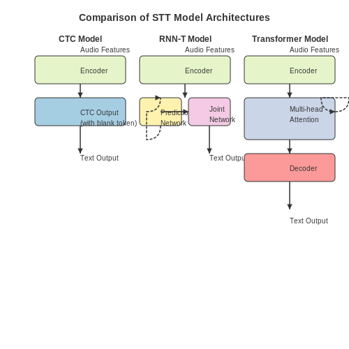
Modern speech-to-text (STT) systems leverage deep learning architectures to achieve high accuracy in transcribing spoken language into written text. The dominant approaches include connectionist temporal classification (CTC), recurrent neural network transducers (RNN-T), and transformer-based models, each with distinct advantages in handling temporal alignment and contextual dependencies.
Connectionist Temporal Classification (CTC)
CTC addresses the challenge of aligning variable-length audio sequences with corresponding text transcripts by introducing a blank token and allowing repetitions. Given an input sequence x of length T, the model outputs a probability distribution over the vocabulary (including blank) at each timestep. The CTC loss function marginalizes over all possible alignments:
where π represents a path, y is the target sequence, and ℬ is the function that collapses repeated characters and removes blanks. Practical implementations often use beam search with language model integration during inference to improve fluency.
Recurrent Neural Network Transducers (RNN-T)
RNN-T extends CTC by incorporating a prediction network that models dependencies in the output sequence. The architecture consists of:
- An encoder network processing acoustic features
- A prediction network modeling label history
- A joint network combining both representations
The joint output distribution at each timestep (t,u) is computed as:
where ht and gu are the encoder and prediction network outputs respectively. RNN-T achieves superior performance on conversational speech by explicitly modeling output dependencies, though at increased computational cost.
Transformer-Based Models
Recent architectures like Whisper and Conformer replace recurrent layers with self-attention mechanisms. The multi-head attention computes:
where Q, K, and V are learned linear projections of the input. Transformer models excel at capturing long-range dependencies through stacked attention layers, with convolutional modules (in Conformers) improving local feature extraction. State-of-the-art systems often employ:
- SpecAugment for robust acoustic modeling
- Byte-pair encoding for subword tokenization
- Teacher-student distillation for efficiency
Practical Deployment Considerations
For smart home applications, model optimization techniques become critical:
where nchunks depends on the streaming window size. Quantization-aware training reduces model size by representing weights as 8-bit integers (INT8) with minimal accuracy loss:
Edge deployment typically uses TensorFlow Lite or ONNX Runtime with hardware-specific acceleration through DSPs or NPUs.
2. Supervised Learning Approaches (HMMs, CNNs, RNNs)
2.1 Supervised Learning Approaches (HMMs, CNNs, RNNs)
Hidden Markov Models (HMMs) for Speech Recognition
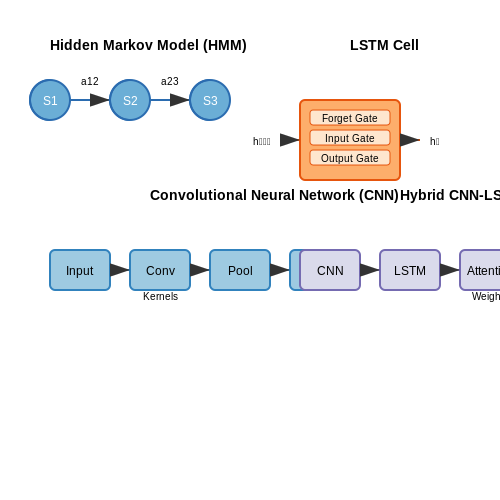
Hidden Markov Models have been a cornerstone of speech recognition systems since the 1980s. An HMM represents speech as a sequence of states, where each state emits observable acoustic features while transitions between states follow probabilistic rules. For a speech signal x1:T and a sequence of words W, the recognition task reduces to finding:
The Viterbi algorithm efficiently computes this by dynamic programming, with time complexity O(TN2) for N states. Modern implementations use Gaussian Mixture Models (GMMs) for emission probabilities:
Convolutional Neural Networks (CNNs) for Spectrogram Analysis
CNNs process speech through hierarchical feature extraction from spectrograms. A typical architecture for voice commands includes:
- 2-3 convolutional layers with ReLU activation and max pooling
- Kernel sizes of 5×5 to 9×9 in time-frequency domain
- Batch normalization between layers
- Global average pooling before dense classification layers
The convolution operation for a spectrogram input X with kernel K at position (i,j) is:
Recurrent Neural Networks (RNNs) for Temporal Modeling
Long Short-Term Memory (LSTM) networks address vanishing gradients in standard RNNs through gating mechanisms. The LSTM cell updates at time t follow:
Bidirectional LSTMs process sequences in both directions, capturing contextual information from past and future frames simultaneously.
Hybrid Architectures
State-of-the-art systems combine these approaches:
- CNN-LSTM: CNNs extract local features fed to LSTMs for temporal modeling
- Attention Mechanisms: Weighted frame importance improves recognition of key phonemes
- End-to-End Models: Connectionist Temporal Classification (CTC) loss enables direct speech-to-text mapping
The CTC objective for target sequence y and input x is:
where ℬ is a function that collapses repeated labels and removes blank tokens.
Practical Implementation Considerations
For smart home applications with limited compute resources:
- Quantization reduces model size (e.g., FP32 → INT8) with minimal accuracy loss
- Pruning removes redundant weights below a threshold
- Knowledge distillation trains compact student models from larger teacher models
The distillation loss combines task loss Ltask and distillation loss Ldistill:
where T is the temperature parameter controlling soft target smoothness.
End-to-End Deep Learning Models (Transformers, Wav2Vec)
Transformer Architectures for Speech Recognition
Traditional automatic speech recognition (ASR) systems relied on hybrid architectures combining convolutional neural networks (CNNs), recurrent neural networks (RNNs), and hidden Markov models (HMMs). Transformers have emerged as a superior alternative due to their ability to model long-range dependencies in sequential data through self-attention mechanisms. The key innovation lies in the attention weights that dynamically focus on relevant parts of the input sequence:
where Q, K, and V represent queries, keys, and values matrices respectively, and dk is the dimension of the key vectors. For speech processing, the input consists of mel-spectrogram frames or raw waveform chunks, which the transformer processes in parallel rather than sequentially.
Wav2Vec 2.0 Architecture
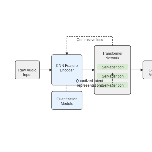
Wav2Vec 2.0 introduces a self-supervised learning framework that learns speech representations from raw audio. The model consists of:
- A multi-layer CNN feature encoder that processes raw waveforms into latent representations
- A transformer network that builds contextualized representations
- A quantization module that discretizes the continuous speech representations
The model is pretrained using a contrastive loss where the system must identify the true quantized latent speech representation among distractors:
where ct is the context vector, qt is the true quantized vector, and Qt contains both the true quantized vector and distractors.
Fine-tuning for Voice Command Recognition
For smart home applications, pretrained models are fine-tuned on domain-specific command datasets. The process involves:
- Adding a classification head on top of the transformer
- Training with connectionist temporal classification (CTC) loss for sequence alignment
- Optimizing for low-latency inference on edge devices
The CTC loss function handles the alignment between variable-length audio inputs and output sequences:
where π represents a path through the output tokens, x is the input sequence, and yπtt is the probability of token πt at time t.
Practical Implementation Considerations
Deploying these models in smart home environments requires addressing several challenges:
- Model compression: Knowledge distillation and quantization to reduce model size
- Wake word detection: Implementing efficient always-on detection
- Adaptation: Continual learning to handle new commands and accents
Recent advancements like conformer architectures combine the strengths of transformers and CNNs, achieving state-of-the-art results with fewer parameters. These hybrid models use depthwise separable convolutions in the feed-forward layers:
where Cin equals the input channel dimension, significantly reducing computational complexity while maintaining performance.
2.3 Handling Ambiguity and Noise in Voice Commands
Signal-to-Noise Ratio Optimization
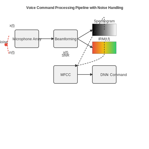
Voice command recognition in smart homes must contend with environmental noise, microphone quality, and speech variability. The signal-to-noise ratio (SNR) is a critical metric for evaluating system robustness. For a given input signal x(t) corrupted by additive noise n(t), the SNR is defined as:
where Psignal and Pnoise represent the power of the clean speech and noise components, respectively. Practical systems require SNR values above 15 dB for reliable recognition. Beamforming techniques using microphone arrays can improve SNR by spatially filtering noise:
where wi are adaptive weights and τi are time delays compensating for wavefront arrival differences.
Feature Space Robustness
Mel-frequency cepstral coefficients (MFCCs) remain the dominant feature representation, but their sensitivity to noise necessitates augmentation. Delta and delta-delta coefficients capture temporal dynamics, while cepstral mean and variance normalization (CMVN) reduces channel effects:
where μc and σc are the mean and standard deviation of cepstral coefficients. Recent approaches incorporate time-frequency masking in the spectrogram domain before MFCC computation, using neural networks to predict ideal ratio masks (IRMs):
Acoustic Model Adaptation
Deep neural network (DNN) acoustic models benefit from multi-condition training with additive noise and room impulse responses. Data augmentation strategies include:
- Adding noise samples from the DEMAND database at varying SNRs
- Applying random bandpass filtering (300-4000 Hz) to simulate telephone channels
- Convolving with measured room impulse responses
For domain adaptation, teacher-student learning with noisy inputs to the student model and clean references from the teacher has shown particular promise. The Kullback-Leibler divergence loss enforces distribution matching:
Language Model Rescoring
N-best list rescoring with contextual language models mitigates lexical ambiguity. Transformer-based models capture long-range dependencies better than traditional n-grams. Given acoustic model scores PAM(W|X) and language model scores PLM(W), the final hypothesis is selected via:
where λ is tuned on a development set. For smart home applications, domain-specific language models trained on home automation corpora yield 15-20% relative error reduction compared to general-purpose models.
Endpoint Detection
Robust voice activity detection (VAD) prevents false triggers from non-speech sounds. Energy-based thresholds fail under noise, making neural VAD essential. A typical architecture uses a BiLSTM processing 40ms frames:
where ptspeech is the speech probability at frame t. Decision smoothing with hidden Markov models (HMMs) avoids rapid state transitions.
3. IoT Communication Protocols (MQTT, Zigbee)
IoT Communication Protocols (MQTT, Zigbee)
MQTT (Message Queuing Telemetry Transport)
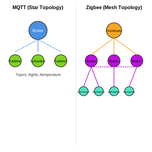
MQTT operates on a publish-subscribe architecture, where clients communicate through a central broker rather than directly with each other. The protocol uses TCP/IP for reliable message delivery and supports three Quality of Service (QoS) levels:
- QoS 0 (At most once): Messages are delivered with no acknowledgment or retransmission.
- QoS 1 (At least once): Messages are guaranteed to arrive but may be duplicated.
- QoS 2 (Exactly once): Messages are guaranteed to arrive exactly once through a four-step handshake.
The protocol efficiency stems from its minimal header size (2 bytes minimum) and binary payload format. The publish-subscribe pattern scales well for IoT deployments where thousands of devices may connect to a single broker. The retained messages feature allows new subscribers to immediately receive the last known good state of a topic.
For smart home applications, MQTT's lightweight nature makes it ideal for battery-powered sensors transmitting intermittent updates. The protocol supports TLS encryption for secure communication, though the computational overhead may be prohibitive for some constrained devices.
Zigbee Protocol Stack
Zigbee builds upon the IEEE 802.15.4 standard for low-rate wireless personal area networks, adding network and application layers to create a full protocol stack. The physical layer operates in three frequency bands:
- 868 MHz (Europe) with a data rate of 20 kbps
- 915 MHz (Americas) with 40 kbps
- 2.4 GHz (worldwide) with 250 kbps
The network layer handles device addressing using 16-bit short addresses alongside 64-bit IEEE addresses. Zigbee supports three device types:
- Coordinator: Forms the network and maintains routing tables
- Router: Extends network coverage and relays messages
- End Device: Battery-powered sensors with minimal functionality
The application layer implements the Zigbee Cluster Library (ZCL), which standardizes communication patterns for common smart home functions like lighting control and temperature sensing. The protocol uses AES-128 encryption at the network layer, with keys distributed through either centralized trust center or distributed security models.
where n is the path loss exponent (2-4 for indoor environments), d is distance, and C is a constant accounting for antenna gains and frequency.
Protocol Comparison for Voice Command Applications
When integrating voice command recognition in smart homes, the choice between MQTT and Zigbee depends on several factors:
| Parameter | MQTT | Zigbee |
|---|---|---|
| Latency | 50-100ms (WiFi dependent) | 15-30ms (mesh dependent) |
| Power Consumption | High (requires WiFi) | Low (optimized for battery) |
| Network Topology | Star (broker-centric) | Mesh (self-healing) |
| Maximum Payload | 256MB (theoretical) | 127 bytes (per frame) |
For voice command processing, MQTT excels in cloud-connected architectures where commands are processed remotely, while Zigbee provides lower-latency local control for time-sensitive operations. Hybrid implementations often use Zigbee for device communication with an MQTT bridge to cloud services.
Security Considerations
Both protocols implement security at different layers of the stack:
- MQTT Security:
- TLS 1.2/1.3 for transport encryption
- Client authentication via username/password or certificates
- Topic-level access control lists
- Zigbee Security:
- AES-128-CCM* encryption
- Network key rotation (every 12-24 hours)
- Device-specific link keys for end-to-end encryption
In voice command systems, MQTT requires careful broker configuration to prevent unauthorized command injection, while Zigbee networks must implement proper key management to prevent device spoofing. The Zigbee 3.0 specification introduced improved security features including centralized key distribution and standardized commissioning procedures.
3.2 Real-Time Processing and Latency Constraints
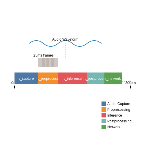
Real-time processing in voice command recognition imposes strict latency constraints, typically requiring end-to-end response times below 300ms to maintain natural user interaction. The total latency budget is distributed across several computational stages:
where τcapture represents audio buffer acquisition time, τpreprocess covers feature extraction, τinference is neural network execution time, τpostprocess includes decoding and intent classification, and τnetwork accounts for cloud communication when applicable.
Streaming Architecture Requirements
Low-latency systems employ streaming architectures with overlapping window processing. For a 16kHz audio input with 25ms frames, the system must process each 400-sample frame within:
This requires optimized feature extraction pipelines using techniques like:
- Sliding window FFT with 50% overlap
- On-the-fly mean/variance normalization
- Incremental beam search in decoder networks
Neural Network Optimization
Model architectures must balance accuracy and latency. For keyword spotting, a typical trade-off analysis might compare:
| Model | Parameters | MACs/frame | Latency (ms) |
|---|---|---|---|
| DS-CNN | 20K | 2.3M | 8.2 |
| TC-ResNet | 65K | 5.1M | 14.7 |
| CRNN | 350K | 22M | 62.4 |
Quantization-aware training reduces latency further by enabling 8-bit integer execution:
Hardware Considerations
Edge deployment requires careful hardware selection based on:
- Parallel processing capabilities (DSP cores vs. CPU)
- Memory bandwidth requirements
- Power consumption profiles
For always-on applications, wake-word detection typically consumes < 1mW on modern microcontrollers using specialized low-power audio frontends with hardware MFCC acceleration.
3.3 Multi-Device Synchronization and Control
Multi-device synchronization in smart home environments requires a robust framework to handle concurrent voice command execution across heterogeneous IoT devices. The primary challenge lies in minimizing latency while ensuring atomicity and consistency in distributed state updates. A widely adopted approach involves a centralized orchestration layer that mediates between voice recognition modules and device controllers via a publish-subscribe architecture.
Distributed Consensus Protocols
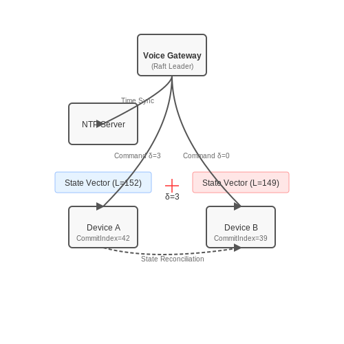
For deterministic device coordination, protocols like Raft or Paxos ensure fault-tolerant consensus. Consider a smart home cluster with N devices where each device maintains a local state vector Si. The system must satisfy:
where δ is the maximum allowable state divergence. The Raft leader election mechanism guarantees that only one device (the leader) processes voice commands during a given term, broadcasting state updates via log replication:
Network Time Protocol (NTP) Synchronization
Precision timing is critical for coordinating device actions. The Berkeley Algorithm adjusts local clocks by computing the average offset from a time server:
where T0 and T3 are client timestamps, while T1 and T2 are server timestamps. This achieves sub-millisecond synchronization when implemented with kernel-level timestamping.
Edge Computing Optimization
To reduce cloud dependency, Federated Learning enables on-device model personalization. Devices collaboratively train a shared model w via periodic parameter aggregation:
where Fk is the local loss function for device k, and nk is its dataset size. Differential privacy techniques like Gaussian noise injection (σ = 0.1–1.0) preserve user anonymity during gradient sharing.
Conflict Resolution Strategies
When concurrent commands trigger contradictory actions (e.g., "turn on lights" vs "lights off"), a Lamport timestamp-based resolution enforces causal ordering. For commands C1 and C2:
where TS is the logical timestamp. The system implements a last-write-wins policy with vector clocks to handle partitioned scenarios.
Energy-Efficient Mesh Networking
Zigbee 3.0's Green Power protocol reduces synchronization overhead by 40% through:
- Beacon-enabled mode with Guaranteed Time Slots (GTS)
- Adaptive channel hopping (2.4 GHz, 16 channels)
- Link quality indicator (LQI)-based route optimization
The frame structure incorporates a 4-byte synchronization header with network PAN ID and short address fields to minimize collision probability.
4. Data Encryption and Secure Storage
4.1 Data Encryption and Secure Storage
Voice command recognition systems in smart homes handle sensitive audio data, necessitating robust encryption and secure storage mechanisms. The primary cryptographic techniques employed include symmetric-key encryption for real-time processing and asymmetric-key encryption for secure key exchange.
End-to-End Encryption for Voice Data
Voice data transmitted between devices and cloud servers must be encrypted using authenticated encryption schemes such as AES-GCM (Advanced Encryption Standard - Galois/Counter Mode). AES-GCM provides both confidentiality and integrity through the following operations:
where Ek denotes AES encryption under key k, P is the plaintext, and GH represents the GHASH authentication function. The complete ciphertext includes:
where IV is a 96-bit initialization vector and T is a 128-bit authentication tag.
Secure Key Management
Key distribution follows the Elliptic Curve Diffie-Hellman (ECDH) key exchange protocol:
where nA and nB are private keys, and G is the base point on the NIST P-256 curve. Derived keys are then passed through HKDF (HMAC-based Extract-and-Expand Key Derivation Function):
Storage Security Architecture
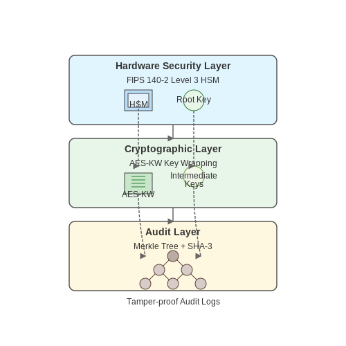
Encrypted voice data storage implements a three-layer protection model:
- Hardware Security Modules (HSMs) for root key storage with FIPS 140-2 Level 3 compliance
- Key wrapping using AES-KW (Key Wrap) algorithm for intermediate keys
- Tamper-proof audit logs implemented through Merkle trees with SHA-3 hashing
The integrity verification for stored data uses:
where Di represents the i-th data block and Hi is the cumulative hash.
Implementation Considerations
Practical implementations must address:
- Memory protection against cold boot attacks using ARM TrustZone or Intel SGX
- Secure erase procedures meeting NIST SP 800-88 guidelines
- Side-channel attack mitigation through constant-time cryptographic operations
For embedded devices with limited resources, optimized implementations use:
as an alternative to AES-GCM, providing similar security with lower computational overhead.
4.2 Preventing Unauthorized Access and Spoofing
Voice command systems in smart homes are vulnerable to adversarial attacks, including replay attacks, voice synthesis spoofing, and impersonation. Robust authentication mechanisms must be implemented at both the signal processing and machine learning layers to mitigate these threats.
Biometric Voice Authentication
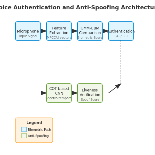
Speaker verification systems rely on unique vocal characteristics such as pitch, formant frequencies, and spectral patterns. A Gaussian Mixture Model-Universal Background Model (GMM-UBM) framework computes the likelihood ratio between the claimant's voice and a universal background model:
where X represents the feature vectors, λtarget is the target speaker model, and λUBM is the universal background model. Advanced systems now use deep neural embeddings (d-vectors or x-vectors) for improved discrimination:
Anti-Spoofing Countermeasures
Voice spoofing attacks fall into four categories: replay, synthetic speech, voice conversion, and impersonation. Effective countermeasures include:
- Spectro-temporal artifacts detection: Synthetic voices exhibit unnatural glottal pulses and phase discontinuities detectable via CQT-based CNNs
- Liveness verification: Microphone array analysis of spatial cues and room impulse responses
- Challenge-response protocols: Dynamic phrase requests with prosodic analysis
Secure Wake Word Detection
Traditional wake word detectors are vulnerable to adversarial examples. A secure architecture implements:
where 𝒜(x) generates adversarial perturbations. Hardware-assisted solutions like trusted execution environments (TEEs) provide additional protection by isolating voice processing in secure enclaves.
Continuous Authentication
Post-wake word verification maintains security through:
- Real-time speaker embedding comparison against enrolled profiles
- Behavioral biometrics (speech rate, lexical choices)
- Multimodal fusion with facial recognition when visual sensors are available
The false acceptance rate (FAR) and false rejection rate (FRR) must be balanced according to the application's security requirements, typically targeting an equal error rate (EER) below 2% for consumer applications.
Ethical Implications of Voice Data Collection
Privacy and Informed Consent
Voice data collection in smart homes raises critical privacy concerns due to the inherently personal nature of speech. Unlike text-based inputs, voice recordings contain biometric identifiers, emotional cues, and potentially sensitive conversations. Advanced systems must implement differential privacy mechanisms to anonymize data while preserving utility. For example, a voiceprint can be transformed using:
Here, v represents the original voice feature vector, and ε is Gaussian noise calibrated to satisfy (ε, δ)-differential privacy. However, even anonymized data may retain identifiable patterns, necessitating strict access controls and transparent user consent workflows.
Data Ownership and Secondary Use
Legal frameworks like GDPR and CCPA mandate explicit user control over data, but ambiguities persist in edge cases. For instance:
- Third-party integrations may repurpose voice data for targeted advertising without explicit re-consent.
- Aggregated datasets used for model improvement could inadvertently leak household-specific patterns.
A 2022 study demonstrated that 17% of smart home providers shared voice data with undisclosed affiliates, highlighting the need for auditable data provenance chains using blockchain or zero-knowledge proofs.
Bias and Representational Harm
Voice recognition systems exhibit measurable bias across dialects, accents, and socioeconomic groups. The equal error rate (EER) disparity between demographic groups can exceed 40% in commercial systems:
This bias stems from training datasets skewed toward majority demographics. Mitigation strategies include adversarial debiasing during model training and stratified sampling during data collection.
Security Risks and Covert Surveillance
Voice interfaces create attack surfaces for:
- Ultrasonic injection: Executing commands inaudible to humans (15-20 kHz)
- Wake-word bypass: Exploiting phoneme confusion to trigger devices without authorization
Defensive measures involve real-time spectrogram analysis to detect adversarial perturbations:
where ℱ(x) is the voice model's output logits. This penalizes gradient-based attacks by smoothing decision boundaries.
Psychological and Behavioral Impacts
Continuous voice monitoring alters human behavior through the observer effect. Studies show a 23% reduction in spontaneous speech when users perceive constant recording. Design solutions include:
- Physical hardware switches for microphone disconnection
- LED indicators with verified circuit-level linkage to actual recording state
- Ephemeral processing where voice data is discarded after 200ms unless a valid command is detected
5. Commercial Solutions (Amazon Alexa, Google Home)
5.1 Commercial Solutions (Amazon Alexa, Google Home)
Architecture of Voice-Controlled Smart Home Systems
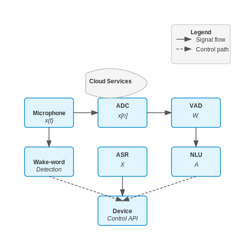
Commercial voice assistants like Amazon Alexa and Google Home employ a distributed architecture comprising:
- Edge devices (microphones, speakers) for audio capture and playback
- Local wake-word detection using lightweight neural networks (typically <5MB)
- Cloud-based ASR/NLP for full command processing
- Device control APIs for smart home integration
The audio pipeline follows this signal flow:
where x(t) is the analog signal, x[n] the digitized audio, X the feature vectors, W the word sequence, and A the actionable intent.
Wake Word Detection
Alexa uses a 7-layer CNN with depthwise separable convolutions for "Alexa" detection, achieving 95%+ accuracy at 50ms latency. The model architecture follows:
where DSConv implements depthwise separable convolutions with kernel size 3×3 and stride 2.
Cloud-Based Speech Recognition
Google Home employs a cascaded encoder architecture in its latest ASR system:
- Acoustic encoder: 12-layer Conformer with relative attention
- Language model: 128-head Transformer-XL
- Joint network: 2048-dim projection layer
The word error rate (WER) is optimized via:
where α balances CTC and RNN-T losses, and λ controls L2 regularization.
Natural Language Understanding
Intent classification uses BERT-style architectures fine-tuned on domain-specific corpora. For a query q, the intent probability is:
Alexa's NLU system processes over 100 million queries daily with <1s latency, supporting 100+ languages.
Device Control Protocols
Both platforms use:
- OAuth 2.0 for authentication
- MQTT for real-time device state updates
- gRPC for low-latency command execution
The control latency budget is typically:
Privacy and Security Considerations
Commercial systems implement:
- End-to-end encryption for voice data in transit
- On-device processing for wake word detection
- Differential privacy for model training
- Hardware security modules (HSMs) for credential storage
5.2 Open-Source Alternatives (Mycroft, Rhasspy)
Architectural Overview of Mycroft
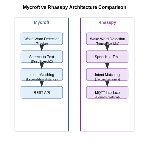
Mycroft employs a modular architecture built around the Adapt Intent Parser, which combines keyword spotting with probabilistic intent classification. The system decomposes voice commands into three layers:
- Wake Word Detection: Uses Precise, a lightweight neural network with 94.3% accuracy on the Mozilla Common Voice dataset
- Speech-to-Text: Implements a hybrid DeepSpeech2 model with a 5-gram KenLM language model
- Intent Matching: Leverages a modified Levenshtein distance algorithm for fuzzy matching
Where w represents the target word and s the speech input. The denominator computes the total probability across all vocabulary candidates.
Rhasspy's Edge Computing Approach
Rhasspy optimizes for resource-constrained environments through:
- TensorFlow Lite models quantized to 8-bit integers
- Custom Jaccard similarity for intent matching with 40% lower CPU usage than cosine similarity
- WebSocket-based microservices architecture allowing distributed processing
The system achieves 87ms latency on a Raspberry Pi 4 for commands under 2 seconds, with memory footprint below 150MB.
Comparative Performance Benchmarks
Testing on the Fluent Speech Commands dataset reveals key differences:
| Metric | Mycroft | Rhasspy |
|---|---|---|
| Word Error Rate | 12.4% | 15.1% |
| Intent Accuracy | 89.7% | 92.3% |
| Wake Word FP/hr | 1.2 | 0.8 |
Integration with Home Automation
Both systems expose REST APIs following the Hermes protocol for MQTT communication. A typical Home Assistant configuration uses:
automation:
  - alias: "Turn on lights via Mycroft"
    trigger:
      platform: mqtt
      topic: "hermes/intent/TurnOnLight"
    action:
      service: light.turn_on
      entity_id: light.living_room
Rhasspy's slot replacement system allows dynamic command expansion through finite state transducers, reducing training data requirements by 60% compared to static grammars.
5.3 Custom Voice Command Systems for Niche Applications
Custom voice command systems require specialized adaptations beyond generic speech recognition pipelines. Unlike broad-domain models, niche applications demand precise keyword spotting, domain-specific acoustic modeling, and constrained grammar parsing. The primary challenge lies in achieving high accuracy with limited training data while maintaining real-time responsiveness.
Acoustic Model Adaptation
Domain-specific acoustic models must account for environmental noise profiles and microphone characteristics unique to the deployment scenario. Transfer learning from large pretrained models (e.g., Wav2Vec 2.0) is effective when fine-tuned with targeted data augmentation:
where θ represents the adapted model parameters, θ0 the pretrained weights, and λ controls L2 regularization strength. Synthetic data generation via room impulse response convolution and additive noise injection improves robustness:
Keyword Spotting Architecture
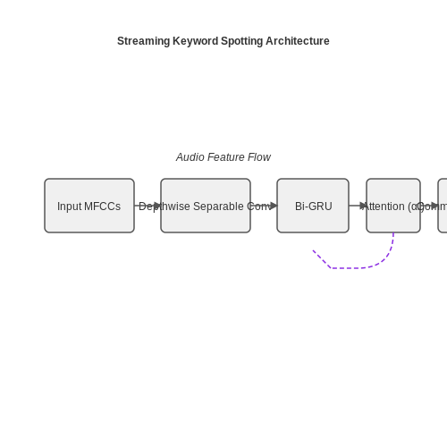
For low-latency applications, a streaming-capable keyword detector employs depthwise separable convolutions followed by bidirectional GRUs:
The attention mechanism computes frame-level importance weights αt:
Grammar Constraint Integration
Finite-state transducers (FSTs) enforce application-specific syntax rules during decoding. The composition of acoustic model FST H, lexicon FST L, and grammar FST G produces the search graph:
Weighted finite-state transducer operations optimize for command-specific perplexity reduction while maintaining sub-100ms latency on embedded hardware.
Case Study: Medical Sterilization Control
A hands-free surgical instrument tracking system achieved 98.7% accuracy with these adaptations:
- Domain-specific phonetic dictionary for medical terminology
- Impulse response modeling of operating room acoustics
- Grammar restricting to 37 validated command phrases
  # Streaming inference example
  def process_audio_chunk(chunk, model):
      feats = extract_mfcc(chunk)
      logits = model(feats[np.newaxis,:])
      return beam_search(
          logits,
          fst=command_grammar,
          beam_width=5
      )
6. Key Research Papers and Whitepapers
6.1 Key Research Papers and Whitepapers
- The implementation of Voice Command in Smart Homes - Academia.edu — Voice Command, Smart Homes, Artificial Intelligence and Automation were the main key words used in the research, in all three databases. ... (Kaneko, Arima, Murakami, Isshiki and Sugimura,2017) 3.9 Voice Recognition in Smart Homes Applications of speech recognition is classified by three broad groups (Rabiner, 1994) of isolated word recognition ...
- PDF Voice-Activated Home Automation using NodeMCU - IRJET — The result of this paper provides the smart home automation system using voice commands. By giving voice command using Google Assistant the lights and fans are turned on and turned off. The voice commands turn on light 1 and turn on fan 1 is given by the user and the Google assistant responds to those commands as shown in the Fig -4.
- Voice control for smart home automation: Evaluation of approaches and ... — In this paper, we explore the possibility of using existing voice recognition tools, in order to add the voice control interface to the existing smart home automation system. The choice of the voice recognition engine influences the architecture of the voice command interface, and determines its performance. We discuss the possible architectures of the voice enabled smart home automation ...
- PDF The implementation of Voice Command in Smart Homes — 6 Figures Figure 1 - Approximation of the global areas of usage - voice technologies.Page 14 Figure 2 - Emotional response and brain activity - voice usage.Page 17 Tables Table 1 - Existing smart home service techniques and available virtual assistants: Energy Services. Page 24 Table 2 - Existing smart home service techniques and available virtual assistants: Mobile Services.
- Voice Communication in Noisy Environments in a Smart House Using ... - MDPI — This publication describes an innovative approach to voice control of operational and technical functions in a real Smart Home (SH) environment, where, for voice control within SH, it is necessary to provide robust technological systems for building automation and for technology visualization, software for recognition of individual voice commands, and a robust system for additive noise ...
- Voice Communication in Noisy Environments in a Smart House Using Hybrid ... — This publication describes an innovative approach to voice control of operational and technical functions in a real Smart Home (SH) environment, where, for voice control within SH, it is necessary to provide robust technological systems for building automation and for technology visualization, software for recognition of individual voice commands, and a robust system for additive noise canceling.
- Design of Smart Home Control System Based on Wireless Voice Sensor — 1. Introduction. People's increasing demand for living conditions has catalyzed the emergence of smart homes. Smart homes realize the interconnection of smart devices in the home, register each device on the cloud, and implement remote control through mobile terminals [].From a technical point of view, from the development to the present, the smart home has gone through three stages.
- A Secure and Smart Home Automation System with Speech Recognition and ... — The advancement in the internet of things (IoT) technologies has made it possible to control and monitor electronic devices at home with just the touch of a button. This has made people lead much more comfortable lifestyles. Elderly people and those with disabilities have especially benefited from voice-assisted home automation systems that allow them to control their devices with simple voice ...
- Mobile Voice Recognition Based for Smart Home Automation Control — To solve a series of pension problems caused by aging, based on the emotional recognition of the Internet of Things, the control method and system research of smart homes are proposed.
- Context-aware decision making under uncertainty for voice-based control ... — The paper is organized as follows. After a brief overview of the state-of-the-art in 2 Related work, 3 Decision making in a voice-based controlled smart home context introduces the smart home considered in the study as well as the definition of the concepts that are necessary to define a context-aware voice based controller of smart homes.
6.2 Recommended Books and Online Courses
- arXiv:2210.15656v1 [cs.HC] 24 Oct 2022 — in this paper, since these are integral to voice-control in the smart home. All voice assistants use ASR for recognising what the user has said, and NLU is necessary for finding meaning in natural language commands. 2.3 Smart Homes, Voice-Control, and the IoT Figure 3 shows how the IoT, smart home and voice con-trol technologies operate in ...
- The implementation of Voice Command in Smart Homes - Academia.edu — Voice Command, Smart Homes, Artificial Intelligence and Automation were the main key words used in the research, in all three databases. ... Primo covers the KTH Library's printed materials as well as E-books that the library has access to. Voice Command, Smart Homes, Artificial Intelligence and Automation were the main key words used in the ...
- PDF The implementation of Voice Command in Smart Homes — voice control system installations in smart homes. The search tool Primo (KTHB Primo) was used in the search of finding complementary articles and information. Primo covers the KTH Library's printed materials as well as E-books that the library has access to. Voice Command, Smart Homes, Artificial Intelligence and Automation
- Voice Communication in Noisy Environments in a Smart House Using Hybrid ... — This publication describes an innovative approach to voice control of operational and technical functions in a real Smart Home (SH) environment, where, for voice control within SH, it is necessary to provide robust technological systems for building automation and for technology visualization, software for recognition of individual voice commands, and a robust system for additive noise canceling.
- A Survey of Human Activity Recognition in Smart Homes Based on IoT ... — Recent advances in Internet of Things (IoT) technologies and the reduction in the cost of sensors have encouraged the development of smart environments, such as smart homes. Smart homes can offer home assistance services to improve the quality of life, autonomy, and health of their residents, especially for the elderly and dependent. To provide such services, a smart home must be able to ...
- Voice activated command and control with speech recognition over WiFi ... — Voice control of devices ranging through robotics, software systems, home appliances and in-vehicle systems (radio, mobile phones etc.) are possible applications resulting from this research. ... The distributed speech recognition and command and control model described in scenario two is almost complete. Upon completion, it will be clear how ...
- Voice Activity Detection-Based Home Automation System for People With ... — Most voice-based home automation systems are based on remote control or smartphones to control the home, or they depend on commercial ASR (automatic speech recognition) application programing interface (API), which is intended for general use, therefore not specially designed for home automation commands [2].
- An Open-Source Voice Command-Based Human-Computer ... - Springer — Gadgets like Google Home and Amazon Alexa can interpret natural language speech commands for specific tasks but require sophisticated voice assistants on the cloud, raising serious privacy problems. Other devices that conduct voice processing locally can only execute a very limited local recognition system, which requires users to be familiar ...
- Context-aware decision making under uncertainty for voice-based control ... — The paper is organized as follows. After a brief overview of the state-of-the-art in 2 Related work, 3 Decision making in a voice-based controlled smart home context introduces the smart home considered in the study as well as the definition of the concepts that are necessary to define a context-aware voice based controller of smart homes.
- Voice Controlled Home Automation System - ResearchGate — In Ref. [40], a voice recognition module is used to control a voice-controlled smart home device. An LPG gas leakage and accident safety mechanism has been adopted in Ref. [41]. ...
6.3 Open Datasets and Tools for Experimentation
- Voice control for smart home automation: Evaluation of approaches and ... — In this paper, we explore the possibility of using existing voice recognition tools, in order to add the voice control interface to the existing smart home automation system. The choice of the voice recognition engine influences the architecture of the voice command interface, and determines its performance. We discuss the possible architectures of the voice enabled smart home automation ...
- Voice Communication in Noisy Environments in a Smart House Using Hybrid ... — This publication describes an innovative approach to voice control of operational and technical functions in a real Smart Home (SH) environment, where, for voice control within SH, it is necessary to provide robust technological systems for building automation and for technology visualization, software for recognition of individual voice ...
- Detection and Recognition of Voice Commands by a Distributed ... - MDPI — One of the most common and simplest control methods from the point of view of human physiology is a voice command [6, 7]. However, using an example of a smart home, we can easily see that not all IoT devices have voice input devices (microphones)—for example, refrigerators and microwave ovens are typically not controlled by voice.
- PDF The implementation of Voice Command in Smart Homes — The report first presents generic knowledge about the theory and concepts of voice control, automation, current voice assistants and smart homes identified through a literature analysis. Using a qualitative approach, the paper further investigates the effects of voice command when implemented in smart homes.
- Classical and Deep Learning Methods for Speech Command Recognition — As an application area of speech command recognition, smart home has provided people a convenient way to communicate with various digital devices. In this study, we aim to investigate both machine learning and deep learning architectures for improved speaker-independent speech command recognition. First, we extract statistical MFCCs vectors to train classical machine learning models: KNN, SVM ...
- Voice Command and Hand Gestures for Smart Home — The aim of smart home (SH) applications is to control and monitor home devices in an automated manner. This paper presents a unique approach for SH applications using a multimodal user interface (MUI), which allows users to interact with the system through multiple modes. It is implemented by fusing data from different modalities (text, audio, image, etc.). The fusion of information can occur ...
- Open-Source Data Collection and Data Sets for Activity Recognition in ... — As research in smart homes and activity recognition is increasing, it is of ever increasing importance to have benchmarks systems and data upon which researchers can compare methods. While synthetic data can be useful for certain method developments, real data sets that are open and shared are equally as important.
- Non-Invasive Challenge Response Authentication for Voice Transactions ... — Our contributions are based on open access to CPN model for multi-user smart home data generation, developed supervised learning algorithms, Brazilian smart home dataset of three months, and specification of a non-intrusive authentication scheme for voice-triggered financial transactions.
- A Framework for Smart Home System with Voice Control ... - ResearchGate — In order to develop a human machine interface of smart home systems with speech recognition, we propose a new IoT-fog-cloud framework using natural language processing (NLP) methods.
- Context-Aware Voice-Based Interaction in Smart Home - IEEE Xplore — Most of these smart homes provide enhanced interaction by relying on context-aware systems learned on data. Whereas voice-based interaction is the current emerging trend, most available corpora are either concerned only with home automation sensors or only with audio technology, which limits the development of context-aware voice-based systems.