

Learning from Weak Supervision
1. Definition and Key Characteristics of Weak Supervision
Definition and Key Characteristics of Weak Supervision
Weak supervision refers to a machine learning paradigm where models are trained using noisy, incomplete, or approximate labels, rather than relying on meticulously curated ground-truth annotations. Unlike traditional supervised learning, which assumes high-quality labeled data, weak supervision leverages diverse sources of imperfect supervision to reduce annotation costs while maintaining model performance.
Formal Definition
Given an input space X and output space Y, weak supervision operates under the assumption that the available labels y ∈ Y are generated through a noisy or approximate process. Let λ represent a labeling function that maps inputs to weak labels:
where ∅ denotes abstention (no label provided). The key distinction from standard supervision lies in the relaxation of label quality requirements.
Key Characteristics
Weak supervision exhibits several defining properties that differentiate it from other learning paradigms:
- Noisy Label Sources: Labels may originate from heuristic rules, distant supervision, crowd workers, or other imperfect annotation processes.
- Partial Coverage: Not all instances necessarily receive labels (∅ outputs are permitted).
- Multi-Source Integration: Multiple weak supervision sources can be combined to improve coverage and accuracy.
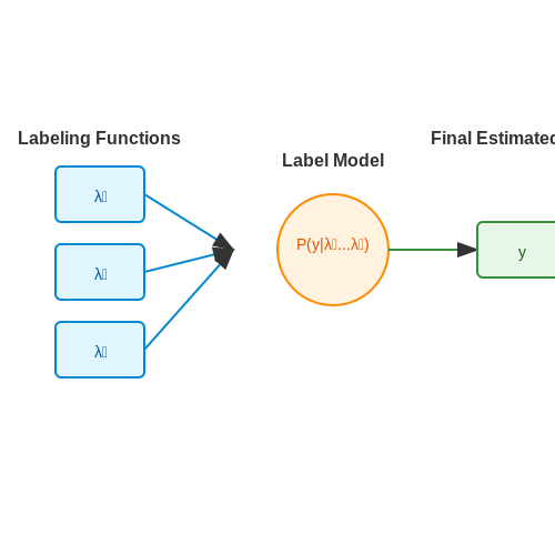
- Label Model: A probabilistic model typically reconciles conflicting or overlapping weak labels.
Mathematical Framework
The weak supervision pipeline can be formalized as a two-stage process. First, m labeling functions λ1, ..., λm generate weak labels. These are then combined through a label model that estimates the true latent label y:
The label model accounts for dependencies and accuracies of different sources. For independent sources, this simplifies to:
Practical Considerations
In real-world applications, weak supervision requires careful handling of several challenges:
- Source Reliability Estimation: Determining the accuracy and biases of each labeling function.
- Conflicting Labels: Resolving disagreements between different weak supervision sources.
- Coverage-Accuracy Tradeoff: More comprehensive labeling functions often introduce more noise.
Modern implementations often use graphical models or neural networks to learn the relationships between weak sources and true labels, with the Snorkel framework being a prominent example of this approach.
Types of Weak Supervision: Incomplete, Inexact, Inaccurate
Incomplete Supervision
Incomplete supervision arises when only a subset of training data is labeled, while the majority remains unlabeled. This scenario is common in applications like medical imaging, where expert annotations are costly. Formally, given a dataset $$D = \{(x_i, y_i)\}_{i=1}^l \cup \{x_j\}_{j=l+1}^n$$, only $$l \ll n$$ samples have labels. Techniques like semi-supervised learning leverage the unlabeled data by assuming smoothness or cluster structure in the feature space. For instance, the graph-based label propagation algorithm minimizes:
where $$W_{ij}$$ encodes similarity between samples, and $$\lambda$$ controls the trade-off between labeled and unlabeled data fidelity.
Inexact Supervision
Inexact supervision provides coarse-grained labels, such as image-level tags for object localization (e.g., "dog present" instead of bounding boxes). This is prevalent in multiple-instance learning (MIL), where a bag of instances $$B_i = \{x_{i1}, ..., x_{im}\}$$ has a label $$Y_i$$ defined as:
Deep MIL frameworks like Attention-based MIL learn instance-level weights $$\alpha_{ij}$$ to aggregate features: $$z_i = \sum_j \alpha_{ij} x_{ij}$$, where $$\alpha_{ij}$$ is computed via a neural network.
Inaccurate Supervision
Inaccurate supervision involves noisy or erroneous labels, often due to crowdsourcing or automated heuristics. The noise can be uniform (random flips) or structured (class-dependent). To model this, let $$\tilde{y}$$ be the observed noisy label and $$y^*$$ the true label. A common approach assumes a noise transition matrix $$T \in \mathbb{R}^{k \times k}$$, where $$T_{ij} = P(\tilde{y} = j \mid y^* = i)$$. Robust methods like Forward Correction adjust the loss function:
Recent work in meta-learning also optimizes the noise matrix $$T$$ jointly with model parameters.
Practical Considerations
- Incomplete supervision benefits from consistency regularization (e.g., Π-model or Mean Teacher).
- Inexact supervision requires inductive biases like spatial continuity in vision tasks.
- Inaccurate supervision demands noise-robust architectures (e.g., symmetric cross-entropy).
For example, in satellite imagery analysis, weak supervision combines incomplete (few labeled pixels), inexact (image-level land-cover tags), and inaccurate (crowdsourced labels) signals, necessitating hybrid approaches.
1.3 Comparison with Traditional Supervised Learning
Traditional supervised learning relies on high-quality, fully labeled datasets where each input x is paired with a precise ground-truth label y. The learning objective is to minimize a loss function L(f(x), y), where f represents the model's predictions. In contrast, weak supervision operates under the assumption that labels are either noisy, incomplete, or derived from heuristic rules, requiring fundamentally different optimization approaches.
Label Quality and Noise Robustness
Supervised learning assumes i.i.d. (independent and identically distributed) data with minimal label noise. Weak supervision, however, explicitly models label noise or uncertainty. For instance, if labels are provided by multiple noisy annotators, the weak supervision framework may treat the true label as a latent variable and model annotator reliability. The probability of observing a noisy label ỹ given the true label y can be expressed as:
where A_j represents the reliability of annotator j. This contrasts with supervised learning, where P(ỹ | y) is implicitly assumed to be a Dirac delta function.
Data Efficiency and Scaling
Weak supervision often leverages large amounts of weakly labeled data, whereas supervised learning requires expensive manual annotation. For example, Snorkel (Ratner et al., 2017) generates probabilistic labels via labeling functions, enabling training on millions of unlabeled examples. The trade-off is a more complex learning objective:
where R(θ) is a regularization term accounting for label uncertainty.
Model Generalization
Supervised models may overfit to clean but limited labeled data, while weakly supervised models must generalize despite label noise. Recent theoretical work (Northcutt et al., 2021) shows that weak supervision can achieve comparable asymptotic performance to supervised learning if the noise is properly characterized, with the error gap vanishing as n → ∞:
where ε depends on the noise structure.
Practical Trade-offs
- Annotation Cost: Weak supervision reduces labeling effort by 10-100x but requires domain expertise to design labeling heuristics.
- Model Complexity: Weakly supervised models often incorporate latent variable estimation or expectation-maximization, increasing computational overhead.
- Performance Ceiling: Supervised learning typically achieves higher accuracy given sufficient clean data, but weak supervision scales better to large datasets.
2. Label Propagation and Label Aggregation Techniques
Label Propagation and Label Aggregation Techniques
Weak supervision often relies on noisy or incomplete labels, requiring robust techniques to propagate and aggregate labels across datasets. Label propagation leverages the manifold structure of data to infer missing labels, while label aggregation combines multiple weak signals into a consolidated label.
Label Propagation via Graph-Based Methods
Given a dataset with partially labeled instances, label propagation operates on a graph G = (V, E), where nodes V represent data points and edges E encode pairwise similarities. The goal is to minimize the energy function:
where L denotes the set of labeled nodes, y_i are the observed labels, f_i are the predicted labels, and w_{ij} is the edge weight between nodes i and j. The parameter μ controls the trade-off between fitting observed labels and smoothness across the graph. The solution can be derived via matrix inversion or iterative updates:
where D is the degree matrix and W is the adjacency matrix. Convergence is guaranteed for connected graphs.
Label Aggregation from Multiple Weak Sources
When multiple weak labelers (e.g., heuristic rules, crowd workers) provide noisy labels, aggregation techniques estimate the true label y from weak signals {λ_1, ..., λ_m}. The Dawid-Skene model is a canonical approach, modeling each labeler’s accuracy as a confusion matrix π_j:
The true label posterior is inferred via expectation-maximization (EM), alternating between:
Variants incorporate labeler reliability, task difficulty, or dependencies between labelers.
Practical Considerations
- Graph Construction: Choice of similarity metric (e.g., RBF kernel, k-NN) critically impacts propagation quality.
- Scalability: Approximate methods like anchor graphs or Nyström approximation reduce the O(n^3) cost of exact propagation.
- Heterogeneous Noise: Robust aggregation requires modeling labeler biases (e.g., spammers, experts) and task-specific confusions.
Applications span semi-supervised learning (e.g., classifying text with few labeled examples) and crowdsourcing (e.g., aggregating medical diagnoses from multiple clinicians).

Snorkel: Programmatic Weak Supervision Framework
Snorkel is a state-of-the-art weak supervision framework that enables training machine learning models using programmatically generated noisy labels rather than hand-labeled data. Developed at Stanford, it addresses the fundamental bottleneck of supervised learning - the need for large, high-quality labeled datasets - by allowing domain experts to encode their knowledge as labeling functions (LFs) that programmatically assign labels to unannotated data.
Core Components
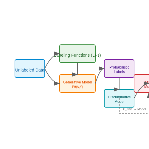
The Snorkel framework consists of three key components:
- Labeling Functions (LFs): User-defined Python functions that encode heuristics, patterns, or distant supervision signals to generate noisy labels for training data.
- Generative Model: A probabilistic graphical model that estimates the accuracy and correlations between labeling functions to produce probabilistic training labels.
- Discriminative Model: A standard machine learning model (e.g., neural network) trained on the probabilistic labels output by the generative model.
Mathematical Foundation
The generative model in Snorkel formulates the problem as estimating the true latent class label Y given the observed labeling function outputs Λ. The model assumes:
where θ represents the parameters modeling LF accuracies and correlations. The model is trained using maximum likelihood estimation:
where n is the number of data points and Λj are the labeling function outputs for the j-th data point.
Implementation Workflow
A typical Snorkel implementation follows these steps:
from snorkel.labeling import labeling_function
from snorkel.labeling.model import LabelModel

# 1. Define labeling functions
@labeling_function()
def lf_contains_keyword(x):
    return 1 if "error" in x.text.lower() else 0

@labeling_function()
def lf_from_blacklist(x):
    return 0 if x.text in blacklist else -1

# 2. Apply LFs to unlabeled data
applier = PandasLFApplier([lf_contains_keyword, lf_from_blacklist])
L_train = applier.apply(df_train)

# 3. Train generative model
label_model = LabelModel(cardinality=2)
label_model.fit(L_train)

# 4. Generate probabilistic labels
probs_train = label_model.predict_proba(L_train)

# 5. Train discriminative model
model = LogisticRegression()
model.fit(X_train, probs_train)
Advanced Features
Snorkel provides several advanced capabilities for complex weak supervision scenarios:
- Multi-task learning: Support for learning across multiple related tasks simultaneously by sharing information between them.
- Active learning: Integration with active learning to strategically query human experts for labels where the model is most uncertain.
- Transfer learning: Ability to leverage pre-trained models as labeling functions or for feature extraction.
- Data augmentation: Tools for programmatic data augmentation to increase training set diversity.
Practical Considerations
When implementing Snorkel in production systems, several factors must be considered:
- Labeling function design: LFs should have reasonable coverage and accuracy, but can be overlapping and conflicting.
- Model selection: The discriminative model architecture should match the complexity of the underlying task.
- Performance monitoring: Continuous evaluation is needed as the relationship between LFs and true labels may drift over time.
- Computational efficiency: For large datasets, distributed computation may be required for the labeling function application phase.
Empirical studies have shown Snorkel can achieve within 2-5% of fully supervised approaches while requiring orders of magnitude less hand-labeled data. In domains like medical text analysis, it has demonstrated particular success where expert labeling is expensive and time-consuming.
2.3 Weakly Supervised Deep Learning Approaches
Architectural Adaptations for Weak Supervision
Deep neural networks trained under weak supervision require architectural modifications to handle label noise, partial annotations, and incomplete supervision. Multi-task learning frameworks are commonly employed, where auxiliary tasks (e.g., pseudo-label refinement or uncertainty estimation) are jointly optimized with the primary task. The network typically consists of:
- A shared feature extractor fθ(x)
- Task-specific heads hφ(i) for each supervision signal
- A confidence estimation module gψ
where λi are task weighting coefficients and R(θ) is a regularization term. The expectation is taken over each weakly labeled dataset Di with corresponding loss ℓi.
Label Noise Robust Optimization
For noisy label scenarios, the loss function must be reformulated to prevent memorization of incorrect labels. Generalized cross-entropy (GCE) combines the benefits of mean absolute error and cross-entropy:
where q ∈ (0,1] is a hyperparameter controlling the noise robustness. When q→1, GCE becomes standard cross-entropy; when q→0, it approaches MAE.
Consistency Regularization
Weak supervision benefits from consistency constraints between different views or augmentations of the same input. Given two random augmentations x(1), x(2) of input x, the consistency loss enforces:
where d(·,·) is a distance metric (typically KL divergence for classification). This approach is particularly effective when combined with pseudo-labeling strategies.
Attention Mechanisms for Partial Labels
When only partial labels are available (e.g., image-level instead of pixel-level), attention modules can learn to focus on relevant regions. The spatial attention weights A(x) are computed as:
where σ is the sigmoid function. The final prediction combines features weighted by attention:
Multi-Instance Learning Formulation
For bag-level labels (positive if at least one instance is positive), deep MIL approaches learn instance-level classifiers with aggregation:
where g is a logistic function. Recent variants employ attention-based aggregation:

3. Weak Supervision in Natural Language Processing
Weak Supervision in Natural Language Processing
Weak supervision in NLP leverages noisy, incomplete, or heuristic-generated labels to train models when high-quality annotated data is scarce. Unlike traditional supervised learning, which relies on gold-standard labels, weak supervision combines multiple weak signals—such as pattern matching, knowledge bases, or crowd annotations—into a probabilistic training signal. This approach is particularly valuable in NLP, where manual annotation is expensive and domain expertise is often required.
Sources of Weak Supervision in NLP
Common sources of weak supervision in NLP include:
- Pattern-based labeling: Handcrafted rules or regular expressions (e.g., extracting product names using patterns like "buy [X] online").
- Distant supervision: Aligning text with structured knowledge bases (e.g., linking entity mentions to Wikidata entries).
- Crowdsourcing: Aggregating noisy labels from non-expert annotators.
- Pre-trained model predictions: Using outputs from models like BERT as silver labels.
Mathematical Framework
Given a set of weak labeling functions λ1, ..., λm, each generating noisy labels for input x, the goal is to estimate the true latent label y. The unified probabilistic model can be expressed as:
where Z is a normalization constant. The parameters are typically learned via expectation-maximization (EM), optimizing:
Advanced Techniques
Label Model Learning
Modern approaches like Snorkel model the accuracies and correlations of labeling functions. The label model estimates:
where W captures dependencies between labeling functions. This is trained via logistic regression on a small validation set.
End-to-End Weak Supervision
Frameworks like WeaSEL jointly train the label model and downstream task model, optimizing:
where y* represents any available gold labels.
Applications and Case Studies
Weak supervision has enabled NLP systems in domains with limited labeled data:
- Clinical text mining: Combining ICD-9 code heuristics with discharge summaries to train entity recognizers.
- Social media analysis: Using emoji patterns as weak sentiment labels.
- Multilingual NLP: Projecting annotations across languages via parallel corpora.
Challenges and Limitations
Key challenges include:
- Noise propagation: Systematic errors in weak signals can bias models.
- Function engineering: Creating high-coverage labeling functions requires domain knowledge.
- Long-tail distributions: Rare classes may receive insufficient weak supervision.
Computer Vision with Limited or Noisy Labels
Weak supervision in computer vision often arises from noisy, incomplete, or imprecise labeling, which can stem from crowdsourcing, heuristic rules, or automated annotation pipelines. The challenge lies in training robust models despite label imperfections, where traditional supervised learning fails due to overfitting to noise or underutilization of weakly labeled data.
Noise-Robust Loss Functions
Standard cross-entropy loss is sensitive to label noise, leading to poor generalization. Symmetric noise-robust losses, such as Generalized Cross-Entropy (GCE), mitigate this by downweighting high-confidence predictions that may correspond to noisy labels:
where pi is the predicted probability for the labeled class and q ∈ (0,1] controls the degree of noise robustness. For q → 0, GCE approximates standard cross-entropy, while q = 1 yields mean absolute error, which is theoretically robust to symmetric noise.
Co-Teaching and MentorNet
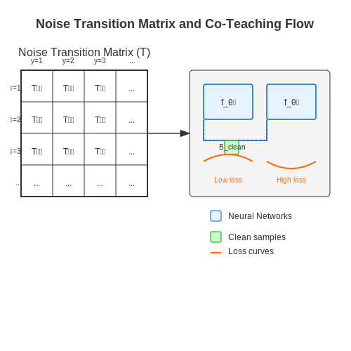
Co-teaching maintains two parallel models that iteratively select likely clean samples for each other’s training. At each batch, instances with lowest loss values are retained:
where k is a pre-defined ratio of clean samples. MentorNet extends this by learning a curriculum to weight training samples dynamically, using a meta-network that predicts sample usefulness based on historical loss patterns.
Label Noise Transition Matrix
When noise patterns are structured (e.g., class-dependent), the noise transition matrix T ∈ ℝC×C models the probability of true class j being flipped to observed class i:
Estimating T enables noise-corrected training by modifying the loss to account for probable true labels. Anchor points—identifiable clean samples per class—are often used to estimate T without explicit clean data.
Contrastive Learning with Noisy Labels
Self-supervised pretraining (e.g., SimCLR) provides noise-robust representations by maximizing agreement between augmented views of the same image. The contrastive loss for a batch of N samples is:
where z denotes projected embeddings and τ is a temperature parameter. This approach decouples feature learning from noisy labels, enabling better fine-tuning performance with limited clean data.
Uncertainty-Aware Weak Supervision
Bayesian neural networks quantify predictive uncertainty to identify potentially mislabeled samples. The epistemic uncertainty for input x is estimated via Monte Carlo dropout:
where θm are sampled dropout masks. High-uncertainty samples can be excluded or relabeled during training.
Case Study: Medical Imaging with Noisy Annotations
In pneumothorax detection from chest X-rays, radiologist disagreements lead to inherent label noise. A hybrid approach combining noise-aware loss (GCE with q = 0.7) and co-teaching improved F1-score by 14% over standard training, demonstrating the efficacy of weak supervision techniques in critical real-world applications.
Healthcare and Biomedical Data Annotation
Weak supervision in healthcare and biomedical applications addresses the challenge of obtaining high-quality labeled data when expert annotations are scarce, expensive, or time-consuming. Medical imaging, electronic health records (EHRs), and genomic datasets often exhibit complex, high-dimensional structures that require specialized annotation strategies.
Noisy Labels in Medical Imaging
Radiology reports, pathology slides, and other medical imaging data often contain inherent label noise due to inter-rater variability, ambiguous cases, or incomplete ground truth. Weak supervision frameworks model this noise probabilistically. Let Y denote the observed noisy label and Z the latent true label. The noise transition matrix T captures the probability of label corruption:
Estimating T enables correction of noisy labels during training. For instance, in chest X-ray classification, weakly supervised methods leverage multiple radiologists' annotations as noisy sources, then apply matrix completion techniques to recover the consensus.
Distant Supervision from EHRs
Electronic health records provide indirect supervision through diagnostic codes, medication orders, and clinical notes. However, these are imperfect proxies for precise phenotypic labels. A weakly supervised model for disease classification might treat ICD-10 codes as noisy labels, then incorporate temporal patterns and lab results as auxiliary signals. The learning objective combines a primary loss on noisy labels with a consistency regularization term:
where Augment(x) applies domain-specific transformations like random cropping in medical images or synonym replacement in clinical text.
Biological Sequence Annotation
Genomic and proteomic data annotation faces unique challenges due to the combinatorial explosion of possible sequences and sparse experimental validation. Weak supervision integrates:
- Evolutionary conservation scores from multiple sequence alignments
- Predicted binding affinities from biophysical models
- High-throughput screening results with varying confidence levels
The Snorkel framework has been adapted to aggregate these heterogeneous signals through learned labeling functions. For protein function prediction, each source s generates probabilistic labels λs(x), combined via a generative model:
Case Study: Weakly Supervised Tumor Segmentation
In a recent application to brain MRI segmentation, researchers used:
- Radiology reports (weak labels for tumor presence)
- Bounding boxes from clinical workflows
- Semi-synthetic data generated via tumor growth simulations
The model architecture incorporated a attention mechanism to weight the reliability of each weak source dynamically during training. Quantitative evaluation showed the approach achieved 92% of fully supervised performance while requiring only 5% of expert-annotated voxels.
Regulatory and Ethical Considerations
When deploying weakly supervised systems in clinical settings, several factors require careful attention:
- Provenance tracking for all label sources to enable auditability
- Quantification of uncertainty at both the instance and population levels
- Mechanisms to detect and correct for systematic biases in weak sources
The FDA's Software as a Medical Device (SaMD) framework now includes specific guidance for AI/ML systems using weakly labeled data, emphasizing the need for rigorous validation against held-out expert annotations.

4. Handling Label Noise and Bias
4.1 Handling Label Noise and Bias
Label Noise in Weak Supervision
Label noise arises when training data contains incorrect or imprecise annotations, a common issue in weakly supervised learning where labels are often derived from heuristics, crowd-sourcing, or distant supervision. The noise can be categorized into:
- Random noise: Errors occur uniformly across classes.
- Systematic noise: Errors correlate with specific features or label subsets.
Formally, for a dataset with true labels y and observed noisy labels ỹ, the noise can be modeled via a transition matrix T, where Tij = P(ỹ = j | y = i). Estimating T is critical for noise correction.
Bias Mitigation Strategies
Label bias occurs when annotations disproportionately represent certain classes or features due to annotator subjectivity or data collection flaws. Advanced debiasing techniques include:
- Reweighting methods: Assign instance-specific weights to balance underrepresented groups.
- Adversarial debiasing: Train a model to simultaneously predict labels while minimizing an adversary's ability to detect protected attributes.
The adversarial objective combines a primary loss Lpred and a bias-discrimination loss Ladv:
Robust Learning Algorithms
Noise-tolerant algorithms modify standard training pipelines to reduce sensitivity to label errors:
- Co-teaching: Two models iteratively select likely clean samples for each other's training.
- Generalized Cross Entropy (GCE): Replaces standard cross-entropy with a noise-robust variant:
where q ∈ (0,1] controls the robustness level. Lower q increases resistance to outliers.
Case Study: Medical Imaging with Noisy Labels
In a 2021 study on chest X-ray classification, researchers applied a noise-aware learning framework combining:
- Transition matrix estimation via anchor points
- Curriculum learning to prioritize high-confidence samples
The approach reduced error rates by 38% compared to standard training on noisy labels, demonstrating practical efficacy in high-stakes domains.
4.2 Scalability and Computational Efficiency
Weakly supervised learning methods must handle large-scale datasets efficiently, as real-world applications often involve millions of unlabeled examples with sparse or noisy annotations. The computational complexity of learning from weak supervision depends on three key factors: the label propagation mechanism, the optimization strategy, and the underlying model architecture.
Label Propagation Efficiency
Given a weakly labeled dataset with n examples and m labeling functions (LFs), the label matrix Y ∈ ℝn×m is typically sparse. Traditional label aggregation methods, such as majority voting, scale linearly with n but require quadratic memory for dense representations. Instead, sparse matrix operations can reduce the memory footprint:
where W ∈ ℝm×k is a weight matrix learned via matrix factorization or graph-based smoothing. For graph-based methods, the Laplacian eigenmap decomposition scales as O(n3) in naive implementations but can be approximated using Nyström sampling or random Fourier features:
Optimization Strategies
End-to-end training with weak supervision often involves non-convex objectives. Stochastic gradient descent (SGD) with variance reduction techniques, such as SVRG or Adam, is preferred for scalability. The gradient updates for a model fθ with weak labels can be written as:
where B is the batch size and \(\tilde{y}_i\) is the aggregated weak label. Mini-batch processing reduces memory overhead while maintaining convergence guarantees.
Model Architecture Considerations
Lightweight architectures, such as distilled neural networks or linear models with feature hashing, are often deployed in production systems. For example, a teacher-student framework can compress a large ensemble of LFs into a single model:
Recent work in data programming has shown that leveraging GPU-accelerated libraries (e.g., TensorFlow or PyTorch) for parallel LF execution can achieve 10–100× speedups over CPU-based implementations. Hybrid approaches, such as Snorkel DryBell, demonstrate scalability to billions of examples by combining weak supervision with distributed computing frameworks like Apache Spark.
Case Study: Snorkel’s Sparse LF Representation
Snorkel mitigates memory bottlenecks by representing LFs as sparse binary matrices and using incremental learning. For a dataset with 106 examples and 103 LFs, the memory usage drops from 8 GB (dense) to <100 MB (sparse CSR format). The runtime complexity for label aggregation reduces from O(nm) to O(nnz), where nnz is the number of non-zero LF outputs.
Evaluation Metrics for Weakly Supervised Models
Evaluating models trained under weak supervision presents unique challenges due to the inherent noise and incompleteness of the training labels. Traditional metrics like accuracy and F1-score may be misleading when the ground truth is partially observed or approximated. Instead, specialized metrics are required to assess model performance robustly in weakly supervised settings.
Noise-Robust Classification Metrics
When labels are noisy, precision and recall become unreliable since false positives/negatives cannot be accurately determined. The noise-adjusted precision (NAP) and noise-adjusted recall (NAR) account for estimated label noise rates:
where εFP and εFN represent the estimated probabilities of false positives and false negatives in the weak labels. These metrics require domain-specific estimation of noise rates, often through small validation sets with clean labels.
Partial Label Learning Metrics
In partial label learning where each instance is associated with multiple candidate labels, the average precision (AP) over candidate sets provides more insight than binary accuracy:
where S is the collection of candidate label sets, Si is the candidate set for instance i, and rank(l) is the model's predicted ranking of label l. This metric evaluates how well the model ranks true labels (possibly unknown) within candidate sets.
Multi-Instance Learning Evaluation
For multi-instance learning problems where labels apply to bags of instances, bag-level accuracy remains important, but instance-level AUC provides additional insight into the model's ability to discriminate individual instances:
where f(x) is the instance-level prediction score, x+ and x- are positive and negative instances respectively, and N+, N- are their counts. This metric is particularly valuable when instance-level predictions are needed despite bag-level supervision.
Confidence-Weighted Metrics
Weak supervision often produces confidence-weighted labels. The expected calibration error (ECE) measures how well the model's confidence aligns with its accuracy:
where Bm are bins partitioning the confidence space, acc(Bm) is the accuracy in bin m, and conf(Bm) is the average confidence. Well-calibrated models are crucial when weak supervision provides probabilistic labels.
Weakly Supervised Segmentation Metrics
For weakly supervised segmentation tasks with image-level labels only, region-based metrics complement pixel-wise measures. The Intersection over Union (IoU) between predicted and ground truth regions can be approximated using:
where wc are weights derived from the weak supervision signal (e.g., class activation maps) and IoUc is the IoU for class c. This approximation is necessary when pixel-level ground truth is unavailable.
Practical Considerations
When selecting evaluation metrics for weakly supervised models, consider:
- The type and quality of available validation data
- The intended use case of the model predictions
- The nature of the weak supervision signal (noisy, partial, or incomplete)
- Computational constraints on metric calculation
In practice, multiple complementary metrics often provide the most comprehensive assessment of model performance under weak supervision. The choice of metrics should align with both the learning paradigm and the end application requirements.
5. Key Research Papers and Surveys
5.1 Key Research Papers and Surveys
- PDF A Brief Introduction to Weakly Supervised Learning - NJU — process. Thus, it is desired for machine learning techniques to work with weak supervision. This article reviews some research progress of weakly supervised learning, focusing on three typical types of weak supervision: incomplete su-pervision where only a subset of training data are given with labels; inexact supervision where the training ...
- On the relative value of weak information of supervision for learning ... — In this paper, we explore the whole spectrum of labeling scenarios throughout a comprehensive empirical study on synthetic and real data. We aim to assess the contribution of the weakly labeled examples to the learning process of generative models, based on the key study of Cozman and Cohen [1] on semi-supervised learning. Following their setting, we consider Bayesian networks as generative ...
- WeakAL : Combining Active Learning and Weak Supervision - Springer — WeakAL makes use of typical AL techniques, such as a cluster query strategy, a query strategy as well as batching of samples. Therefore, in Subsect. 2.1, we give an overview of some popular query strategies, which are used in our experiments and emphasize the importance of the right batch size in Subsect. 2.2. 2.1 Active Learning Query Strategies. In this section, we shortly introduce the ...
- A Brief Introduction to Weakly Supervised Learning - ResearchGate — This article reviews some research progress of weakly supervised learning, focusing on three typical types of weak supervision: incomplete supervision where only a subset of training data are ...
- PDF WRENCH: A Comprehensive Benchmark for Weak Supervision - NeurIPS — 3Background: Weak Supervision We first give some background on weak supervision (WS) at a high level. In the WS paradigm, multiple weak supervision sources are provided which assign labels to data, which may be inaccurate, correlated, or otherwise noisy. The goal of a WS approach is the same as in supervised learning: to
- PDF Learning with Weak Supervision for Email Intent Detection — In this paper, we propose to leverage user actions as a source of weak supervision, in addition to a limited set of annotated examples, to detect intents in emails. We develop an end-to-end robust deep neural network model for email intent identification that leverages both clean an-notated data and noisy weak supervision along with a self-paced
- Weak Supervision: A Survey on Predictive Maintenance — They developed a weak supervision loss and employed a collaborative learning strategy to address data imbalances, enabling training with a small number of defect images (5-30) without pre-training. Experimental findings show that their approach attains accuracy similar to fully supervised methods on the KolektorSDD dataset.
- Snuba: Automating Weak Supervision to Label Training Data — where x i ∈ ℝ D, y * represent the primitives for a particular object and the true label, respectively. For convenience, we focus on the binary classification setting, in which y * ∈ {− 1, 1} and discuss the multi-class setting in Section 3.4.. The primitives for each datapoint x i ∈ ℝ D can be viewed as features of the data — examples include numerical features such as area or ...
- brief introduction to weakly supervised learning | National Science ... — Abstract. Supervised learning techniques construct predictive models by learning from a large number of training examples, where each training example has a label indicating its ground-truth output. Though current techniques have achieved great success, it is noteworthy that in many tasks it is difficult to get strong supervision information like fully ground-truth labels due to the high cost ...
- Weakly-supervised Semantic Segmentation with Image-level Labels: From ... — Fully supervised semantic segmentation requires a large number of labeled images for training. Unlike it, weakly supervised semantic segmentation (WSSS) uses only partial or incomplete annotations to learn the segmentation task. This makes the weakly supervised approach more feasible for real-world applications, where obtaining large amounts of fully labeled data can be prohibitively expensive ...
5.2 Open-source Tools and Libraries
- PDF Machine Learning from Weak Supervision - Massachusetts Institute of ... — I MACHINE LEARNING FROM WEAK SUPERVISION 1 Introduction 3 1.1 MachineLearning 3 1.1.1 SupervisedLearning 3 1.1.2 UnsupervisedLearning 5 1.1.3 ReinforcementLearning 6 1.2 ElementsofClassification 7 1.2.1 Classifiers 7 1.2.2 LearningCriteria 8 1.2.3 OptimizationAlgorithms 8 1.3 AspectsofMachineLearning 9 1.3.1 LogicalLearning ...
- PDF Multi-Source Domain Adaptation with Weak Supervision for Early ... - WPI — example-to-domain importance score for each source domain. Weak Supervision: To solve the limited labeled data problem in deep learning, weak supervision techniques have been developed. The weak supervision can provide an external but weak supervision signal to the model during the training. The weak supervision can be in a form of expected ...
- Learning From Multi-source Weak Supervision for Neural Text Classification — because rule-induced weak labels are often noisy and incomplete. To address these chal-lenges, we propose a model that can be learned from multiple weak supervision sources with two key components. The first component is a rule denoiser, which estimates condi-tional source reliability using a soft attention mechanism and reduces label noise by ...
- PDF Snuba: Automating Weak Supervision to Label Training Data - VLDB — points.These primitives are user-de ned and part of open source libraries [35, 49] and data models in existing weak supervision frameworks [38,58].Primitives examples in our evaluation include bag-of-words for text and bounding box attributes for images. Pruner for Diversity. To ensure that the set of heuristics
- WeakAL : Combining Active Learning and Weak Supervision - Springer — WeakAL makes use of typical AL techniques, such as a cluster query strategy, a query strategy as well as batching of samples. Therefore, in Subsect. 2.1, we give an overview of some popular query strategies, which are used in our experiments and emphasize the importance of the right batch size in Subsect. 2.2. 2.1 Active Learning Query Strategies. In this section, we shortly introduce the ...
- Snuba: Automating Weak Supervision to Label Training Data — For our collaborators using Snuba, these primitives are usually part of data models in existing weak supervision systems and open source libraries [39, 59, 36, 51]. For example, Scikit-image includes functions to extract geometric properties from segmented images . In our evaluation, we do not allow users to extend the set of primitives beyond ...
- A General Framework for Learning from Weak Supervision — At the core of GLWS is an Expectation-Maximization (EM) (Dempster et al., 1977) learning objective formulation for weak supervision, and a forward-backward algorithm (Rabiner, 1989; Graves et al., 2006) designed to solve the EM in linear time by representing arbitrary form of weak supervision as a Non-deterministic Finite Automaton (NFA) (Rabin ...
- PDF Learning with Weak Supervision for Email Intent Detection — propose to leverage user actions as a source of weak supervision, in addition to a limited set of annotated examples, to detect intents in emails. We develop an end-to-end robust deep neural network model for email intent identification that leverages both clean an-notated data and noisy weak supervision along with a self-paced learning mechanism.
- Ontology-driven weak supervision for clinical entity ... - Nature — Doing so transforms the work of using weak supervision from that of coding task-specific labeling rules to defining a target entity type and selecting ontologies with sufficient coverage for a ...
- A weakly supervised active learning framework for non-intrusive load ... — To reduce the requirement for labelled data, approaches based on semi-supervised learning have been proposed recently [37, 38, 36].A different approach to reducing the labelling effort has been proposed in [39, 40], where a weakly supervised method is demonstrated to be more effective than the semi-supervised one [].Weak supervision allows a lightened data annotation since labels are required ...
5.3 Recommended Courses and Tutorials
- PDF Machine Learning from Weak Supervision - Massachusetts Institute of ... — Contents 12.5.3 Theoretical Analysis 12.5.3.1 Realizability assumption 12.5.3.2 Summary of main results 12.5.3.3 Proofs of main results 12.5.3.4 On the convergence rate of πP 12.6 Class-Prior Estimation with Regrouping
- PDF Learning with Constraint-Based Weak Supervision — An alternative to supervised training of machine learning models is weak supervision. Weak supervision or weakly supervised learning trains with cheap, and easy to define signals that noisily label the data.
- WeakAL: Combining Active Learning and Weak Supervision — Adjacent to semi-supervised learning, weak supervision assumes that high-quality ground truth labels exist, and many noisy labels for the rest of the data. In our case, we produce high-quality data when querying the human experts, and noisy labels when using the WS.
- PDF Learning with Weak Supervision for Email Intent Detection — Application. We show that weak supervision from user interac-tion is efective in the presence of limited amount of annotated data for the task of email intent identification. This pushes the frontier on weak supervision on email-related tasks where the focus has traditionally been on training fully supervised models. Model.
- Rule-Enhanced Active Learning for Semi-Automated Weak Supervision — A major bottleneck preventing the extension of deep learning systems to new domains is the prohibitive cost of acquiring sufficient training labels. Alternatives such as weak supervision, active learning, and fine-tuning of pretrained models reduce this ...
- PDF Neural Ranking Models with Weak Supervision — To overcome this issue, in this paper, we propose to leverage large amounts of unsupervised data to infer "noisy" or "weak" labels and use that signal for learning supervised models as if we had the ground truth labels. In particular, we use classic unsupervised IR weak supervision models as a signal for training deep neural ranking models.
- PDF Snuba: Automating Weak Supervision to Label Training Data — As deep learning models are applied to increasingly diverse problems, a key bottleneck is gathering enough high-quality training labels tailored to each task. Users therefore turn to weak supervision, relying on imperfect sources of labels like pattern matching and user-de ned heuristics. Unfor-tunately, users have to design these sources for each task. This process can be time consuming and ...
- Snuba: Automating Weak Supervision to Label Training Data — The key challenge in automating weak supervision lies in replacing the human reasoning that drives heuristic development. In our collaborations with users with varying levels of machine learning expertise, we noticed that the process to develop these weak supervision sources can be fairly repetitive.
- Learning From Multi-source Weak Supervision for Neural Text Classification — The co-training design jointly models multiple weak supervision sources to learn a text classifier in an end-to-end manner. Such a co-training framework makes it possible to learn accurate deep text classifiers with-out any labeled data.
- (PDF) Improving the performance of weak supervision searches using ... — A bstract Weak supervision searches have in principle the advantages of both being able to train on experimental data and being able to learn distinctive signal properties.







