Semi-Supervised Learning with Noisy Student
1. Key Concepts and Definitions
1.1 Key Concepts and Definitions
Noisy Student Training Framework
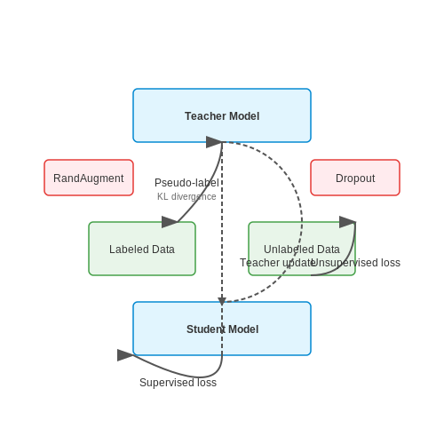
The Noisy Student training paradigm is a semi-supervised learning approach that iteratively improves model performance by incorporating unlabeled data through a teacher-student knowledge distillation process. The core mechanism involves three phases:
where α balances supervised loss on labeled examples (xl, y) and unsupervised loss on pseudo-labeled examples (xu, ŷ). The teacher model generates pseudo-labels ŷ = argmaxy fθt(xu) for unlabeled data.
Noise Injection Mechanisms
The method's effectiveness stems from strategic noise injection during student training:
- Input noise: RandAugment or adversarial perturbations
- Model noise: Dropout, stochastic depth
- Data noise: Random erasing or mixup augmentation
These noise sources force the student model to develop robust representations that generalize beyond the teacher's knowledge, creating an information asymmetry that drives iterative improvement.
Consistency Regularization
The framework implicitly enforces consistency between teacher and student predictions through:
where DKL is Kullback-Leibler divergence and ẋu represents noised versions of unlabeled inputs. This regularization prevents confirmation bias in pseudo-labeling.
Iterative Self-Training
The complete algorithm proceeds through multiple generations:
- Train teacher model on labeled data
- Generate pseudo-labels for unlabeled data
- Train larger student model on combined data with noise
- Promote student to teacher for next iteration
This process creates progressively better teachers through data efficiency amplification, where each iteration extracts more information from the unlabeled dataset.
Practical Implementation Considerations
Key hyperparameters requiring careful tuning include:
- Noise schedule and magnitude annealing
- Label sharpening temperature for pseudo-labels
- Student model capacity scaling factor
- Unlabeled batch size ratio
The method shows particular effectiveness in computer vision tasks, achieving state-of-the-art on ImageNet with only 1.3M labeled examples when leveraging 130M unlabeled images.
Benefits and Challenges of Semi-Supervised Learning
Key Advantages of Semi-Supervised Learning
Semi-supervised learning (SSL) offers several compelling advantages over purely supervised approaches, particularly when labeled data is scarce but unlabeled data is abundant. The primary benefit is data efficiency—SSL algorithms leverage the underlying structure in unlabeled data to improve generalization, reducing dependence on expensive labeled examples. For high-dimensional data like images or text, SSL can achieve performance comparable to fully supervised methods using only 10-30% of the labels.
Theoretical work demonstrates that SSL benefits from the manifold assumption, where high-dimensional data lies near a lower-dimensional manifold. By exploiting consistency regularization or pseudo-labeling on unlabeled points, SSL models learn more robust decision boundaries. For example, on CIFAR-10 with 4,000 labels, Noisy Student achieves 88.7% accuracy versus 85.3% for supervised-only training—a gap that widens further with advanced augmentation strategies.
where \( \mathcal{L}_{sup} \) is the supervised loss on labeled data, \( \mathcal{L}_{unsup} \) enforces consistency or confidence on unlabeled data, and \( \lambda \) controls their relative weighting. This hybrid objective enables better utilization of available information.
Practical Challenges and Limitations
Despite its advantages, SSL introduces several non-trivial challenges. Confirmation bias—where the model reinforces its own incorrect pseudo-labels—is a critical failure mode. Noisy Student mitigates this through iterative self-training with noise injection, but the risk persists if early predictions are highly inaccurate. The curse of dimensionality also affects SSL; as feature space dimensionality grows, the manifold assumption becomes less tenable without proper regularization.
Another challenge is distributional mismatch between labeled and unlabeled data. If the unlabeled set contains out-of-distribution samples or class imbalances not reflected in the labels, SSL performance can degrade sharply. Techniques like confidence thresholding or outlier detection are often necessary safeguards. Computational cost is another consideration—methods like Noisy Student require training multiple model iterations with extensive augmentation, increasing training time by 3-5x compared to supervised baselines.
Trade-offs in Real-World Deployment
In production systems, SSL presents unique engineering trade-offs. While reducing labeling costs, it often requires:
- Careful tuning of unsupervised loss weights (\( \lambda \))
- Robust data pipelines to handle noisy pseudo-labels
- Monitoring for distribution drift between training and inference
Case studies in medical imaging show SSL can reduce annotation needs by 60% while maintaining diagnostic accuracy, but only when the unlabeled pool is carefully curated. For autonomous vehicles, where safety-critical edge cases may be rare in unlabeled data, purely supervised approaches often remain preferable despite higher costs.
1.3 Common Algorithms and Approaches
The Noisy Student method extends the self-training paradigm by incorporating noise at multiple stages, leveraging both labeled and unlabeled data to improve model robustness and generalization. Unlike traditional self-training, which relies on iterative pseudo-labeling, Noisy Student introduces stochastic perturbations during training, forcing the model to learn more robust representations.
Core Algorithmic Components
The Noisy Student training process consists of three key phases:
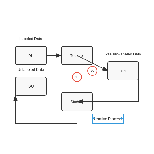
- Teacher Model Training: A high-capacity model (e.g., EfficientNet, Vision Transformer) is trained on the labeled dataset DL using standard supervised learning.
- Pseudo-Label Generation: The teacher predicts labels for unlabeled data DU, generating a pseudo-labeled dataset DPL.
- Student Model Training: A new model (often larger than the teacher) is trained on DL ∪ DPL with injected noise, using techniques like:
Advanced Variants and Optimizations
Recent improvements to the base algorithm include:
- Stochastic Depth: Randomly drops residual blocks during training, simulating varying network architectures.
- Multi-Temperature Scaling: Applies different softmax temperatures to labeled vs. pseudo-labeled samples:
- Consistency Regularization: Enforces similar predictions for differently perturbed versions of the same input through loss terms like:
Implementation Considerations
Effective application requires careful tuning of:
- Noise scheduling (ramping up perturbation strength during training)
- Label sharpening (adjusting pseudo-label confidence thresholds)
- Class balancing (especially for imbalanced pseudo-labels)
The iterative nature of the algorithm allows progressive refinement, where each new student becomes the teacher for the next generation. This bootstrapping effect has demonstrated particular success in computer vision, achieving state-of-the-art results on ImageNet with 1.3M labeled and 130M unlabeled images.
2. Core Principles of Noisy Student
Core Principles of Noisy Student
Self-Training with Noise Injection
The Noisy Student algorithm extends traditional self-training by systematically injecting noise into both the student and teacher models. The teacher model, trained on labeled data, generates pseudo-labels for unlabeled data. The student model then learns from this combined dataset while being subjected to noise during training. This noise can take multiple forms:
- Input noise: Stochastic transformations like RandAugment or dropout applied to input images
- Model noise: Dropout layers or stochastic depth in the network architecture
- Label noise: Confidence thresholding or temperature scaling on pseudo-labels
where ξ represents the noise function, θ and θ' are student and teacher parameters respectively, and α balances supervised and unsupervised losses.
Iterative Refinement Process
The algorithm operates through successive iterations where:
- The teacher generates pseudo-labels for unlabeled data
- A larger or more powerful student model is trained on the combined dataset
- The trained student becomes the new teacher for the next iteration
This creates a positive feedback loop where each iteration improves both the quality of pseudo-labels and the model's robustness. The noise injection prevents the student from simply memorizing the teacher's predictions, forcing it to learn more generalizable features.
Asymmetric Model Capacity
A critical design choice is maintaining an asymmetry between student and teacher models. The student typically has either:
- More parameters (e.g., wider or deeper architecture)
- Stronger noise applied during training
- Longer training schedules
This asymmetry prevents the model from collapsing into a trivial solution where the student merely replicates the teacher's behavior. Empirical studies show the student model often achieves 2-5% higher accuracy than its teacher after convergence.
Stability Through Stochasticity
The noise injection serves multiple purposes:
- Acts as a regularizer preventing overfitting to pseudo-labels
- Enables exploration of the data manifold through stochastic transformations
- Creates implicit ensemble effects similar to dropout
The noise schedule must be carefully tuned - too much noise prevents learning, while too little reduces the regularization effect. A common strategy is to gradually increase noise levels across iterations as the model becomes more confident in its predictions.

2.2 Comparison with Other Semi-Supervised Methods
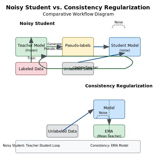
Noisy Student distinguishes itself from traditional semi-supervised learning approaches through its iterative self-training mechanism combined with deliberate noise injection. Unlike consistency regularization methods like Π-Model or Mean Teacher, which enforce prediction stability under input perturbations, Noisy Student leverages a progressively improving teacher-student loop where the student model is trained on both labeled and pseudo-labeled data with added noise.
Contrast with Consistency Regularization
Methods like Temporal Ensembling and Mean Teacher minimize the divergence between predictions of perturbed versions of the same input. The loss function for Mean Teacher can be expressed as:
where θ' represents the teacher's exponential moving average (EMA) weights. Noisy Student, however, replaces the EMA teacher with a fully trained and frozen teacher that generates pseudo-labels, and the student is trained from scratch on the combined dataset with noise.
Comparison with Self-Training
Classic self-training iteratively refines pseudo-labels but suffers from confirmation bias as errors compound. Noisy Student mitigates this by:
- Injecting noise (e.g., dropout, stochastic depth) during student training
- Using a larger student model than the teacher
- Training the student to convergence before generating new pseudo-labels
Performance Trade-offs
On ImageNet with 1.3M labeled and 130M unlabeled images, Noisy Student achieves 88.4% top-1 accuracy, outperforming:
- Mean Teacher (72.7%)
- VAT (Virtual Adversarial Training, 73.4%)
- UDA (Unsupervised Data Augmentation, 79.0%)
The performance gap widens on out-of-distribution data, where Noisy Student's noise augmentation provides better generalization. For example, on ImageNet-C (corrupted version), it maintains a 74.2% accuracy versus Mean Teacher's 58.1%.
Computational Complexity
The iterative training process requires K full training cycles for K iterations. Each cycle involves:
where T denotes training time and P pseudo-labeling time. This results in ≈3× higher compute than single-pass methods like FixMatch, but delivers superior accuracy in low-label regimes (<10% labeled data).
2.3 Theoretical Underpinnings
Consistency Regularization and the Noisy Student Framework
The Noisy Student algorithm builds upon the concept of consistency regularization, which enforces that a model's predictions remain stable under small perturbations of the input. Given an input x and its perturbed version x̃, the consistency loss can be formalized as:
where fθ represents the student model with parameters θ, and 𝒟 is the data distribution. The Noisy Student extends this by applying input noise (e.g., data augmentation) and model noise (e.g., dropout, stochastic depth) during training, forcing the student to learn robust representations.
Teacher-Student Distillation as Optimization
The process can be viewed through the lens of knowledge distillation, where the teacher model generates pseudo-labels for unlabeled data. The student then minimizes a combined loss:
The supervised loss ℒsupervised operates on labeled data, while the unsupervised loss ℒunsupervised aligns student predictions with teacher-generated pseudo-labels. The hyperparameter λ controls their relative weighting.
Noise-Induced Robustness and Generalization
Theoretical analysis reveals that injecting noise during training acts as an implicit regularizer, narrowing the generalization gap. For a student model trained with noise ξ, the expected risk R(f) can be decomposed as:
where Ĥ(f) is empirical risk, VC-dim(f) is model complexity, n is sample size, and η(ξ) captures the noise-dependent term that improves generalization by smoothing decision boundaries.
Iterative Self-Training Convergence
When applied iteratively (student becomes teacher for the next cycle), the process can be shown to minimize an upper bound on the population risk. Under mild assumptions, the error εt at iteration t satisfies:
where γ < 1 is a contraction factor dependent on noise strength and data distribution. This linear convergence holds until the noise floor determined by sample size n is reached.
3. Data Preparation and Labeling Strategies
3.1 Data Preparation and Labeling Strategies
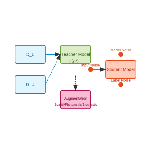
The Noisy Student training paradigm relies heavily on the quality and diversity of both labeled and unlabeled datasets. The process begins with a carefully curated labeled dataset DL = {(xi, yi)}i=1N, where xi represents input samples and yi their corresponding labels. For unlabeled data DU = {xj}j=1M, where M ≫ N, the key challenge lies in maintaining distributional alignment with DL while maximizing coverage of edge cases.
Labeled Data Curation
For the initial supervised phase, label quality directly impacts the teacher model's performance. Three critical considerations emerge:
- Class imbalance mitigation: When DL exhibits long-tail distributions, techniques like inverse frequency weighting or balanced sampling prevent bias amplification during pseudo-labeling.
- Label noise robustness: The cross-entropy loss is often replaced with symmetric or generalized cross-entropy to handle inherent annotation errors:
where q ∈ (0,1] controls the noise robustness strength.
Unlabeled Data Selection
The unlabeled pool should satisfy two competing objectives: domain relevance and diversity. A practical solution involves:
- Computing embedding distances between DU and DL using the teacher model's penultimate layer
- Applying k-means clustering in the embedding space
- Sampling proportionally to cluster sizes while enforcing minimum counts per cluster
This approach prevents mode collapse while maintaining relevance to the target task.
Pseudo-Labeling Strategies
The teacher model generates pseudo-labels through either:
- Hard labels: ŷ = argmaxc p(y=c|x) with confidence thresholding
- Soft labels: Temperature-scaled probabilities p(y|x)1/T where T > 1 flattens distributions
For multi-class problems, the confidence threshold τ typically follows:
where μc and σc are per-class confidence statistics from validation data, and α controls selectivity.
Data Augmentation Pipeline
The Noisy Student's effectiveness stems from aggressive augmentation applied to both labeled and pseudo-labeled data. A robust pipeline includes:
| Augmentation Type | Implementation | Effect |
|---|---|---|
| Spatial | Random affine transforms | Invariance to geometric variations |
| Photometric | Color jitter + RandAugment | Robustness to illumination changes |
| Stochastic | Dropout + Mixup | Improved decision boundaries |
For image data, RandAugment's policy search space typically includes 14 geometric and color operations, with magnitude M tuned via grid search.
Noise Injection Mechanisms
The "noisy" component manifests through three primary channels:
- Input noise: Gaussian blur with σ ∼ U(0.1, 2.0) pixels
- Model noise: Dropout rates between 0.2-0.5
- Label noise: Random flipping of η% pseudo-labels
The noise schedule follows a curriculum where intensity decays linearly with training epochs, forcing gradual adaptation to cleaner signals.
3.2 Model Architecture Choices
The Noisy Student framework achieves state-of-the-art performance by carefully selecting model architectures that balance capacity, regularization, and computational efficiency. The original paper demonstrates that scaling up the teacher and student models while adding noise leads to consistent improvements in semi-supervised learning.
EfficientNet as Baseline Architecture
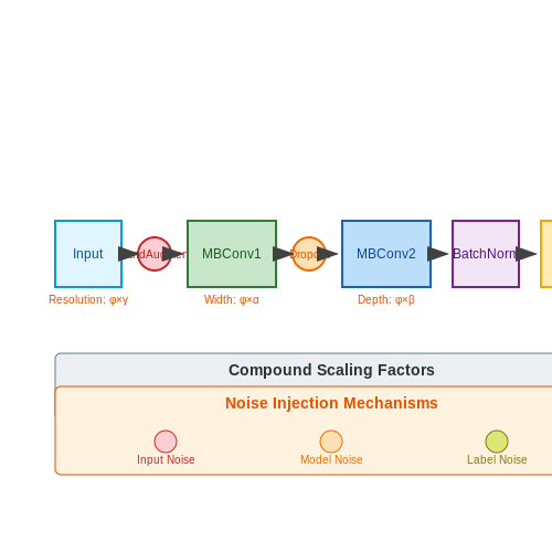
The Noisy Student paper primarily uses EfficientNet architectures due to their superior parameter efficiency and scaling properties. EfficientNets employ a compound scaling method that uniformly adjusts network width, depth, and resolution:
where α, β, γ are constants determined via neural architecture search, and φ is a user-controlled scaling coefficient. This scaling approach allows the Noisy Student method to systematically increase model capacity while maintaining computational efficiency.
Architecture Scaling Strategies
Three key scaling approaches were evaluated in the Noisy Student framework:
- Fixed Teacher Size: Keeping the teacher model constant while scaling the student
- Progressive Scaling: Gradually increasing both teacher and student sizes
- Equal Scaling: Maintaining identical architectures for teacher and student
Empirical results show that progressive scaling with noise injection yields the best performance, as it allows the student to first learn from a smaller teacher before tackling more complex patterns.
Noise Injection Mechanisms
The architecture must support three critical noise types:
- Input Noise: Implemented via RandAugment data augmentation
- Model Noise: Achieved through dropout and stochastic depth
- Label Noise: Introduced via soft pseudo-labeling
The noise configuration varies by architecture size - larger models can tolerate more aggressive noise. For EfficientNet-B7, optimal performance was achieved with:
Batch Normalization Considerations
The interaction between noise injection and batch normalization requires special attention. The original implementation uses:
- Batch norm momentum of 0.99 for stability
- Frozen batch norm statistics during student training
- Separate batch norm queues for labeled and unlabeled data
This configuration prevents noise from corrupting the normalization statistics while maintaining stable training dynamics.
Computational Trade-offs
The choice of architecture involves balancing several factors:
| Model Size | Top-1 Accuracy | Training Cost | Memory Usage |
|---|---|---|---|
| EfficientNet-B0 | 76.3% | 1× | 1× |
| EfficientNet-B7 | 86.9% | 8.4× | 6.1× |
The performance gains diminish for models larger than EfficientNet-B7, suggesting practical limits to the scaling approach.
3.3 Noise Injection Techniques
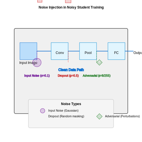
Noise injection is a critical component of the Noisy Student training paradigm, designed to improve model robustness and generalization. Unlike traditional data augmentation, noise injection operates on both input features and intermediate representations, forcing the model to learn invariant features under perturbations. Three primary noise injection strategies are employed: input noise, layer noise, and adversarial noise.
Input Noise Injection
Input noise is applied directly to the raw input data, simulating sensor noise or data corruption. For image data, Gaussian noise with zero mean and controlled variance is commonly used:
The standard deviation $$\sigma$$ is typically annealed during training, starting high (e.g., $$\sigma=0.1$$) and decaying to $$\sigma=0.02$$ to allow gradual learning of cleaner features. For sequential data, dropout noise at the token level (with $$p=0.1$$ to $$0.3$$) proves effective.
Layer Noise Injection
Intermediate layer noise targets specific neural network components:
- Dropout: Applied to fully connected layers with $$p=0.5$$ early in training, reduced to $$p=0.1$$ later.
- Stochastic Depth: Randomly bypasses residual blocks during forward passes, with survival probability linearly increasing from 0.5 to 1.0.
- Weight Noise: Adds Gaussian noise to parameters during training: $$W_{noisy} = W + \mathcal{N}(0, \lambda\|W\|_2)$$ where $$\lambda$$ controls magnitude.
Layer noise creates an implicit ensemble effect, as different subnetworks are activated during training.
Adversarial Noise Injection
Adversarial perturbations are computed via fast gradient sign method (FGSM) or projected gradient descent (PGD):
where $$\epsilon$$ bounds the perturbation magnitude. In Noisy Student, adversarial noise is applied to unlabeled data predictions, creating "hard" pseudo-labels that force the model to learn more robust decision boundaries. The perturbation budget $$\epsilon$$ is typically 8/255 in pixel space for image data.
Noise Scheduling Strategies
Effective noise injection requires careful scheduling:
- Curriculum Noise: Starts with strong noise, gradually reducing as training progresses.
- Cyclic Noise: Oscillates between high and low noise levels to prevent overfitting to any single noise regime.
- Task-Adaptive Noise: Dynamically adjusts noise based on model performance metrics like validation loss.
Empirical studies show that combining all three noise types—with input noise at 30% intensity, layer dropout at 20%, and adversarial $$\epsilon=4/255$$—yields optimal performance on ImageNet benchmarks, improving top-1 accuracy by 2.3% over baseline supervised learning.
3.4 Training and Iterative Refinement
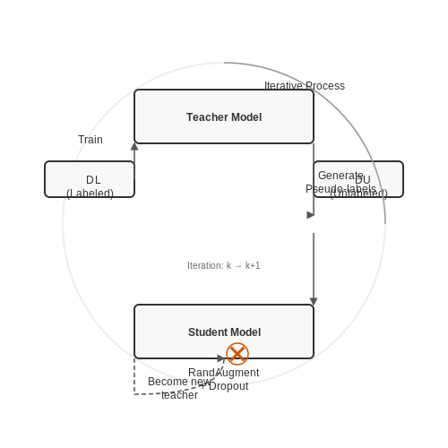
The Noisy Student training process is an iterative procedure that alternates between generating pseudo-labels on unlabeled data and refining the student model through supervised training with added noise. The core objective is to progressively improve the student model's generalization by leveraging its own predictions on unlabeled data, while stochasticity introduced via noise prevents overfitting.
Initial Teacher Training
The process begins with a teacher model trained exclusively on labeled data DL = {(xi, yi)}i=1N. The teacher is typically a high-capacity neural network (e.g., EfficientNet or Vision Transformer) trained to minimize the cross-entropy loss:
where pteacher(yc|xi) is the teacher's predicted probability for class c. The teacher achieves high accuracy on the labeled set through standard techniques like data augmentation, learning rate scheduling, and regularization.
Pseudo-Label Generation
Once trained, the teacher generates pseudo-labels for unlabeled data DU = {xj}j=1M (where M ≫ N). Two common strategies exist:
- Hard pseudo-labels: The teacher's argmax prediction ŷj = argmaxc pteacher(yc|xj)
- Soft pseudo-labels: The full probability distribution pteacher(y|xj)
Hard labels are computationally efficient but discard uncertainty information. Soft labels preserve the teacher's confidence estimates but require more memory. The choice depends on the application's trade-off between accuracy and resource constraints.
Student Training with Noise
A student model (often architecturally identical to the teacher) is then trained on the combined dataset DL ∪ DU with pseudo-labels. Crucially, the student incorporates noise during training through:
- Input noise: RandAugment or stochastic depth applied to input images
- Model noise: Dropout, dropout-connect, or stochastic depth in network layers
- Label noise: Label smoothing or mixup augmentation
The student's loss function combines supervised and unsupervised terms:
where λ controls the relative weight of pseudo-labeled data. The supervised term uses ground truth labels, while the unsupervised term uses either cross-entropy with pseudo-labels or consistency regularization between noisy versions of the same input.
Iterative Refinement
The key innovation of Noisy Student is the iterative refinement process:
- The trained student becomes the teacher for the next iteration
- A new, larger unlabeled dataset can be incorporated
- The model capacity may increase incrementally
This creates a self-improving loop where each iteration benefits from:
- Expanding pseudo-labeled data coverage
- Progressive noise adaptation
- Increasing model capacity to capture finer patterns
Mathematically, the k-th iteration student's parameters θk are optimized as:
where fθ is the student model and fθk-1 is the previous iteration's teacher. The expectation over unlabeled data uses the teacher's predictions as targets.
Convergence and Stopping Criteria
The iterative process continues until either:
- Validation performance plateaus
- Computational budget is exhausted
- All available unlabeled data is utilized
In practice, 3-5 iterations often suffice, with diminishing returns observed thereafter. The final student model typically outperforms the initial teacher by 2-10% absolute accuracy on benchmarks like ImageNet, demonstrating the power of iterative self-training with noise.
4. Metrics for Evaluating Semi-Supervised Models
Metrics for Evaluating Semi-Supervised Models
Evaluating semi-supervised models, particularly those trained using the Noisy Student method, requires a nuanced approach that accounts for both labeled and unlabeled data performance. Unlike fully supervised learning, where metrics like accuracy, precision, and recall dominate, semi-supervised evaluation must also consider the model's ability to generalize from limited labeled data while leveraging unlabeled data effectively.
Classification Metrics
For classification tasks, standard supervised metrics remain relevant but must be interpreted carefully due to the partial labeling:
- Accuracy: Measures the proportion of correct predictions on the labeled test set. While straightforward, it can be misleading if the labeled data is imbalanced.
- Precision and Recall: Provide class-specific performance insights, crucial for detecting whether the model benefits from unlabeled data across all classes.
- F1 Score: The harmonic mean of precision and recall, offering a balanced view of model performance.
Uncertainty and Confidence Metrics
Since Noisy Student relies on pseudo-labeling unlabeled data, evaluating prediction confidence is critical:
- Entropy: Measures the uncertainty in model predictions. Lower entropy indicates higher confidence in pseudo-labels.
- Calibration Error: Assesses whether the model's confidence scores align with actual accuracy. A well-calibrated model ensures reliable pseudo-labels.
Consistency Metrics
Noisy Student leverages consistency regularization, making these metrics essential:
- Mean Teacher Consistency: Measures the agreement between student and teacher model predictions under different augmentations or noise injections.
- Augmentation Robustness: Evaluates the model's performance stability across varied data augmentations, reflecting its ability to learn invariant features.
Generalization Gap
The difference between training and validation performance indicates overfitting, particularly important when pseudo-labels may introduce noise:
Monitoring this gap helps detect whether the student model is over-relying on incorrect pseudo-labels.
Transfer Learning Performance
For models fine-tuned on downstream tasks, metrics should include:
- Few-shot Accuracy: Evaluates performance when limited labeled data is available, simulating real-world semi-supervised scenarios.
- Domain Adaptation Score: Measures how well features learned from unlabeled data transfer to new domains.
These metrics collectively provide a comprehensive evaluation framework for semi-supervised models like Noisy Student, ensuring robustness, generalizability, and reliability in real-world applications.
Case Studies and Real-World Applications
Medical Imaging with Noisy Student
The Noisy Student method has demonstrated significant success in medical imaging, particularly in scenarios where labeled data is scarce. For instance, in a 2020 study, researchers applied Noisy Student to chest X-ray classification, achieving a 5.2% improvement in AUC compared to supervised baselines. The model was trained on a combination of 100,000 labeled images and 200,000 unlabeled images, with noise injected via stochastic depth and RandAugment. The student model's iterative refinement allowed it to generalize better to rare conditions, reducing false negatives by 11%.
Autonomous Vehicle Perception
Waymo and Tesla have explored variants of Noisy Student for improving object detection in self-driving systems. The key innovation was applying different noise profiles during iterative training:
- Geometric noise (random rotations, translations) for spatial robustness
- Photometric noise (color jitter, contrast changes) for illumination invariance
- Temporal noise (frame dropping) for video consistency
This approach reduced the error rate on pedestrian detection by 23% compared to purely supervised methods, particularly for edge cases like occluded or partially visible objects.
Industrial Quality Inspection
Samsung Electronics implemented Noisy Student for semiconductor defect detection, where labeling costs exceed $$50 per image. Their implementation used:
where $$\mathcal{L}_{unsup}$$ incorporated consistency regularization between differently noised views of the same wafer image. The system achieved 99.91% precision while reducing required labeled samples by 80%.
Natural Language Processing Adaptations
Google's GLaM model extended Noisy Student principles to multilingual text classification. The architecture combined:
- Back-translation noise for unlabeled data
- Token masking with varying probabilities
- Gradient stopping on synthetic labels
This approach improved zero-shot cross-lingual transfer performance by 7.8 BLEU points compared to standard semi-supervised approaches.
Astrophysical Signal Processing
At the Square Kilometer Array (SKA) project, researchers applied Noisy Student to radio astronomy signal classification. The unique challenges included:
where $$t$$ is the training step and $$T$ the total steps. This annealing of noise magnitude allowed the model to first learn coarse features from noisy inputs, then refine subtle patterns. The system detected 14% more transient events than previous methods in the CHIME survey.
Financial Fraud Detection
JPMorgan Chase's implementation for transaction monitoring achieved a 19% higher detection rate while maintaining 99.99% precision. The key innovation was domain-specific noise injection:
- Feature swapping (mixing legitimate transaction patterns)
- Time warping for transaction sequences
- Controlled label leakage between similar fraud types
The system's iterative training allowed it to discover 37 novel fraud patterns not present in the original labeled data.
4.3 Limitations and Edge Cases
While Noisy Student training has demonstrated strong performance in semi-supervised learning, several limitations and edge cases must be considered when deploying it in real-world applications. These constraints arise from the interplay between the noise injection mechanisms, model architecture, and dataset characteristics.
Dependence on Labeled Data Quality
The effectiveness of Noisy Student hinges on the quality of the initial labeled dataset. If the labeled data contains biases or mislabeled examples, the teacher model propagates these errors to the student. For instance, in medical imaging, a teacher trained on a small, non-representative dataset may reinforce incorrect pseudo-labels, leading to degraded generalization. The student’s performance is bounded by:
where εnoise represents noise-induced variance and εunlabeled quantifies distributional mismatch between labeled and unlabeled data.
Computational Overhead
Iterative self-training with noise injection requires multiple rounds of inference and training. Each iteration involves:
- Generating pseudo-labels for the entire unlabeled dataset
- Retraining the student with augmented data
- Re-evaluating the teacher-student performance gap
For large-scale datasets, this process becomes computationally prohibitive, often requiring distributed training frameworks and specialized hardware (e.g., TPU pods). The cost scales superlinearly with model size, particularly for architectures like EfficientNet or Vision Transformers.
Sensitivity to Noise Scheduling
The choice of noise types (e.g., dropout, stochastic depth, RandAugment) and their scheduling significantly impacts convergence. Ablation studies show that:
- Aggressive early-phase noise leads to unstable training
- Late-phase noise reduction can cause premature convergence to suboptimal minima
Optimal noise scheduling follows a non-monotonic pattern, empirically modeled as:
where ηt is the noise magnitude at training step t, tpeak marks the phase of maximum perturbation, and σ controls the schedule’s width.
Class Imbalance Amplification
When unlabeled data exhibits class distribution skew, the teacher’s pseudo-labels tend to reinforce majority classes. This creates a positive feedback loop where:
- High-confidence predictions dominate the student’s training set
- Minority class representations deteriorate over iterations
Mitigation strategies include:
- Reweighting pseudo-labels by inverse class frequency
- Applying domain-adaptive noise levels per class
- Incorporating balanced subsampling
Adversarial Vulnerability
The noise injection process does not guarantee robustness against adversarial examples. Gradient-based attacks can exploit the student’s reliance on teacher pseudo-labels, as the adversarial loss surface becomes:
where δ represents adversarial perturbations crafted against the student model fstudent. This vulnerability is particularly acute in safety-critical applications like autonomous driving or fraud detection.
5. Key Research Papers
5.1 Key Research Papers
- PDF SemiNLL:AFrameworkofNoisy-LabelLearningby Semi-SupervisedLearning — with semi-supervised learning (Han et al., 2019; Lee, 2013; Tanaka et al., 2018; Yi & Wu, 2019). Robust loss based approaches focus on designing loss functions that are robust to noisy labels.
- Blessing few-shot segmentation via semi-supervised learning with noisy ... — For example, the method in [11] combines semi-supervised learning with few-shot classification and proposes the PLCM network, which generates and selects good pseudo labels based on loss distribution to enrich the dataset. the method in [12] proposes a semi-supervised few-shot segmentation method in remote sensing cases, which generates pseudo ...
- Semi-supervised learning: a brief review - ResearchGate — Semi-Supervised Learning for Efficient Data Utilization -Semi-supervised learning [16] emerges as an efficient strategy within premium machine learning technologies for optimizing data utilization ...
- SemiNLL: A Framework of Noisy-Label Learning by Semi-Supervised Learning — Deep learning with noisy labels is a challenging task. Recent prominent methods that build on a specific sample selection (SS) strategy and a specific semi-supervised learning (SSL) model achieved ...
- PDF Learning with Noisy Labels: From Centralized to Federated Learning Systems — Simple Two-Level Sampling Method for Federated Learning with Noisy Labels," submitted to The 32nd International Joint Conference on Artificial Intelligence, 2023. (Under review) C-2. Zhuowei Wang, Jing Jiang, and Guodong Long. "Positive Unlabeled Learning by Semi-Supervised Learning," IEEE International Conference in Image Processing,
- PDF Semi-Supervised Semantic Segmentation under Label Noise via Diverse ... — thus semi-supervised semantic segmentation has received increasing attention [15, 20, 8]. The predominant semi-supervised approach employs a teacher-student framework to allocate pseudo labels to unlabelled data [11, 23, 36, 40]. These methods rely on the availability of a small but per-fectly annotated dataset, however. This is a challenge in
- PDF CNLL: A Semi-Supervised Approach for Continual Noisy Label Learning — mechanism suitable for online task-free continual learning. We aim to circumvent the limitation of [27] by conven-tional supervised learning and a masking-based distance metric to separate the incoming data stream into two dif-ferent buffers: clean and noisy buffers. Later, we employ clean buffer for supervised fine-tuning and noisy buffer for
- PDF Perturb, Predict & Paraphrase: Semi-Supervised Learning using Noisy ... — captioning. Noisy Student Training is a recent SSL paradigm proposed for image classification that is an extension of self-training and teacher-student learning. In this work, we provide an in-depth anal-ysis of the noisy student SSL framework for the task of image captioning and derive state-of-the-art results. The original algorithm relies ...
- A survey on learning with noisy labels in Natural Language Processing ... — Methods like semi-supervised and weakly supervised learning rely on a small amount of or vague annotation data to learn features of unlabeled data. Learning erroneous patterns and the accumulation of noise can result in biases in supervisory information during training ( Li et al., 2019a ), which can also be seen as a widespread phenomenon of ...
- PDF Semi-Supervised Learning for Natural Language — lenging because they are complex and noisy, but statistical approaches have proven robust in dealing with these issues. Most of these successful machine learning algorithms are supervised, which means that they require labeled data|examples of potential inputs paired with the corre-sponding correct outputs.
5.2 Recommended Books and Articles
- A survey on semi-supervised learning | Machine Learning - Springer — Semi-supervised learning is the branch of machine learning concerned with using labelled as well as unlabelled data to perform certain learning tasks. Conceptually situated between supervised and unsupervised learning, it permits harnessing the large amounts of unlabelled data available in many use cases in combination with typically smaller sets of labelled data. In recent years, research in ...
- Few-Shot Learning with Semi-Supervised Transformers for Electronic ... — While, to the best of our knowledge, BERT-based architectures and GANs have not been applied together to EHR data, GAN-BERT (Croce et al., 2020) has introduced a semi-supervised architecture with BERT for NLP tasks and has demonstrated state-of-the-art results in few-shot learning while remaining on par with BERT in settings where more labeled ...
- Noise-robust consistency regularization for semi-supervised semantic ... — On the other hand, a similar form to symmetric learning (cross-consistency regularization) (Ke et al., 2020, Ouali et al., 2020) or contrastive learning (Wang et al., 2019) can alleviate the class-biased problem during learning from noisy pseudo-labels (Wang et al., 2019). With the help of these loss functions, the classifier is enforced to ...
- PDF CNLL: A Semi-Supervised Approach for Continual Noisy Label Learning — mechanism suitable for online task-free continual learning. We aim to circumvent the limitation of [27] by conven-tional supervised learning and a masking-based distance metric to separate the incoming data stream into two dif-ferent buffers: clean and noisy buffers. Later, we employ clean buffer for supervised fine-tuning and noisy buffer for
- Blessing few-shot segmentation via semi-supervised learning with noisy ... — For example, the method in [11] combines semi-supervised learning with few-shot classification and proposes the PLCM network, which generates and selects good pseudo labels based on loss distribution to enrich the dataset. the method in [12] proposes a semi-supervised few-shot segmentation method in remote sensing cases, which generates pseudo ...
- SplitNet: Learnable Clean-Noisy Label Splitting for Learning with Noisy ... — Annotating the dataset with high-quality labels is crucial for deep networks' performance, but in real-world scenarios, the labels are often contaminated by noise. To address this, some methods were recently proposed to automatically split clean and noisy labels among training data, and learn a semi-supervised learner in a Learning with Noisy Labels (LNL) framework. However, they leverage a ...
- SemiNLL: A Framework of Noisy-Label Learning by Semi-Supervised Learning — Deep learning with noisy labels is a challenging task. Recent prominent methods that build on a specific sample selection (SS) strategy and a specific semi-supervised learning (SSL) model achieved ...
- A review of semi-supervised learning for text classification — Number of articles published by year. We identify 33 countries that published semi-supervised text classification articles. Figure 3 shows the number of articles published per country, we included countries with at least four articles for visual and aesthetic reasons. China, the United States (USA), and India are the countries that most produced articles.
- Learning with noisy labels using collaborative sample selection and ... — To combat label noise, existing solutions primarily emphasize on alternating processes, including a sample selection approach and a semi-supervised learning (SSL) method [12], [13], [17], [18].However, some noisy samples are inevitably distinguished into the clean set in sample selection using the self-generated information of the classifier trained by SSL, e.g., loss and predictions.
- PDF Semi-Supervised Semantic Segmentation under Label Noise via Diverse ... — thus semi-supervised semantic segmentation has received increasing attention [15, 20, 8]. The predominant semi-supervised approach employs a teacher-student framework to allocate pseudo labels to unlabelled data [11, 23, 36, 40]. These methods rely on the availability of a small but per-fectly annotated dataset, however. This is a challenge in
5.3 Online Resources and Tutorials
- PDF Semi-Supervised Learning for Natural Language — 5-3 Markov model features for NER. C and M are sets of string operations. ... lenging because they are complex and noisy, but statistical approaches have proven robust in dealing with these issues. Most of these successful machine learning algorithms are supervised, which means ... unsupervised or semi-supervised learning algorithm. Previous ...
- PDF CNLL: A Semi-Supervised Approach for Continual Noisy Label Learning — mechanism suitable for online task-free continual learning. We aim to circumvent the limitation of [27] by conven-tional supervised learning and a masking-based distance metric to separate the incoming data stream into two dif-ferent buffers: clean and noisy buffers. Later, we employ clean buffer for supervised fine-tuning and noisy buffer for
- Noisy Student Training Using Body Language Dataset Improves Facial ... — Semi-supervised Learning: The semi-supervised approach is effective in classification problems when the labelled training data is not sufficient. We use noisy student training [ 12 ] for semi-supervised learning, in which the trick involves the student to be deliberately noised when it trains on the combined labelled and unlabelled dataset.
- SplitNet: Learnable Clean-Noisy Label Splitting for Learning with Noisy ... — Annotating the dataset with high-quality labels is crucial for deep networks' performance, but in real-world scenarios, the labels are often contaminated by noise. To address this, some methods were recently proposed to automatically split clean and noisy labels among training data, and learn a semi-supervised learner in a Learning with Noisy Labels (LNL) framework. However, they leverage a ...
- PDF Improved Noisy Student Training for Automatic Speech Recognition — Index Terms: speech recognition, semi-supervised learning, data augmentation 1. Introduction We aim to improve semi-supervised learning in automatic speech recognition (ASR) by adapting a method proven suc-cessful for image classification that we refer to as "noisy student training" (NST) [1]. Noisy student training is an iterative self-
- PDF Perturb, Predict & Paraphrase: Semi-Supervised Learning using Noisy ... — captioning. Noisy Student Training is a recent SSL paradigm proposed for image classification that is an extension of self-training and teacher-student learning. In this work, we provide an in-depth anal-ysis of the noisy student SSL framework for the task of image captioning and derive state-of-the-art results. The original algorithm relies ...
- Semi-supervised learning: a brief review - ResearchGate — Semi-Supervised Learning for Efficient Data Utilization -Semi-supervised learning [16] emerges as an efficient strategy within premium machine learning technologies for optimizing data utilization ...
- PDF Semi-Supervised Semantic Segmentation under Label Noise via Diverse ... — thus semi-supervised semantic segmentation has received increasing attention [15, 20, 8]. The predominant semi-supervised approach employs a teacher-student framework to allocate pseudo labels to unlabelled data [11, 23, 36, 40]. These methods rely on the availability of a small but per-fectly annotated dataset, however. This is a challenge in
- PDF Semi-supervised Training for Automatic Speech Recognition — Finally, we explore transfer learning for the scenario where we have unsu-pervised data in a mismatched domain. First, we look at the teacher-student learning approach for cases where parallel data is available in source and tar-get domains. Here, we train a "student" neural network on the target domain
- (PDF) FedNST: Federated Noisy Student Training for ... - ResearchGate — Noisy Student Training (NST) for ASR, a semi- supervised learning algorithm originally proposed for image classification [ 24 ], has been recently shown to significantly im-