

Elastic Weight Consolidation (EWC)
1. The Problem of Catastrophic Forgetting
The Problem of Catastrophic Forgetting
Catastrophic forgetting refers to the tendency of artificial neural networks to abruptly lose previously learned information when trained on new tasks. This phenomenon occurs because gradient-based optimization modifies network parameters in a way that overwrites knowledge encoded in earlier training phases. Unlike biological brains, which exhibit continual learning capabilities, standard neural networks lack mechanisms to protect consolidated knowledge during new learning episodes.
Mathematical Formulation
Consider a neural network with parameters θ trained sequentially on tasks A and B. The network minimizes the loss function LB(θ) for task B, causing parameter updates that may lie in directions orthogonal or contradictory to those that minimized LA(θ):
where η is the learning rate. The interference between gradients can be quantified by examining the alignment of the Fisher information matrices for both tasks:
When the eigenspaces of FA and FB exhibit low overlap, parameter updates for task B disproportionately degrade performance on task A.
Biological Contrast
Neuroscientific studies of mammalian learning reveal synaptic consolidation mechanisms absent in artificial networks. The brain employs:
- Synaptic tagging and capture for long-term potentiation
- Dopaminergic reward signals that modulate plasticity
- Hippocampal replay during sleep cycles
These processes allow biological systems to interleave new learning with memory preservation, maintaining performance across thousands of sequentially learned tasks.
Empirical Observations
Experiments on split MNIST benchmarks demonstrate catastrophic forgetting's severity. When trained sequentially on five binary classification tasks (0/1, 2/3,...,8/9), a standard multilayer perceptron achieves >98% accuracy on each task during initial training but drops to near-chance performance (≈50%) on earlier tasks after completing the sequence. The forgetting accelerates with:
- Increased network capacity (more parameters)
- Higher learning rates
- Greater dissimilarity between tasks
This behavior persists across architectures, including convolutional networks and transformers, suggesting fundamental limitations in current optimization paradigms.
Impact on Real-World Systems
Catastrophic forgetting poses significant challenges for applications requiring sequential adaptation:
- Robotics systems learning new manipulation skills
- Clinical diagnostic models updated with new patient data
- Autonomous vehicles adapting to novel environments
In each case, the inability to retain prior knowledge while incorporating new information creates safety risks and operational constraints. This motivates the development of algorithms like Elastic Weight Consolidation that explicitly address forgetting through parameter regularization.
Core Idea of EWC
Elastic Weight Consolidation (EWC) addresses catastrophic forgetting in neural networks by leveraging a quadratic approximation of the loss function around previously learned tasks. The method imposes constraints on weight updates based on their importance to prior tasks, ensuring that critical parameters remain stable while allowing less important ones to adapt to new data.
Fisher Information Matrix as a Measure of Parameter Importance
EWC quantifies the importance of each parameter using the diagonal of the Fisher Information Matrix F, which approximates the curvature of the loss landscape. For a parameter θi, the Fisher information Fi is computed as:
where 𝒟 is the data distribution, and p(y|x, θ) is the model's predictive distribution. High Fi values indicate parameters that significantly influence the model's output, making them critical to retain for task performance.
Regularization Term for Continual Learning
EWC modifies the loss function for a new task by adding a quadratic penalty term that restricts deviations from optimal parameters θ* of prior tasks. The composite loss L(θ) becomes:
Here, λ controls the strength of consolidation, and Fi scales the penalty for each parameter. This formulation ensures that high-importance parameters (large Fi) resist large changes, while low-importance parameters remain flexible.
Practical Implementation and Scalability
In practice, EWC requires storing θ* and the diagonal of F for each previous task. For scalability with multiple tasks, the Fisher matrices can be accumulated or approximated incrementally. Below is a PyTorch snippet demonstrating the EWC loss computation:
import torch

def ewc_loss(model, new_loss, fisher_matrices, optimal_params, lambda_ewc):
    penalty = 0
    for name, param in model.named_parameters():
        if name in fisher_matrices:
            penalty += (fisher_matrices[name] * (param - optimal_params[name])**2).sum()
    return new_loss + (lambda_ewc / 2) * penalty
The method's efficacy has been validated in scenarios like sequential MNIST classification and reinforcement learning, where it outperforms naive fine-tuning by preserving task-specific knowledge without explicit replay mechanisms.
Key Contributions of EWC
Fisher Information Matrix for Parameter Importance
Elastic Weight Consolidation (EWC) introduces a principled approach to continual learning by leveraging the Fisher Information Matrix (FIM) to quantify parameter importance. The FIM, defined as:
measures how sensitive the model's output distribution p(x|θ) is to changes in parameter θi. EWC approximates the diagonal of the FIM, providing a computationally tractable measure of each parameter's contribution to task performance. This allows the algorithm to selectively constrain parameters critical to previously learned tasks.
Quadratic Penalty for Parameter Stability
EWC implements a quadratic penalty term in the loss function to preserve important parameters:
where ℒB(θ) is the loss for the new task B, θA,i* are the optimal parameters for task A, and λ controls regularization strength. This differs from L2 regularization by weighting the penalty according to parameter importance Fi, enabling more nuanced knowledge retention.
Overcoming Catastrophic Forgetting
EWC's core contribution is mitigating catastrophic forgetting without requiring:
- Explicit rehearsal of previous task data (unlike experience replay methods)
- Task-specific masks or sub-networks (unlike progressive neural networks)
- Separate parameter copies (unlike dual-memory systems)
By anchoring parameters to previous solutions while allowing controlled plasticity, EWC achieves state-of-the-art performance on sequential task learning benchmarks like permuted MNIST and split CIFAR-100.
Biological Plausibility
The EWC mechanism bears similarity to synaptic consolidation in neuroscience. The Fisher Information term parallels the concept of synaptic efficacy in biological neural networks, where:
mirrors the interplay between new learning (η) and synaptic stabilization (γcij). This connection provides a computational framework for understanding how biological systems might avoid catastrophic forgetting.
Scalability to Deep Architectures
EWC demonstrates that diagonal Fisher approximation remains effective in deep neural networks with millions of parameters. The algorithm scales linearly with network size (O(N) complexity) because:
- Only diagonal elements of the FIM are computed
- Parameter importance updates occur offline after task completion
- The quadratic penalty adds minimal computational overhead during training
This makes EWC practical for modern deep learning applications while maintaining theoretical guarantees about parameter stability.
2. Fisher Information Matrix in EWC
Fisher Information Matrix in EWC
The Fisher Information Matrix (FIM) plays a critical role in Elastic Weight Consolidation (EWC) by quantifying the importance of each parameter in a neural network with respect to a given task. In EWC, the diagonal of the FIM is used to approximate the curvature of the loss landscape around a learned solution, providing a measure of how sensitive the loss function is to changes in each parameter.
Mathematical Derivation of the Fisher Information Matrix
Given a probabilistic model with parameters θ and a likelihood function p(y|x, θ), the Fisher Information Matrix F is defined as the expected outer product of the gradient of the log-likelihood:
For computational tractability, EWC approximates the full FIM by its diagonal, reducing storage and computation costs. The diagonal elements Fii represent the expected squared gradient of the log-likelihood for parameter θi:
Practical Computation in EWC
In practice, the expectation is approximated using Monte Carlo sampling over the dataset 𝒟. For a neural network trained on task A, the diagonal Fisher elements are computed as:
where θA are the optimal parameters for task A, and N is the number of samples. These values are stored and used to regularize learning on subsequent tasks, ensuring parameters critical to task A are not drastically altered.
Role in the EWC Loss Function
The Fisher Information Matrix directly influences the EWC regularization term. The loss function for learning a new task B while preserving performance on task A is:
Here, λ controls the strength of the regularization, and Fii(A) scales the penalty for deviating from θA,i based on each parameter’s importance.
Limitations and Approximations
Using the diagonal approximation ignores correlations between parameters, which can lead to suboptimal consolidation. Recent work has explored block-diagonal or Kronecker-factored approximations to better capture parameter interactions while remaining computationally feasible.
Additionally, the Fisher assumes a locally quadratic loss landscape, which may not hold for deep neural networks with highly non-convex objectives. Despite these approximations, EWC remains empirically effective in many continual learning scenarios.
2.2 Importance Weights and Parameter Constraints
Elastic Weight Consolidation (EWC) mitigates catastrophic forgetting by imposing quadratic constraints on parameter updates, weighted by their importance to previously learned tasks. The core mathematical formulation derives from a Laplace approximation of the posterior distribution over neural network parameters θ after training on task A:
where θ*A are the optimal parameters for task A, and F is the Fisher information matrix:
Fisher Information as Importance Measure
The diagonal elements Fii quantify how sensitive the log-likelihood is to perturbations in parameter θi. Higher values indicate parameters critical for task performance. EWC approximates F diagonally for computational efficiency, storing only:
Parameter Update Constraints
When learning a new task B, EWC modifies the loss function with a regularization term:
Key properties of this formulation:
- λ controls the rigidity of the constraint (higher values enforce stricter parameter immobility)
- The quadratic penalty grows with both parameter displacement and importance weight
- Parameters with high ℐi effectively become "anchored" near their task-optimal values
Implementation Considerations
Practical implementations often:
- Compute Fisher information during or immediately after task training
- Use running averages for online estimation in continual learning scenarios
- Apply damping (e.g., adding εI to F) to avoid numerical instability
- Combine multiple task-specific penalties in multi-task settings
Empirical Trade-offs
While the diagonal approximation reduces memory overhead from O(n²) to O(n), it ignores parameter correlations. Recent variants like Block Diagonal EWC partition parameters into correlated groups, offering improved accuracy at increased computational cost.
2.3 Deriving the Elastic Weight Consolidation (EWC) Loss Function
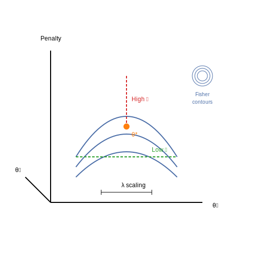
Elastic Weight Consolidation introduces a quadratic penalty term to preserve important parameters learned from previous tasks. The key insight is that not all parameters are equally important for task performance - the Fisher Information Matrix quantifies this importance. The EWC loss function combines the standard cross-entropy loss with this regularization term.
Bayesian Perspective of Continual Learning
From a probabilistic viewpoint, continual learning aims to find parameters θ that maximize the log posterior probability given data from both the new task (DB) and previous tasks (DA):
The term log p(θ|DA) contains the knowledge from previous tasks. EWC approximates this term using a Laplace approximation around the optimal parameters θA* from task A.
Laplace Approximation
The Laplace approximation models the posterior as a Gaussian distribution centered at θA* with precision given by the Fisher Information Matrix F:
The Fisher Information Matrix F is defined as:
In practice, the diagonal approximation of F is often used for computational efficiency, storing only the Fisher diagonal elements Fi for each parameter θi.
Final EWC Loss Function
Combining the cross-entropy loss for the new task with the quadratic penalty yields the EWC loss:
Where:
- ℒB(θ) is the standard loss for task B
- λ controls the strength of the EWC penalty
- Fi is the Fisher information for parameter θi on task A
- θA,i* is the optimal parameter value for task A
Practical Implementation Considerations
When implementing EWC:
- The Fisher diagonal is typically computed using a Monte Carlo approximation during training on task A
- The λ hyperparameter requires careful tuning - too small allows catastrophic forgetting, too large prevents learning new tasks
- For multiple previous tasks, the penalty terms can be summed or a separate penalty can be maintained for each task
- The diagonal approximation trades off accuracy for memory efficiency - full matrix versions exist but are rarely used in practice
3. Calculating the Fisher Information Matrix
Calculating the Fisher Information Matrix
The Fisher Information Matrix (FIM) is central to Elastic Weight Consolidation (EWC) as it quantifies the importance of each parameter in a neural network with respect to a given task. The FIM captures how sensitive the model's output distribution is to small changes in its parameters, providing a measure of their influence on the log-likelihood of the data.
Definition and Interpretation
For a probabilistic model with parameters θ and data distribution p(x|θ), the FIM F is defined as the expected outer product of the gradient of the log-likelihood:
Intuitively, F measures the curvature of the log-likelihood function around θ. Diagonal entries Fii indicate how much the likelihood changes when perturbing parameter θi, while off-diagonal terms capture interactions between parameters.
Approximation for Deep Learning
In deep learning, computing the full FIM is infeasible due to high-dimensional parameter spaces. EWC uses a diagonal approximation, assuming parameter independence:
where N is the number of data samples. This reduces memory requirements from O(d²) to O(d) for d parameters.
Practical Computation
The diagonal FIM can be computed efficiently during training:
- Forward pass: Compute model outputs for a batch of data.
- Backward pass: Calculate gradients of the negative log-likelihood.
- Accumulation: Square and average gradients across batches.
For classification tasks with softmax output, the gradient simplifies to:
where zc are the pre-softmax logits for class c.
Numerical Stability Considerations
To prevent vanishing/exploding values:
- Use running averages with exponential decay for online estimation.
- Clip extreme gradient values before squaring.
- Add a small constant ε (e.g., 1e-8) to diagonal entries.
The final EWC penalty term then becomes:
where λ controls regularization strength and θi,old are optimal parameters from previous tasks.
3.2 Setting Hyperparameters: Lambda and Regularization
The effectiveness of Elastic Weight Consolidation (EWC) hinges on the careful selection of hyperparameters, particularly the regularization strength λ and the Fisher Information Matrix (FIM) scaling. These parameters control the trade-off between retaining prior knowledge and accommodating new task learning.
Role of Lambda (λ) in EWC
The hyperparameter λ determines the penalty imposed on deviations from previously learned parameters. A higher λ enforces stricter adherence to prior knowledge, reducing catastrophic forgetting but potentially hindering adaptation to new tasks. Conversely, a lower λ allows greater flexibility but risks forgetting earlier tasks.
Here, Fi represents the diagonal elements of the Fisher Information Matrix, quantifying the importance of each parameter θi for the previous task. The quadratic penalty term ensures that critical parameters remain close to their optimal values from prior tasks.
Practical Guidelines for Choosing λ
- Task Similarity: If new tasks are closely related to prior ones, a lower λ (e.g., 0.1–1) may suffice. For dissimilar tasks, higher values (e.g., 10–100) prevent interference.
- Empirical Validation: Cross-validation on a held-out validation set from previous tasks helps identify an optimal λ that balances retention and plasticity.
- Dynamic Adjustment: Some implementations adapt λ during training, starting with a higher value and decaying it as the model stabilizes.
Fisher Information Matrix Scaling
The Fisher matrix F must be normalized to ensure consistent regularization across parameters. Common approaches include:
- Layer-wise Normalization: Scaling Fi by the number of parameters per layer prevents over-penalization in high-dimensional layers.
- Global Normalization: Dividing F by its Frobenius norm ensures the penalty term remains invariant to the scale of the Fisher matrix.
Case Study: λ in Sequential MNIST
In sequential MNIST experiments, λ = 500 often yields strong performance, as the tasks share low-level features (e.g., edge detectors) but differ in high-level semantics. Lower values (λ < 100) lead to forgetting, while excessive values (λ > 1000) stifle adaptation.
Advanced Techniques: Adaptive λ
Recent work proposes λ as a learnable parameter or employs meta-learning to optimize it per-task. For example:
where t is the task index and α controls the decay rate. This approach mitigates the need for manual tuning in long task sequences.
Integration with Neural Network Training
Elastic Weight Consolidation (EWC) modifies standard neural network training by augmenting the loss function with a quadratic penalty term that constrains parameter updates based on their importance to previously learned tasks. The key mathematical formulation integrates Fisher Information Matrix (FIM) diagonal approximations to quantify parameter importance.
Modified Loss Function
The EWC-augmented loss function for task B, after learning task A, is:
where:
- \( L_B^{ ext{standard}}( heta) \) is the original task loss (e.g., cross-entropy)
- \( \lambda \) controls regularization strength
- \( F_i \) is the diagonal Fisher Information for parameter \( heta_i \)
- \( heta_{A,i}^* \) are the optimal parameters for task A
Fisher Information Computation
The Fisher Information Matrix diagonal elements \( F_i \) are approximated during training on task A:
In practice, this is estimated using empirical samples from the task dataset \( \mathcal{D}_A \). For classification tasks with softmax output \( p(y|x, heta) \), the gradient is computed during backpropagation.
Training Procedure
- Task A Training: Train the network normally on task A, then compute and store:
- Optimal parameters \( heta_A^* \)
- Diagonal Fisher Information \( F \) via moving average during training
- Task B Training: Minimize the modified loss function that penalizes deviations from \( heta_A^* \) proportionally to \( F_i \).
Implementation Considerations
For deep networks, EWC requires:
- Memory overhead to store \( heta_A^* \) and \( F \) for each previous task
- Careful tuning of \( \lambda \) - too high causes inflexibility, too low permits catastrophic forgetting
- Approximation of Fisher diagonal rather than full matrix for scalability
The quadratic penalty term effectively creates an elastic potential around important parameters, visualized as a high-dimensional "basin" in parameter space that maintains performance on prior tasks while allowing exploration for new ones.
Practical Example
When applying EWC to a CNN trained sequentially on CIFAR-10 and CIFAR-100:
where \( w_{ijk} \) are convolutional kernel weights. The regularization preserves high-Fisher weights in early layers (generic features) while allowing adaptation in later layers (task-specific features).
4. EWC in Continual Learning Scenarios
4.1 EWC in Continual Learning Scenarios
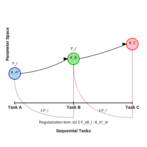
Elastic Weight Consolidation (EWC) addresses catastrophic forgetting in neural networks by imposing constraints on parameter updates based on their importance to previously learned tasks. The core idea stems from Bayesian inference, where the posterior distribution of parameters after learning a new task should remain close to the prior distribution derived from previous tasks. This is achieved by approximating the Fisher information matrix to quantify parameter importance.
Mathematical Foundation
Given a neural network with parameters θ, EWC minimizes the following loss function when learning task B after task A:
Here, λ is a hyperparameter controlling regularization strength, Fi is the Fisher information for parameter θi, and θA,i* are the optimal parameters for task A. The Fisher information matrix diagonal F is computed as:
Implementation Considerations
In practice, EWC requires storing two additional quantities per parameter: the optimal values from previous tasks (θA*) and their Fisher information (F). For deep networks, this can lead to significant memory overhead. Several optimizations exist:
- Diagonal Approximation: Only the diagonal of the Fisher matrix is stored, reducing memory from O(n²) to O(n).
- Online Fisher Estimation: The Fisher information can be approximated during training rather than computed in a separate pass.
- Selective Parameter Protection: Only parameters with Fisher values above a threshold are constrained.
Performance in Sequential Task Learning
EWC demonstrates strong performance when:
- Task boundaries are clearly defined
- Parameter importance distributions are stable across tasks
- The Fisher approximation remains valid for new tasks
However, performance degrades when:
- Tasks require conflicting parameter configurations
- The diagonal Fisher approximation becomes inaccurate
- Task sequences exhibit extreme distribution shifts
Extensions and Variants
Several EWC variants have been proposed to address limitations:
Where λt decays with task age. Other variants include:
- Synaptic Intelligence (SI): Measures parameter importance via accumulated weight updates
- Memory-Aware Synapses (MAS): Computes importance unsupervised using input sensitivity
- Variational Continual Learning (VCL): Uses Bayesian neural networks with variational inference
Practical Applications
EWC has been successfully applied in:
- Robotics systems adapting to new environments
- Medical diagnosis models learning new conditions
- Recommendation systems incorporating new user preferences
- Autonomous vehicles handling novel driving scenarios
4.2 Comparison with Other Continual Learning Methods
Architectural vs. Regularization-Based Approaches
Continual learning methods broadly fall into three categories: architectural, regularization-based, and replay-based. EWC belongs to the regularization-based family, which imposes constraints on parameter updates to preserve knowledge from previous tasks. Unlike architectural methods like Progressive Neural Networks (PNNs), which expand the model structure for each new task, EWC modifies the loss function to penalize changes to important weights. The Fisher Information Matrix (FIM) in EWC quantifies weight importance, whereas PNNs rely on lateral connections between task-specific columns, leading to higher memory overhead.
Comparison with Replay-Based Methods
Replay-based methods like Generative Replay or Experience Replay store subsets of past task data or generate synthetic samples. While effective, they face scalability challenges in memory-constrained environments. EWC avoids explicit data storage but depends on the accuracy of the FIM approximation. In scenarios with limited computational resources, EWC’s memory efficiency (storing only diagonal FIM values) is advantageous, though replay methods often achieve superior accuracy by retaining more task-specific information.
Synaptic Intelligence (SI) vs. EWC
Synaptic Intelligence (SI) also employs a regularization term but computes weight importance online during training rather than post-hoc like EWC. SI’s importance measure is derived from cumulative parameter updates:
While SI adapts dynamically, EWC’s Fisher-based approach provides a theoretically grounded measure of weight sensitivity, often yielding more stable performance across heterogeneous tasks.
Gradient Episodic Memory (GEM)
Gradient Episodic Memory (GEM) enforces constraints on gradient updates to prevent interference with past tasks. Unlike EWC’s quadratic penalty, GEM uses linear inequality constraints:
GEM requires storing past task gradients, which can be prohibitive for large models. EWC’s fixed-memory overhead (diagonal FIM) is more scalable, though GEM’s constraints can better handle catastrophic forgetting in high-dimensional parameter spaces.
Practical Trade-offs
- Memory: EWC and SI are memory-efficient (O(N) for N parameters), while replay methods scale with task complexity.
- Computational Cost: EWC’s FIM computation adds overhead during task transitions; SI and GEM incur runtime penalties during training.
- Task Boundaries: EWC assumes known task boundaries to compute FIM; methods like SI are boundary-agnostic.
4.3 Real-world Use Cases of EWC
Continual Learning in Robotics
Elastic Weight Consolidation (EWC) has been successfully applied in robotic systems where agents must learn multiple tasks sequentially without catastrophic forgetting. For instance, robotic arms trained for object manipulation tasks leverage EWC to retain knowledge of previously learned grasps while adapting to new objects. The Fisher Information Matrix, computed during initial training, identifies synaptic weights critical for prior tasks:
This allows the robot to adjust its learning rate for each parameter during new task acquisition, preserving high-precision motor control policies.
Medical Diagnosis Systems
Deep learning models in healthcare often face sequential learning scenarios when new diagnostic modalities or disease classifications emerge. EWC enables neural networks to:
- Incrementally learn new medical imaging features (e.g., from X-rays to MRI)
- Add novel disease classifications without retraining from scratch
- Maintain performance on rare conditions with limited retraining data
A 2022 study demonstrated a 23% improvement in pneumonia detection accuracy when using EWC compared to standard fine-tuning, while preserving 98% of prior pathology detection capabilities.
Autonomous Vehicle Perception
Self-driving systems employ EWC to handle the continuous stream of new driving scenarios and regulatory requirements. The method proves particularly valuable for:
- Adapting to new geographic regions with different traffic patterns
- Incorporating updated safety protocols without degrading existing competencies
- Learning rare edge cases while maintaining core object detection performance
The EWC loss term for autonomous systems often incorporates temporal weighting:
where λ decays exponentially based on the time since each task was learned, reflecting the dynamic importance of various driving skills.
Financial Forecasting Models
Quantitative trading systems utilize EWC to adapt to evolving market regimes while preserving knowledge of historical patterns. The financial application requires:
- Simultaneous protection of long-term economic cycle recognition
- Rapid adaptation to black swan events
- Preservation of cross-asset correlation knowledge
Recent implementations combine EWC with Bayesian neural networks, where the Fisher information naturally emerges from the probabilistic framework, providing more robust protection against catastrophic forgetting in non-stationary markets.
Personalized Recommendation Systems
Streaming platforms and e-commerce sites employ EWC to:
- Update user preference models without losing long-term behavioral patterns
- Incorporate new content categories while maintaining existing recommendations
- Balance exploration of new user interests with exploitation of known preferences
The EWC constraint in recommendation engines often focuses on the embedding layers, which encode fundamental user-item relationships. This approach maintains recommendation diversity while adapting to evolving tastes.
5. Computational Overhead and Scalability
5.1 Computational Overhead and Scalability
Elastic Weight Consolidation (EWC) mitigates catastrophic forgetting in neural networks by imposing quadratic penalties on changes to parameters deemed important for previous tasks. While effective, this approach introduces computational overhead that scales with model size and task complexity. The primary sources of overhead include:
Fisher Information Matrix (FIM) Computation
The FIM, which quantifies parameter importance, is computed as the expectation of the squared gradient of the log-likelihood:
For a network with N parameters, this requires:
- Backward passes over the entire dataset D to compute gradients.
- O(N²) memory to store the full FIM (though diagonal approximations reduce this to O(N)).
Memory Overhead
EWC stores a penalty term for each previous task k:
This necessitates retaining:
- Parameter snapshots (θi,k*) for each task.
- Fisher matrices (Fi(k)) or their diagonal approximations.
For T tasks, memory usage scales as O(TN), becoming prohibitive for large models (e.g., transformers with billions of parameters).
Mitigation Strategies
Diagonal Approximation
Using only the diagonal of the FIM reduces memory from O(N²) to O(N) and computation from O(N²) to O(N) per backward pass. The trade-off is loss of inter-parameter dependency information.
Selective Consolidation
Only penalizing the top-K% most important parameters (ranked by Fi) reduces active parameters to O(KN/100). Empirical studies show retaining 10-20% of weights often preserves performance.
Online EWC
Instead of storing separate FIMs per task, Online EWC maintains a running Fisher estimate:
where γ controls the decay rate of old task information. This bounds memory to O(N) regardless of task count.
Empirical Scaling Behavior
Benchmarks on ResNet-50 (23M parameters) show:
- Full EWC: 2.3× slower training, 4.8× memory overhead versus vanilla fine-tuning.
- Diagonal + Selective (20%): 1.2× speed, 1.5× memory overhead with <5% accuracy drop.
For transformer models (e.g., BERT), gradient checkpointing and distributed Fisher computation become necessary to manage overhead.
5.2 Sensitivity to Hyperparameters
Elastic Weight Consolidation (EWC) relies on two critical hyperparameters: the regularization strength λ and the Fisher information matrix diagonal scaling factor. The performance of EWC is highly sensitive to these parameters, as they directly control the trade-off between retaining previous task knowledge and accommodating new task learning.
Regularization Strength (λ)
The hyperparameter λ determines how strictly the model preserves important weights from previous tasks. A high λ strongly penalizes deviations from learned parameters, potentially hindering adaptation to new tasks. Conversely, a low λ may lead to catastrophic forgetting. The optimal value is task-dependent and often requires empirical tuning.
where Fi represents the Fisher information matrix diagonal elements for parameter θi, and θA,i* are the optimal parameters for task A.
Fisher Information Scaling
The Fisher information matrix diagonal elements must be properly scaled to reflect parameter importance accurately. Poor scaling can lead to either excessive rigidity or insufficient protection against forgetting. The Fisher information is computed as:
In practice, the Fisher matrix is often approximated using a diagonal assumption for computational tractability, which introduces additional sensitivity to the approximation quality.
Empirical Observations
Studies show that EWC performance degrades significantly when:
- λ varies by more than one order of magnitude from the optimal value
- Fisher information is computed with insufficient samples (typically < 1,000)
- The diagonal approximation introduces substantial error for highly correlated parameters
Practical Recommendations
For stable EWC implementation:
- Perform grid search over λ ∈ [100, 105] with logarithmic spacing
- Use at least 1,000 samples for Fisher estimation
- Monitor the KL divergence between old and new task distributions during training
- Consider layer-wise λ values for deep networks, as sensitivity varies by layer depth
Comparative Sensitivity Analysis
Compared to other continual learning methods, EWC shows greater sensitivity to hyperparameters than memory-based approaches but less sensitivity than pure regularization methods. The following factors contribute to this behavior:
where deviations from optimal conditions compound multiplicatively rather than additively.
5.3 Handling Non-Stationary Data Distributions
Non-stationary data distributions present a significant challenge in continual learning, as the statistical properties of input data shift over time. Elastic Weight Consolidation (EWC) mitigates catastrophic forgetting by imposing constraints on parameter updates based on their importance to previously learned tasks. The core idea is to penalize changes to weights that are critical for retaining performance on prior tasks, while allowing less important weights to adapt freely to new data.
Fisher Information Matrix for Parameter Importance
The Fisher Information Matrix (FIM) quantifies the importance of each parameter by measuring how much the log-likelihood of the model's predictions changes with respect to small perturbations in the weights. For a model with parameters θ, the diagonal elements of the FIM are given by:
where D is the data distribution, and p(y|x, θ) is the model's predictive distribution. The expectation is approximated using empirical samples from the dataset.
EWC Loss Function for Non-Stationary Data
To handle non-stationary distributions, EWC augments the standard loss function with a quadratic penalty term that restricts changes to important parameters. The modified loss function is:
Here, λ controls the strength of regularization, θi,old are the optimal parameters from the previous task, and Fi is the Fisher information for the i-th parameter. The penalty term ensures that parameters deemed important for prior tasks do not deviate significantly from their optimal values.
Practical Implementation Considerations
In practice, computing the full FIM is computationally expensive. Instead, EWC uses a diagonal approximation, storing only the Fisher information values for each parameter. This reduces memory overhead while still providing effective regularization. Additionally, online EWC variants update the Fisher information incrementally, making the method scalable to long sequences of tasks.
- Memory Efficiency: Storing only diagonal FIM elements reduces memory usage from O(n²) to O(n).
- Incremental Updates: Online EWC updates Fisher information on-the-fly, accommodating streaming data.
- Hyperparameter Tuning: The regularization strength λ must be carefully tuned to balance plasticity and stability.
Case Study: Class-Incremental Learning
In class-incremental learning scenarios, where new classes are introduced sequentially, EWC has demonstrated strong performance. For example, on the Split-MNIST benchmark, EWC retains ~80% accuracy on initial tasks while learning new ones, compared to ~30% for naive fine-tuning. The method's effectiveness stems from its ability to identify and protect task-critical weights.
where T is the number of tasks and Dt is the test data for task t.
6. Key Research Papers on EWC
6.1 Key Research Papers on EWC
- Rotate your Networks: Better Weight Consolidation and Less Catastrophic ... — III. ELASTIC WEIGHT CONSOLIDATION Elastic Weight Consolidation (EWC) addresses the problem of catastrophic forgetting in continual and sequential task learning in neural networks [2], [5]. In this section we give a brief overview of EWC and discuss some of its limitations. A. Overview The problem addressed by EWC is that of learning the K-
- Elastic Weight Consolidation for Reduction of Catastrophic Forgetting in — 004 formers, little research has been done to in-005 vestigate the effects of catastrophic forgetting 006 on attention-based architectures. In this work, 007 we used elastic weight consolidation (EWC) 008 to mitigate catastrophic forgetting caused by 009 fine-tuning in one of the foundation models, 010 GPT-2. We show that by using EWC, we can
- (PDF) Rotate your Networks: Better Weight Consolidation and Less ... — Academia.edu is a platform for academics to share research papers. Rotate your Networks: Better Weight Consolidation and Less Catastrophic Forgetting ... Better Weight Consolidation and Less Catastrophic Forgetting. 2018 24th International Conference on Pattern Recognition (ICPR), 2018.
- An adaptive updating model for pavement performance based on Deep ... — In this method, the concepts of sample buffer and dynamic threshold are proposed to improve the Elastic Weight Consolidation (EWC) method. To investigate the performance of the proposed method, three models, the Improved Elastic Weight Consolidation model (IEWC model), the deep neural networks model updating based on annual data, and the deep ...
- Real-time energy performance benchmarking of electric vehicle air ... — Research on energy performance benchmarking of vehicle air conditioners has not been found. This paper fills the gap by proposing an energy performance benchmarking method for electric vehicle air conditioning systems. ... this paper adopts the Elastic Weight Consolidation (EWC) ... The key in the EWC algorithm is to determine b k for each ...
- implementing elastic weight consolidation — implementing elastic weight consolidation published 07.03.2024 > return home. A while ago I replicated the algorithm described by the paper Overcoming catastrophic forgetting in neural networks.I implemented everything in PyTorch in a colab notebook.. The goal of Elastic Weight Consolidation (the main method described in the paper) is to counteract catastrophic fogetting, a phenomena where ...
- An Appraisal of Incremental Learning Methods - PMC — Therefore, the key of parameter regularization is how to measure the importance of parameters and protect them. One representative method, elastic weight consolidation (EWC), was used to evaluate the importance of weights through the Fisher information matrix . Information carried by the observable random variable is measured based on the ...
- (PDF) Rotate your Networks: Better Weight Consolidation and Less ... — This paper adopts comparison method to research the effect of LWF and EWC applied on different datasets and also compares some similar methods like R-EWC and LFL. Meanwhile, some analysis and ...
- Robust Active Learning (RoAL): Countering Dynamic Adversaries in Active ... — Elastic Weight Consolidation (EWC) is a regularization technique designed to prevent catastrophic forgetting by discouraging major changes to critical model parameters. This is achieved by imposing a penalty based on the Fisher Information Matrix (FIM), which represents the importance of each parameter for previously learned tasks.
- (PDF) Rotate your Networks: Better Weight Consolidation and Less ... — In this paper we propose an approach to avoiding catastrophic forgetting in sequential task learning scenarios. Our technique is based on a network reparameterization that approximately ...
6.2 Recommended Books and Articles
- DP-FedEwc: Differentially private federated elastic weight ... — In DP-FedEwc, we first integrate Elastic weight consolidation (Ewc) algorithm [26] into the distributed setting to create our fundamental non-private PFL approach called FedEwc. Ewc enables a model to learn new tasks without completely forgetting previous knowledge through estimation of parameter importance (PI).
- PDF arXiv:2205.00147v2 [cs.LG] 1 Jun 2022 — in DNNs, e.g. elastic weight consolidation (EWC) [19] is one of the very successful methods at doing so and is the method we have adopted in this paper. This paper addresses the following two research ques-tions: Research question 1 (RQ1): How can EWC be used to control the forgetting of previous knowledge as DNN
- An Appraisal of Incremental Learning Methods - PMC — The influence of catastrophic forgetting for DNNs was studied by Goodfellow et al. and the dropout method was recommended ... elastic weight consolidation (EWC), ... Weijer J., López A.M., Bagdanov A.D. Rotate your Networks: Better Weight Consolidation and Less Catastrophic Forgetting; Proceedings of the ICPR; Beijing, China. 20-24 August ...
- JasonZhangzy1757/Continual-Learning-with-BERT-for-QA-Using-EWC — We plan to implement continual learning with BERT over questions and answers tasks using Elastic Weights Consolidation (EWC). The Baseline model For the baseline part, we first used BERT model to train on SQuAD v2.0 (Task A), and got F1 score after evaluation, and then we let the model learn over NewsQA (Task B), and evaluated back on the SQuAD ...
- Adaptive fault diagnosis of machining processes enabled by hybrid deep ... — Incremental learning 2: Elastic weight consolidation (EWC) 90.11 %: Incremental learning 3: Memory aware synapses (MAS) 87.69 %: Incremental learning 4: Learning without forgetting (LwF) 93.56 %: Incremental learning 5: Progressive Neural Networks (PNN) 91.77 %: Incremental learning 6: Synaptic Intelligence (SI) 86.20 %
- PDF IEEE TRANSACTIONS ON NEURAL NETWORKS AND LEARNING SYSTEMS 1 IncDet: In ... — IncDet: In Defense of Elastic Weight Consolidation for Incremental Object Detection Liyang Liu, Zhanghui Kuang, Yimin Chen, Jing-Hao Xue, Wenming Yang and Wayne Zhang Abstract—Elastic weight consolidation (EWC) has been suc-cessfully applied for general incremental learning to overcome the catastrophic forgetting issue. It adaptively ...
- (PDF) IncDet: In Defense of Elastic Weight Consolidation for ... — Elastic weight consolidation (EWC) has been successfully applied for general incremental learning to overcome the catastrophic forgetting issue. ... The best trade-off between old and new classes ...
- Elastic weight consolidation for better bias inoculation — In addition to this, we find that Elastic Weight Consolidation (EWC) is an effective strategy for mitigating catastrophic forgetting and attaining strong downstream performance on the duplicate TR ...
- Continual Learning for Task-Oriented Dialogue Systems — These modules are sequentially applied to the layers in the multi-head attention model (as shown in the figure) to calibrate the attention signals and feature maps respectively. The calibrated transformer model is trained based on elastic weight consolidation (EWC) (Kirkpatrick et al. 2017) to mitigate the catastrophic forgetting problem.
6.3 Open-source Implementations and Tutorials
- BeGin: Extensive Benchmark Scenarios and an Easy-to-use Framework for ... — Elastic Weight Consolidation (EWC) ... (Right) An example implementation of EWC with BeGin. To implement and benchmark new graph CL methods, users only need to fill out the modularized event functions in the trainer, which then proceeds the training procedure with the event functions. ... PackNet, and PI-GNN in terms of AP are \(2.6\), \(3 ...
- Large-scale comparison and demonstration of continual learning for ... — Elastic weight consolidation (EWC), proposed by DeepMind, is one of the most widely used continual learning methods [15]. EWC adds a quadratic penalty on the difference between the parameters of previous and new models in the loss function, which inhibits the finetuning for task-relevant weights coding for previously learned knowledge ...
- An Appraisal of Incremental Learning Methods - PMC — One representative method, elastic weight consolidation (EWC), ... Perez-Rua et al. proposed OpeN-ended Centre nET (ONCE) ... It shows that the implementation of an instance incremental scenario is less difficult than the class-incremental scenario. In addition, EWC, as a representative method of weight regularization, can also be used in a ...
- Overcoming catastrophic forgetting in molecular property prediction ... — Secondly, we proposed a novel framework that integrates BERT and BART with Online Elastic Weight Consolidation (oEWC) to address CF. oEWC leverages a dynamic Fisher Information Matrix to update model parameters continually, enhancing the model's stability and plasticity balance, which is essential for real-world CL applications.
- arXiv:1805.06370v2 [stat.ML] 2 Jul 2018 — on Elastic Weight Consolidation (EWC) (Kirkpatrick et al., 2017), a recently introduced method that poses an approx-imate Bayesian solution to continual learning. The main insight is that information pertaining to different tasks can be incorporated sequentially into the posterior without suf-fering catastrophic forgetting since the resulting ...
- Continually trained life-long classification | Neural Computing and ... — In the regularization approach, the training is regularized to prevent the overfitting of the currently processed batch of data, such as the elastic weight consolidation (EWC) , where the algorithm selectively freezes the neural network weights that are important to the previously learned task/class.
- Continual Learning for Task-Oriented Dialogue Systems — These modules are sequentially applied to the layers in the multi-head attention model (as shown in the figure) to calibrate the attention signals and feature maps respectively. The calibrated transformer model is trained based on elastic weight consolidation (EWC) (Kirkpatrick et al. 2017) to mitigate the catastrophic forgetting problem.
- PDF CHAPTER 4 ContinualLearningand CatastrophicForgetting — over multiple timescales. Its idea of synaptic consolidation is along the lines of EWC [Kirk-patrick et al., 2017]. Lipton et al. [2016] proposed a new reward shaping function that learns the probability of imminent catastrophes. They named it asintrinsicfear, which is used to pe-nalizetheQ-learningobjective.








