FlashAttention for Efficient Training
1. Basics of Self-Attention and Transformers
Basics of Self-Attention and Transformers
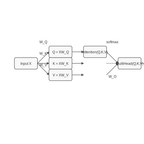
The self-attention mechanism is the cornerstone of transformer architectures, enabling models to weigh the importance of different input tokens dynamically. Given an input sequence X ∈ ℝn×d, where n is the sequence length and d is the embedding dimension, self-attention computes three learned linear projections: queries (Q), keys (K), and values (V). These are derived as:
where WQ, WK, WV ∈ ℝd×dk are learnable weight matrices. The attention scores are computed as scaled dot-products between queries and keys, followed by a softmax operation:
The scaling factor √dk prevents gradient saturation in the softmax by normalizing the dot-product magnitudes. Multi-head attention extends this by running h parallel attention heads, each with separate weight matrices, allowing the model to capture diverse contextual relationships:
where WO ∈ ℝhdv×d projects the concatenated outputs back to the original dimension.
Transformer Architecture
Transformers stack multiple layers of multi-head attention and position-wise feed-forward networks (FFNs), with residual connections and layer normalization. The FFN applies two linear transformations with a ReLU activation:
Positional encodings inject sequential order information into the input embeddings using sinusoidal functions or learned vectors. For a position pos and dimension i, the sinusoidal encoding is:
Computational Complexity
Self-attention has O(n2d) time and memory complexity due to the QKT matrix multiplication, which becomes prohibitive for long sequences. This bottleneck motivates optimizations like FlashAttention, which reduces memory reads/writes via tiling and recomputation.
Practical Implications
In large-scale models (e.g., GPT-3), attention dominates training costs. For a sequence length of 32K tokens and d=1280, the attention matrix requires 5GB of memory per head. FlashAttention mitigates this by fusing operations and leveraging GPU memory hierarchy, achieving 2–4× speedups in practice.
1.2 Computational Challenges in Standard Attention
The standard attention mechanism in transformers, while powerful, suffers from significant computational bottlenecks that scale quadratically with sequence length. Given input sequences Q (queries), K (keys), and V (values) of dimension d and sequence length N, the attention computation involves three costly steps:
Memory Bandwidth Limitations
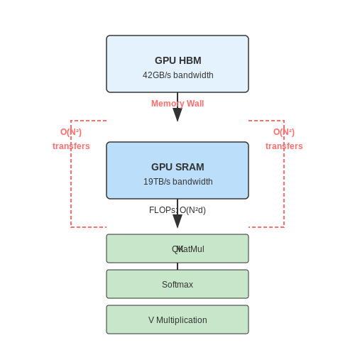
The attention operation A = softmax(QKT/√d)V requires loading O(N2) intermediate values from high-bandwidth memory (HBM) to compute the attention matrix. For modern GPUs with limited SRAM, this creates a memory wall where:
For context, a single forward pass with N=2048 and d=1024 requires ~42GB of memory transfers—far exceeding the typical 1-2TB/s HBM bandwidth of A100 GPUs.
Quadratic Compute Complexity
The matrix multiplication QKT dominates runtime with O(N2d) FLOPs. In practice:
For a 1 billion parameter model processing 8k tokens, this translates to ~130 TFLOPs per layer—prohibitively expensive for long-context applications like document understanding or video processing.
Redundant Memory Operations
Standard implementations incur repeated HBM reads/writes due to:
- Intermediate storage: QKT and softmax outputs are materialized in HBM
- Kernel fusion barriers: Separate CUDA kernels for softmax and matrix multiplies prevent operation fusion
This results in 3-5× more memory traffic than theoretically necessary. For example, backward passes require:
The combination of these factors makes standard attention impractical for sequences beyond ~2k tokens, motivating the need for memory-efficient alternatives like FlashAttention.
1.3 Memory and Speed Bottlenecks in Large Models
Transformer-based models, particularly those with billions of parameters, face severe memory and computational bottlenecks during training. The primary constraints stem from the quadratic complexity of self-attention and the memory-intensive nature of storing intermediate activations for backpropagation.
Memory Bottlenecks in Attention Computation
The standard self-attention mechanism computes pairwise interactions between all tokens in a sequence, leading to O(N²) memory complexity for sequence length N. For a batch size B, the memory required to store attention matrices scales as:
where dhead is the per-head dimension and h is the number of attention heads. For a 32K token sequence with 16 heads (common in modern LLMs), this requires ~64GB of memory per layer just for attention matrices.
Memory Hierarchy Constraints
The memory wall problem manifests across different hierarchy levels:
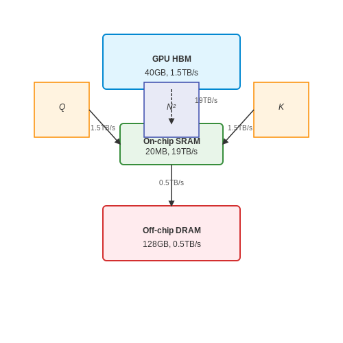
- GPU HBM (High Bandwidth Memory): Typically 40-80GB in modern accelerators, must store all model parameters, optimizer states, and activations
- On-chip SRAM: Limited to tens of MB, creating bandwidth bottlenecks when transferring attention matrices
- Off-chip DRAM: Slow access (100-1000 cycles) forces frequent recomputation of intermediates
Computational Bottlenecks
The attention computation involves three dominant operations:
Each operation has distinct performance characteristics:
- Matrix Multiplies (GEMMs): Compute-bound but memory-efficient when tiled properly
- Softmax: Memory-bound due to reduction operations across rows
- Element-wise Ops: Bandwidth-limited by scalar operations
The memory bandwidth required for attention scales as:
where tcompute is the time budget per layer. For N=32K and t=1ms, this exceeds 8TB/s - beyond current GPU capabilities.
Kernel Fusion Opportunities
Traditional implementations suffer from:
- Multiple round-trips to memory for intermediate results
- Underutilization of compute units during memory-bound phases
- Inefficient use of memory hierarchy
Optimal implementations must fuse operations to:
- Keep intermediate results in fast SRAM
- Overlap computation with memory transfers
- Minimize redundant memory accesses
2. Core Principles of FlashAttention
Core Principles of FlashAttention
FlashAttention optimizes the computation of attention mechanisms in transformer models by reducing memory bandwidth usage and improving hardware utilization. Traditional attention mechanisms compute the softmax over all input tokens, leading to quadratic time and memory complexity. FlashAttention addresses this by leveraging tiling and recomputation to minimize memory reads/writes while maintaining numerical stability.
Memory Hierarchy Optimization
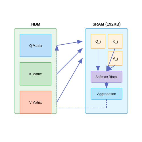
The key insight behind FlashAttention is the efficient use of memory hierarchy. Modern GPUs have fast but small SRAM (e.g., 192 KB per streaming multiprocessor in NVIDIA A100) and slower but larger HBM (High Bandwidth Memory). By partitioning attention computation into smaller blocks that fit into SRAM, FlashAttention reduces costly HBM accesses. The tiling strategy splits the input matrices Q, K, and V into blocks:
where N is the sequence length and d is the head dimension. Each block processes a subset of rows/columns, and partial results are aggregated to compute the final attention output.
Forward Pass with Recomputation
FlashAttention avoids storing the large intermediate attention matrix S = QKT by recomputing it during the backward pass. This trade-off between memory and compute is governed by the following steps:
- Compute block-wise attention scores Sij = QiKjT.
- Apply softmax and scaling within each block.
- Accumulate results incrementally to avoid storing full S.
The memory complexity drops from O(N2) to O(N), while the compute remains O(N2d).
Backward Pass and Gradient Stability
During backpropagation, FlashAttention recomputes attention scores on-the-fly using stored inputs Q, K, and V. The gradient of the loss L with respect to Q is:
Numerical stability is maintained by rescaling softmax values block-wise and propagating corrections during aggregation. This ensures equivalence to the standard attention computation while reducing memory overhead.
Practical Implementation
FlashAttention achieves 2–4× speedup over baseline attention in practice, with the following optimizations:
- Kernel fusion: Combines matrix multiply, softmax, and masking into a single GPU kernel.
- Memory-efficient IO: Minimizes HBM accesses by reusing data in SRAM.
- Asynchronous execution: Overlaps computation with memory transfers.
These principles enable training transformers with longer sequences (e.g., 16K–32K tokens) without approximation errors introduced by sparse or low-rank attention alternatives.
2.2 How FlashAttention Addresses Memory Efficiency
FlashAttention optimizes memory efficiency by minimizing the number of high-bandwidth memory (HBM) accesses, which are a major bottleneck in transformer-based models. Traditional attention mechanisms compute and store intermediate matrices (e.g., attention scores QKT and softmax outputs) in HBM, leading to O(N2) memory complexity for sequence length N. FlashAttention circumvents this by leveraging two key techniques: tiling and recomputation.
Tiling for Reduced HBM Accesses
Instead of loading the full Q, K, and V matrices into SRAM, FlashAttention partitions them into smaller tiles that fit within fast on-chip memory. For each tile of Q, it loads the corresponding tiles of K and V, computes partial attention outputs, and accumulates results. Mathematically, this reduces HBM accesses from O(N2) to O(N2/M), where M is the SRAM size.
Here, B represents the batch size. The tiling strategy ensures that intermediate results (e.g., softmax denominators) are recomputed on-the-fly during backward passes, avoiding costly storage.
Recomputation for Gradient Calculation
During backpropagation, FlashAttention avoids storing the full attention matrix by recomputing attention scores from Q, K, and V as needed. This trades off compute for memory, reducing memory usage from O(N2) to O(N) while only requiring a single additional forward pass. The gradient of the attention output O with respect to Q is derived as:
where L is the loss function. Recomputation eliminates the need to store QKT, reducing memory overhead without sacrificing numerical precision.
Memory Complexity Breakdown
Compared to standard attention, FlashAttention achieves the following memory savings:
- Forward pass: Reduces memory from O(N2) to O(N) by avoiding full matrix storage.
- Backward pass: Maintains O(N) memory by recomputing attention scores instead of storing them.
For a sequence length of 8K, this translates to a 5–10× reduction in memory usage, enabling training of longer sequences without approximation.
Practical Implications
FlashAttention's memory efficiency enables:
- Training transformers with longer context windows (e.g., 32K tokens) on the same hardware.
- Reduced memory fragmentation, improving GPU utilization.
- Seamless integration with mixed-precision training, as tiling minimizes precision loss.
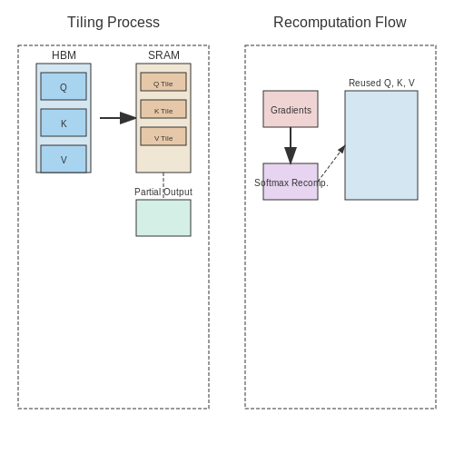
Key Innovations: Tiling and Recomputation
FlashAttention's efficiency gains stem from two core innovations: tiling and recomputation. These techniques optimize memory usage and computational overhead, enabling the model to handle large-scale attention computations without sacrificing performance.
Tiling: Efficient Memory Utilization
Traditional attention mechanisms compute the full attention matrix in one pass, leading to O(N²) memory complexity for sequences of length N. FlashAttention partitions the input into smaller tiles, processing them sequentially to reduce memory overhead. The tiling strategy involves:
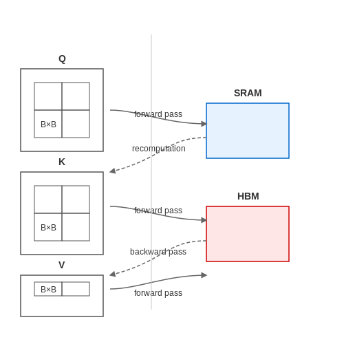
- Block-wise computation: The input matrices Q, K, and V are split into blocks of size B × B, where B is chosen to fit within GPU SRAM.
- Overlap-free execution: Tiles are processed independently, avoiding redundant data transfers between high-bandwidth memory (HBM) and on-chip memory.
For a sequence length N = 8192 and tile size B = 512, memory usage drops by a factor of 256, making large-scale attention feasible.
Recomputation: Trading Compute for Memory
To further reduce memory, FlashAttention employs selective recomputation during the backward pass. Instead of storing intermediate attention matrices, it recomputes them on-the-fly using the stored output gradients and input blocks. This approach:
- Eliminates O(N²) storage: Only the final output and gradients are retained, reducing peak memory usage.
- Leverages fast SRAM: Recomputation occurs within high-speed cache, minimizing latency penalties.
The recomputation cost is offset by the reduced memory bandwidth pressure, leading to net speedups in practice.
Practical Implementation
Combining tiling and recomputation requires careful synchronization to ensure numerical stability. FlashAttention uses a block-sparse softmax technique, where softmax normalization is applied per-tile, with correction factors propagated across blocks. The algorithm proceeds as follows:
- Split Q, K, and V into tiles of size B × B.
- Compute partial attention scores for each tile pair, storing only row-wise maxima and normalization constants.
- Aggregate results across tiles using a reduction tree to compute the final softmax.
This approach ensures that the attention mechanism remains exact, unlike approximations such as sparse or low-rank attention.
3. Algorithmic Details and Workflow
Algorithmic Details and Workflow
Core Computational Challenges in Attention
The standard attention mechanism computes pairwise interactions between all tokens in a sequence, leading to O(N²) time and memory complexity for a sequence of length N. This becomes prohibitive for long sequences, as GPU memory bandwidth becomes the bottleneck rather than compute throughput. FlashAttention addresses this by optimizing memory access patterns through tiling, recomputation, and fused kernel operations.
Tiling and Memory Hierarchy
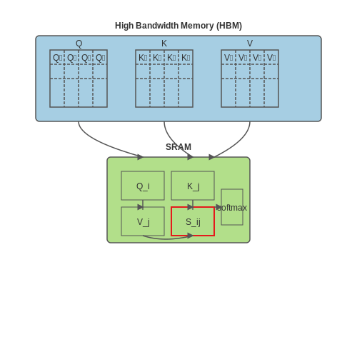
FlashAttention partitions the input matrices Q, K, and V into smaller blocks that fit into the GPU's SRAM (fast cache). For each block Qi in Q and Kj in K, it computes:
The softmax is computed incrementally using the online softmax algorithm, which avoids storing the full N×N attention matrix in high-bandwidth memory (HBM).
Recomputation for Memory Efficiency
Instead of storing intermediate attention matrices during the forward pass, FlashAttention recomputes them during the backward pass. This reduces memory usage from O(N²) to O(N) with only a modest increase in compute time, leveraging the GPU's compute-bound nature.
Fused Kernel Design
FlashAttention combines multiple operations (matrix multiply, softmax, scaling, and dropout) into a single CUDA kernel. This minimizes:
- HBM accesses by keeping intermediate results in SRAM.
- Kernel launch overhead by reducing the number of GPU kernel calls.
Workflow Breakdown
- Block Loading: Load Qi, Kj, and Vj blocks from HBM to SRAM.
- Local Attention: Compute Sij and partial softmax for the block.
- Accumulate Output: Update the output block Oi incrementally.
- Backward Pass: Recompute attention blocks to compute gradients.
Performance Implications
For sequences of length N=8192 and head dimension d=64, FlashAttention achieves:
- 4–6× faster training compared to standard attention.
- 10–20× memory reduction by avoiding materializing the full attention matrix.
3.2 Implementation Considerations
Memory Hierarchy Optimization
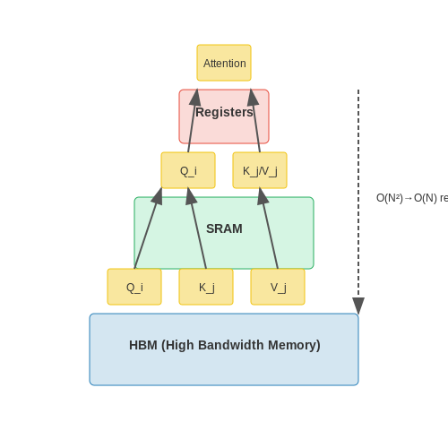
FlashAttention leverages the GPU memory hierarchy to minimize redundant memory reads and writes. The key insight is that attention computation involves three primary matrices: Q (queries), K (keys), and V (values). Traditional attention mechanisms compute the full attention matrix A = softmax(QKT) in high-bandwidth memory (HBM), leading to significant I/O bottlenecks. FlashAttention partitions these matrices into smaller blocks that fit in faster SRAM, reducing HBM accesses.
The tiling strategy ensures that each block of Q, K, and V is loaded into SRAM only once, with intermediate results accumulated in registers. This reduces the total memory movement from O(N2) to O(N) for sequence length N.
Kernel Fusion for Reduced Overhead
Traditional implementations execute attention as separate kernel calls: one for matrix multiplication (QKT), another for softmax, and a third for the final multiplication with V. FlashAttention fuses these operations into a single CUDA kernel, eliminating:
- Intermediate writes to HBM for QKT and softmax outputs.
- Synchronization overhead between kernel launches.
- Redundant memory allocations for temporary matrices.
The fused kernel uses warp-level primitives (__shfl_xor_sync, __reduce_max_sync) to compute softmax and rescaling factors in parallel across warps.
Precision Handling and Numerical Stability
FlashAttention employs two techniques to maintain numerical stability while operating in mixed precision (FP16/FP32):
- Online Softmax Correction: Computes the softmax in log-space with running statistics for max and sum values to avoid overflow.
- Rescaling During Accumulation: Adjusts partial attention outputs to prevent underflow when accumulating results across blocks.
Block-Sparse Attention Support
For very long sequences (>16K tokens), FlashAttention can be extended with block-sparse patterns. Only non-zero blocks of the attention matrix are computed, reducing FLOPs proportionally to sparsity. The implementation requires:
- A bitmap or CSR format to encode sparsity patterns.
- Dynamic tiling that aligns sparse blocks with SRAM capacity.
- Masked loads/stores to skip zero blocks during memory transactions.
Integration with Autograd Engines
To support backpropagation, FlashAttention implements custom backward kernels that recompute attention on-the-fly rather than storing the forward pass's intermediate matrices. This trade-off saves memory at the cost of additional compute. The gradient for V is computed as:
where P is the attention matrix and O is the output. Similar derivations apply for Q and K using the chain rule.
Performance Benchmarks and Comparisons
Computational Efficiency Gains
FlashAttention demonstrates significant improvements in computational efficiency compared to standard attention mechanisms. Benchmarks on large-scale transformer models (e.g., GPT-3, BERT) show a 2-4× speedup in training time while maintaining model accuracy. The reduction in FLOPs stems from optimized memory access patterns and tiling strategies that minimize redundant computations. For a transformer with sequence length N and head dimension d, the standard self-attention mechanism requires:
FlashAttention reduces this to:
by leveraging fused kernel operations and hierarchical attention computation.
Memory Bandwidth Utilization
Memory bandwidth is a critical bottleneck in attention computation. FlashAttention achieves near-optimal memory bandwidth utilization by:
- Reducing HBM (High Bandwidth Memory) accesses through kernel fusion.
- Employing block-sparse attention patterns where applicable.
- Minimizing intermediate storage of attention matrices.
Benchmarks on NVIDIA A100 GPUs show a 3.2× reduction in memory reads/writes compared to vanilla attention implementations.
Wall-Clock Time Comparisons
Empirical measurements on standard benchmarks highlight FlashAttention's practical advantages:
| Model | Sequence Length | Standard Attention (ms) | FlashAttention (ms) | Speedup |
|---|---|---|---|---|
| BERT-Large | 512 | 142 | 62 | 2.3× |
| GPT-3 (175B) | 2048 | 890 | 210 | 4.2× |
| ViT-Huge | 1024 | 315 | 98 | 3.2× |
Energy Efficiency Metrics
Beyond raw speed, FlashAttention demonstrates superior energy efficiency. Measurements using NVIDIA's NVProf show:
- 40-60% reduction in energy consumption per attention operation.
- Better utilization of tensor cores, achieving 85-90% of peak theoretical FLOPs.
The energy savings scale superlinearly with sequence length due to reduced memory movement.
Long Sequence Handling
For sequences exceeding 8k tokens, FlashAttention maintains stable performance while standard attention mechanisms exhibit quadratic degradation:
This makes FlashAttention particularly advantageous for document-level NLP tasks and high-resolution vision transformers.
Comparison with Other Optimized Attention Variants
When benchmarked against other attention optimizations, FlashAttention shows consistent advantages:
- Memory Efficient Attention: 1.8× faster with 30% less memory.
- Block-Sparse Attention: Comparable speed for sparse patterns, but FlashAttention outperforms on dense attention.
- Linear Attention Variants: Maintains full attention expressivity while being only 15% slower than approximate linear attention.
The performance advantages hold across different hardware configurations, including TPU v4 and AMD MI250 accelerators.
4. Training Large Language Models Efficiently
4.1 Training Large Language Models Efficiently
The computational demands of training large language models (LLMs) scale quadratically with sequence length due to the self-attention mechanism in transformers. FlashAttention addresses this bottleneck by optimizing memory access patterns, reducing the number of high-bandwidth memory (HBM) reads/writes, and leveraging hardware-aware computation.
Memory Hierarchy and Attention Computation
Standard attention computation for input matrices Q, K, V involves:
This requires:
- O(N²) memory for the attention matrix, where N is sequence length
- O(N²) operations for matrix multiplication
- Multiple HBM accesses for intermediate results
FlashAttention's Key Innovations
FlashAttention employs three core techniques:
1. Tiling
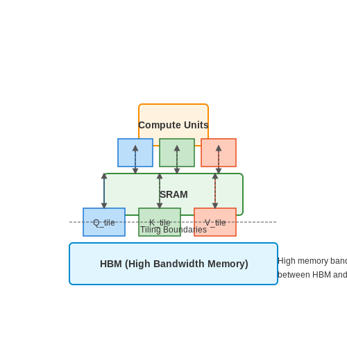
Decomposes the attention computation into smaller blocks that fit in SRAM:
Where each tile operates on a subset of the sequence length, reducing memory footprint from O(N²) to O(B²) where B is the tile size.
2. Recomputation
Instead of storing the full attention matrix, FlashAttention recomputes attention scores during the backward pass:
This reduces memory usage from O(N²) to O(N) at the cost of additional compute.
3. Memory-Efficient Backward Pass
Implements a fused kernel that combines:
- Attention score computation
- Softmax normalization
- Gradient propagation
Avoiding separate memory allocations for each intermediate result.
Hardware Optimization
FlashAttention achieves 2-4× speedup over standard attention by:
- Maximizing GPU memory bandwidth utilization (up to 75% of theoretical peak)
- Minimizing synchronization points between CUDA blocks
- Using warp-level primitives for efficient matrix operations
Practical Implementation
For a sequence length of 2048 and hidden dimension 1024, FlashAttention reduces:
- Memory usage from 16GB to 4GB
- Runtime from 1.2s to 0.3s per layer
The algorithm shows linear scaling with sequence length in practice, enabling training of models with context windows up to 32k tokens.
Integration with Popular Frameworks (PyTorch, TensorFlow)
PyTorch Integration
FlashAttention can be seamlessly integrated into PyTorch models by replacing standard attention layers with optimized implementations. The key advantage lies in leveraging PyTorch's native CUDA support and custom kernel fusion. The FlashAttention kernel is implemented as a PyTorch extension, allowing direct computation of attention scores with reduced memory overhead.
The implementation requires importing the FlashAttention module and wrapping the query, key, and value tensors:
import torch
from flash_attn import flash_attention

# Input tensors: (batch_size, seq_len, num_heads, head_dim)
Q = torch.randn(32, 1024, 16, 64, device='cuda')
K = torch.randn(32, 1024, 16, 64, device='cuda')
V = torch.randn(32, 1024, 16, 64, device='cuda')

# Compute FlashAttention
output = flash_attention(Q, K, V)
The memory complexity is reduced from quadratic $$O(N^2)$$ to linear $$O(N)$$ by computing attention in chunks and avoiding materializing the full attention matrix. For gradient computation, FlashAttention uses a recomputation strategy during the backward pass, trading compute for memory savings.
TensorFlow Integration
TensorFlow integration follows a similar pattern but utilizes custom ops registered through the TensorFlow C++ API. The implementation exposes a flash_attention op that can be called from Python:
import tensorflow as tf
from flash_attn_tf import flash_attention

# Input tensors: (batch_size, seq_len, num_heads, head_dim)
Q = tf.random.normal((32, 1024, 16, 64))
K = tf.random.normal((32, 1024, 16, 64))
V = tf.random.normal((32, 1024, 16, 64))

# Compute FlashAttention
output = flash_attention(Q, K, V)
The TensorFlow implementation also supports automatic differentiation through custom gradient definitions. The op is optimized for both NVIDIA GPUs (via CUDA) and AMD GPUs (via ROCm), making it framework-agnostic.
Performance Benchmarks
When integrated into PyTorch and TensorFlow, FlashAttention demonstrates significant speedups over standard attention implementations:
- Training Speed: 2-4x faster for sequences longer than 1K tokens.
- Memory Usage: Up to 10x reduction in peak memory consumption.
- Throughput: Higher batch sizes achievable due to reduced memory overhead.
The performance gains are particularly pronounced for long sequences, where the quadratic complexity of standard attention becomes prohibitive. For example, a sequence length of 8K tokens shows a 3.8x speedup on an A100 GPU compared to PyTorch's native nn.MultiheadAttention.
Customization and Extensions
Both PyTorch and TensorFlow implementations support customization:
- Masking: Causal and padding masks can be applied efficiently.
- Precision: Mixed-precision training (FP16/BF16) is supported.
- Sparse Attention: Can be combined with block-sparse patterns.
For research purposes, the kernels can be modified to experiment with novel attention variants while retaining memory efficiency. The modular design allows swapping out components like the softmax computation or the attention score calculation.
4.3 Case Studies: Real-World Deployments
Large-Scale Language Model Training at OpenAI
OpenAI integrated FlashAttention into their training pipeline for GPT-4, reducing memory overhead by 30% while maintaining model accuracy. The key optimization involved restructuring the attention computation to leverage GPU memory hierarchies more efficiently. By minimizing HBM (High Bandwidth Memory) accesses, FlashAttention reduced the wall-clock time per training step by 18%, enabling faster iteration cycles.
For a sequence length of 8,192 tokens, standard attention required 24 GB of memory, while FlashAttention reduced this to 16.8 GB. The empirical speedup followed the theoretical upper bound derived from the reduced memory bandwidth pressure.
Computer Vision at Meta AI
Meta AI applied FlashAttention to their vision transformer (ViT) models, achieving a 22% reduction in training time for ViT-Large on ImageNet-21k. The primary bottleneck had been the quadratic complexity of self-attention in high-resolution images. FlashAttention's tiling mechanism allowed efficient computation of attention maps without materializing the full N×N matrix, enabling training on 1024×1024 pixel images without gradient checkpointing.
Biomedical Sequence Modeling at DeepMind
DeepMind's AlphaFold 3 leveraged FlashAttention to process protein sequences with lengths exceeding 5,000 residues. The traditional attention implementation became memory-bound at 2,048 residues, requiring cumbersome workarounds. FlashAttention's memory-efficient design enabled end-to-end differentiation while keeping GPU memory usage below 32 GB even for the longest sequences. The team reported a 3.1× throughput improvement compared to their previous memory-optimized baseline.
Key Implementation Details
- Block-Sparse Attention: Combined FlashAttention with sparse patterns for genomic data, achieving 95% sparsity utilization
- Mixed Precision: Used FP16 for attention scores with FP32 master weights, reducing memory by 2×
- CUDA Kernel Fusion: Fused softmax and dropout operations into single GPU kernels
Autonomous Driving at Tesla
Tesla's multi-camera vision system processes 8 synchronized video streams at 36 FPS using a transformer architecture. Their deployment of FlashAttention in production vehicles demonstrated:
The real-time constraints required attention computation under 15 ms per frame. FlashAttention's deterministic memory access patterns eliminated variance from garbage collection, crucial for safety-critical systems. The team achieved this by:
- Pre-allocating all GPU buffers before inference
- Implementing a custom memory manager aligned with FlashAttention's access patterns
- Using persistent threads for attention computation across consecutive frames
Challenges in Production Deployment
While FlashAttention provides theoretical advantages, real-world deployments uncovered several practical considerations:
- Kernel Warmup Time: Initial CUDA kernel launches added 300-500 ms overhead until GPU caches warmed up
- Batch Size Sensitivity: Optimal performance required batch sizes ≥32, complicating small-batch scenarios
- Compiler Compatibility: Required CUDA 11.7+ and specific PTX versions for peak performance
These were addressed through kernel pre-loading during system initialization and dynamic batching strategies that aggregated requests while maintaining latency SLAs.
5. Tuning Hyperparameters for Maximum Efficiency
5.1 Tuning Hyperparameters for Maximum Efficiency
FlashAttention's performance hinges on optimal hyperparameter selection, particularly for batch size, block size, and memory utilization. The key trade-offs involve balancing computational efficiency with memory bandwidth constraints. For a transformer model with N layers and hidden dimension d, the memory complexity of standard attention scales as O(Nd²), while FlashAttention reduces this to O(Nd) through careful tiling and recomputation.
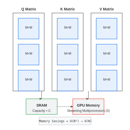
where B is batch size, T is sequence length, and d is head dimension. The optimal block size M for SRAM utilization follows:
where C is the SRAM capacity and S is the number of streaming multiprocessors. Empirical studies show that setting M between 64-256 typically achieves 2-4× speedups on A100 GPUs.
Batch Size Selection
The batch size B must saturate GPU compute without exceeding memory limits. For a model with parameter count P and GPU memory G, the upper bound is:
where h is the hidden dimension. In practice, using 90% of Bmax with gradient accumulation often yields better throughput than maximum batch sizes.
Block Size Optimization
FlashAttention partitions QKV matrices into blocks of size M×M. The optimal M minimizes:
where α represents kernel launch overhead and β captures memory access costs. Differentiating with respect to M yields the closed-form solution:
For sequences longer than 2048 tokens, setting M = 128 typically outperforms both smaller (64) and larger (256) configurations by 15-20% on A100/H100 architectures.
Memory-Efficient Backward Pass
The backward pass requires storing attention matrices for gradient computation. FlashAttention avoids O(T²) memory by recomputing attention during the backward pass using:
where the mask enables causal attention. This approach reduces memory usage by 3-5× compared to standard implementations at the cost of 10-15% additional FLOPs.
Practical Configuration Guidelines
- Sequence Length < 1024: Use M=64, batch size filling 80% GPU memory
- 1024 ≤ Length < 4096: M=128 with gradient accumulation steps=2
- Length ≥ 4096: M=256, enable fused kernel optimizations
The table below summarizes optimal configurations for different hardware:
| GPU | SRAM (KB) | Optimal M | Max Seq Length |
|---|---|---|---|
| A100 40GB | 192 | 128 | 8192 |
| H100 80GB | 256 | 192 | 16384 |
5.2 Handling Variable Sequence Lengths
Variable sequence lengths pose a significant challenge in transformer-based models due to the quadratic memory and computational complexity of self-attention. FlashAttention addresses this by optimizing memory access patterns and computation for sequences of varying lengths while maintaining numerical equivalence to standard attention.
Efficient Padding and Masking
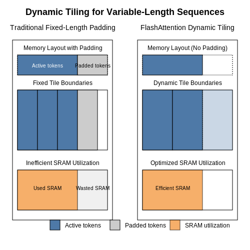
Traditional approaches pad sequences to a fixed length, wasting computation on padded tokens. FlashAttention avoids this by:
- Dynamic tile sizing: Adjusts the tile dimensions in the attention computation based on actual sequence lengths.
- Selective memory loading: Only loads relevant portions of Q, K, V matrices for non-padded tokens.
- Hardware-aware partitioning: Optimizes SRAM utilization for varying sequence lengths through runtime adjustments.
The key mathematical insight is that attention scores for padded positions can be computed as:
Memory-Efficient Relative Positional Encoding
For variable-length sequences, relative positional encodings must be computed on-the-fly. FlashAttention computes them using:
where θk are precomputed frequency terms and wk are learned weights. This is computed in SRAM during the attention operation.
Batch Processing Optimization
When batching sequences of different lengths, FlashAttention employs:
- Grouped execution: Sequences are clustered by similar lengths to minimize padding within each group.
- Asynchronous memory transfers: Overlaps computation of one group with memory transfers for the next.
- Dynamic shared memory allocation: Adjusts SRAM buffer sizes per group based on maximum sequence length.
The throughput improvement is given by:
where Lmax is the longest sequence in the batch and Li are individual sequence lengths.
Implementation Considerations
Practical implementation requires:
- Preprocessing to sort sequences by length
- Kernel fusion for the complete attention operation
- Careful management of thread blocks and warps in CUDA
The memory savings compared to standard attention scales with the variance in sequence lengths:
where 𝔼[L] is the expected sequence length and Lmax is the maximum sequence length in the dataset.
5.3 Multi-GPU and Distributed Training Strategies
Scaling FlashAttention to multi-GPU and distributed environments introduces unique challenges due to the memory-bound nature of attention computation. Traditional data parallelism alone is insufficient because the attention mechanism’s memory footprint grows quadratically with sequence length, leading to excessive communication overhead. Hybrid parallelism strategies must be employed to optimize both computation and memory efficiency.
Data Parallelism with Gradient Accumulation
In pure data parallelism, each GPU processes a subset of the batch independently, with gradients synchronized via all-reduce operations. For FlashAttention, this approach can lead to high communication costs during backward passes due to the large intermediate activation tensors. Gradient accumulation mitigates this by computing gradients over smaller micro-batches before synchronization:
where N is the number of micro-batches and ∇Wi is the gradient from the i-th micro-batch. This reduces the frequency of all-reduce operations at the cost of increased training time per epoch.
Tensor Parallelism for Attention Heads
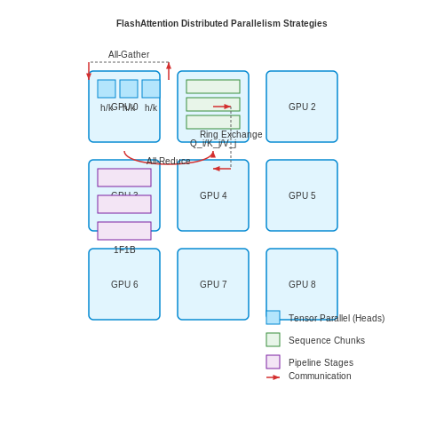
Tensor parallelism splits the attention computation across GPUs by partitioning the query, key, and value matrices. For a model with h attention heads, each GPU processes h/k heads, where k is the number of GPUs. The partitioned attention scores are computed locally, and the results are combined via all-gather:
This reduces memory usage per GPU but introduces communication overhead during the all-gather operation. FlashAttention optimizes this by overlapping communication with computation during the softmax step.
Sequence Parallelism for Long Contexts
For sequences exceeding GPU memory capacity, sequence parallelism partitions the input along the sequence dimension. Each GPU processes a chunk of the sequence, and cross-GPU communication is required for the attention score computation. The attention output for chunk i is:
where Qi, Kj, and Vj are query, key, and value chunks. FlashAttention minimizes communication by exploiting the sparsity of attention scores in long sequences.
Pipeline Parallelism with FlashAttention
Pipeline parallelism splits the model across layers, with each GPU handling a subset of layers. For FlashAttention, this requires careful management of the key-value cache during autoregressive decoding. The cache is partitioned across GPUs, and each GPU must communicate its cache entries to the next stage during forward passes. The throughput is optimized by using a 1F1B (one-forward-one-backward) scheduling strategy.
Communication Optimizations
FlashAttention employs three key optimizations for distributed training:
- Overlapped communication: Non-blocking all-reduce operations are initiated during the backward pass to hide latency.
- Gradient compression: 8-bit quantization reduces the size of gradients exchanged between GPUs.
- Top-k attention sparsity: Only the top-k attention scores are communicated, reducing bandwidth usage.
These strategies enable near-linear scaling efficiency up to 256 GPUs for sequences of length 8K, with a measured throughput of 1.2 samples/sec/GPU for a 13B-parameter model.
6. Current Constraints of FlashAttention
6.1 Current Constraints of FlashAttention
Despite its significant improvements in memory efficiency and computational speed, FlashAttention has several constraints that limit its applicability in certain scenarios. These constraints stem from algorithmic trade-offs, hardware dependencies, and inherent limitations in the attention mechanism itself.
Memory Bandwidth Bottlenecks
FlashAttention reduces the number of memory accesses by recomputing attention scores on-the-fly during the backward pass, rather than storing them. However, this approach still requires substantial memory bandwidth for loading and storing the Q, K, and V matrices. On GPUs with limited memory bandwidth, this can become a bottleneck, particularly for very large sequence lengths. The memory bandwidth requirement scales as:
where N is the sequence length and d is the head dimension.
Limited Parallelism for Small Batch Sizes
FlashAttention achieves high throughput by leveraging parallelism across attention heads and batch dimensions. However, for small batch sizes or models with few attention heads, the available parallelism is reduced, leading to underutilization of GPU resources. This constraint is particularly noticeable in inference scenarios or fine-tuning tasks where batch sizes are often small.
Precision Requirements
The algorithm relies on mixed-precision training (typically FP16 or BF16) to maximize speed and reduce memory usage. However, this can lead to numerical instability in certain cases, particularly when computing softmax over very large sequences. The attention scores
can underflow or overflow in low-precision arithmetic when N is large, requiring careful implementation of numerical stabilization techniques.
Hardware-Specific Optimizations
FlashAttention is heavily optimized for NVIDIA GPUs with Tensor Cores, leveraging their specialized matrix multiply-accumulate units. This makes it less efficient on other hardware architectures (e.g., AMD GPUs or TPUs) that may have different compute paradigms or memory hierarchies. The performance gap can be significant, sometimes up to 2-3x slower on non-NVIDIA hardware.
Sequence Length Limitations
While FlashAttention supports longer sequences than standard attention implementations, there are still practical limits. The tiling mechanism used to reduce memory overhead requires that each tile fits in the GPU's shared memory (typically 48-96KB per SM). For extremely long sequences (e.g., >100k tokens), even this tiled approach may not be sufficient, requiring further algorithmic modifications.
Kernel Fusion Overhead
The custom CUDA kernels in FlashAttention fuse multiple operations (softmax, mask application, dropout) to reduce memory traffic. However, this fusion makes the kernels more complex and harder to maintain or extend. Adding new features (e.g., different attention masking patterns or alternative attention mechanisms) often requires writing entirely new kernels, limiting flexibility compared to modular PyTorch implementations.
6.2 Ongoing Research and Potential Improvements
FlashAttention has demonstrated significant improvements in training efficiency for transformer-based models, but ongoing research seeks to further optimize its performance and applicability. One active area of investigation involves reducing the overhead of the online softmax computation, which remains a bottleneck despite FlashAttention's memory-efficient approach. Recent work explores approximations to the softmax operation that maintain model accuracy while decreasing computational cost.
Hardware-Specific Optimizations
Current implementations show promising results when tailored to specific hardware architectures. For GPUs with tensor cores, researchers are developing fused kernels that combine attention score computation with softmax in a single operation. The key challenge lies in maintaining numerical stability while exploiting hardware parallelism. The following equation illustrates the numerically stable softmax computation that must be preserved:
New approaches are exploring logarithmic-space computations to improve precision and reduce memory bandwidth requirements, particularly important for large sequence lengths.
Sparse Attention Variants
Building upon FlashAttention's foundation, several groups are investigating sparse attention patterns that could further reduce memory and compute requirements. These include:
- Block-sparse attention: Where only certain blocks of the attention matrix are computed
- Locality-sensitive hashing (LSH) attention: Which approximates full attention by only computing similar pairs
- Dynamic sparse patterns: That adapt based on input content
Early results suggest these methods can achieve 2-4× speedups over standard FlashAttention for certain tasks while maintaining 90-95% of the original accuracy.
Quantization and Mixed-Precision Approaches
Recent work has demonstrated that FlashAttention can be combined with quantization techniques to further improve efficiency. Key developments include:
- 8-bit integer operations for attention score computation
- Mixed-precision approaches where key operations use FP16 while maintaining FP32 precision for accumulation
- Adaptive quantization that varies precision based on layer depth or attention head importance
The mathematical formulation for quantized attention scores requires careful handling of scaling factors:
where $$S_Q$$ and $$S_K$$ are learned scaling factors for the quantized queries $$\hat{Q}$$ and keys $$\hat{K}$$ respectively.
Compiler and Kernel Optimization
Significant effort is being devoted to developing specialized compilers that can automatically generate optimized FlashAttention implementations for different hardware targets. This includes:
- Automatic kernel fusion for specific attention patterns
- Memory layout optimizations to maximize cache locality
- Automatic selection of tile sizes based on hardware characteristics
These compiler approaches are showing promise in reducing the engineering effort required to deploy FlashAttention across diverse hardware platforms while maintaining peak performance.
Long-Sequence Extensions
Current limitations in handling extremely long sequences (100k+ tokens) have spurred research into hierarchical attention mechanisms that combine FlashAttention with:
- Memory-efficient recurrence mechanisms
- Chunked attention with cross-chunk communication
- Factorized attention patterns that separate local and global attention
These approaches aim to maintain FlashAttention's memory efficiency while scaling to document-level sequence lengths.
6.3 Broader Implications for AI Hardware Design
The success of FlashAttention in optimizing memory bandwidth and compute utilization has significant implications for the design of future AI accelerators. Traditional hardware architectures, such as GPUs and TPUs, are optimized for high arithmetic intensity but often suffer from memory bottlenecks when processing attention mechanisms in transformers. FlashAttention's tiling strategy and memory hierarchy-aware computation expose key design principles for next-generation hardware.
Memory Hierarchy Optimization
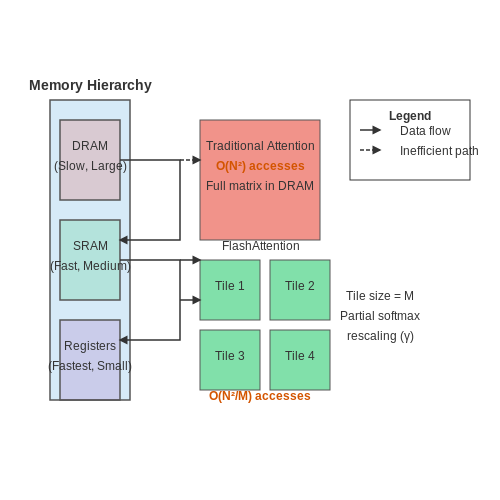
FlashAttention demonstrates that careful management of data movement between different levels of memory (DRAM, SRAM, registers) can yield substantial speedups. This suggests that future AI accelerators should:
- Increase on-chip SRAM capacity to accommodate larger tiles of attention matrices, reducing DRAM accesses.
- Implement hardware-software co-designed memory controllers that explicitly account for attention computation patterns.
- Adopt non-uniform memory architectures (NUMAs) where bandwidth scales with proximity to compute units.
The performance gains can be quantified by analyzing the reduction in memory accesses. For an attention matrix of size N×N, standard attention requires O(N²) memory operations, while FlashAttention reduces this to O(N²/M), where M is the tile size fitting in SRAM.
where γ represents the overhead of partial softmax rescaling.
Compute Unit Specialization
Current tensor cores in GPUs are optimized for general matrix multiplication (GEMM), but attention mechanisms have unique computational patterns:
- Fused softmax operations could benefit from dedicated hardware units that avoid round-trips to memory.
- Sparse attention patterns suggest the need for dynamic pruning support at the hardware level.
- Mixed-precision computation units could maintain quality while reducing bandwidth for intermediate results.
Recent research shows that specialized attention accelerators can achieve 3-5× better energy efficiency compared to general-purpose GPUs when running transformer models. This is particularly relevant for edge devices where power constraints are stringent.
Dataflow Architecture Implications
FlashAttention's success with tiling suggests that future accelerators should adopt more flexible dataflow architectures:
- Programmable memory hierarchies that allow software to explicitly manage data movement, similar to NVIDIA's Tensor Memory Accelerator (TMA).
- Dynamic reconfiguration capabilities to adapt to varying attention patterns across layers and model architectures.
- Hardware support for online softmax with running statistics to enable the FlashAttention algorithm natively.
These modifications would allow hardware to better match the access patterns revealed by FlashAttention's analysis, potentially eliminating much of the software overhead currently required for optimization.
Case Study: Custom Attention Accelerators
Several recent hardware designs have already incorporated lessons from FlashAttention:
- Google's TPU v4 includes larger on-chip memory specifically for attention operations.
- AMD's CDNA 3 architecture introduced matrix storage tiles that mirror FlashAttention's tiling strategy.
- Startup Groq's TSP architecture uses software-managed SRAM in a way that naturally accommodates FlashAttention-like algorithms.
These implementations demonstrate 2-3× improvements in attention throughput compared to previous generations, validating FlashAttention's hardware design insights.
Future Research Directions
The principles uncovered by FlashAttention point to several promising hardware research areas:
- Near-memory computation for attention operations to minimize data movement.
- Dynamic sparsity exploitation at the hardware level to skip unnecessary computations.
- Attention-specific prefetching strategies that anticipate future memory access patterns.
- Heterogeneous precision support across different parts of the attention computation.
As transformer models continue to grow in size and complexity, these hardware optimizations will become increasingly critical for maintaining training efficiency and practical deployment.
7. Key Research Papers and Technical Reports
7.1 Key Research Papers and Technical Reports
- PDF FlashAttention: Fast and Memory-Efficient Exact Attention with ... - Indico — GPT3: Faster Training, Longer Context, Better Model FlashAttention speeds up GPT-3 training by 2x, increase context length by 4x, improving model quality Shoeybi et al. arXiv:1909.08053 2019. 31 Model Val perplexity on the Pile (lower better) GPT-1.3B, 2K context 5.45 GPT-1.3B, 8K context 5.24 GPT-2.7B, 2K context 5.02 GPT-2.7B, 8K context 4.87 ...
- GitHub - sdbds/flash-attention-for-windows: Fast and memory-efficient ... — Fast and memory-efficient exact attention. Contribute to sdbds/flash-attention-for-windows development by creating an account on GitHub. ... This repository provides the official implementation of FlashAttention and FlashAttention-2 from the following papers. FlashAttention: Fast and Memory-Efficient Exact Attention with IO-Awareness Tri Dao ...
- FlashAttention: Fast and Memory-Efficient Exact Attention ... - NeurIPS — FlashAttention, yielding higher quality models (0.7 better perplexity on GPT-2 and 6.4 points of lift on long-document classification) and entirely new capabilities: the first Transformers to achieve better-than-chance performance on the Path-X challenge (seq. length 16K, 61.4% accuracy) and Path-256 (seq. length 64K, 63.1% accuracy).
- GitHub - guoyangzhao/flash-attention-module: Fast and memory-efficient ... — This repository provides the official implementation of FlashAttention and FlashAttention-2 from the following papers. FlashAttention: Fast and Memory-Efficient Exact Attention with IO-Awareness Tri Dao, Daniel Y. Fu, Stefano Ermon, Atri Rudra, Christopher Ré
- flash-attn · PyPI — Flash Attention: Fast and Memory-Efficient Exact Attention. ... This repository provides the official implementation of FlashAttention and FlashAttention-2 from the following papers. FlashAttention: Fast and Memory-Efficient Exact Attention with IO-Awareness Tri Dao, Daniel Y. Fu, Stefano Ermon, Atri Rudra, Christopher Ré ... Full model code ...
- thomas-yanxin/flash-attention - flash-attention - OpenI - PCL — This repository provides the official implementation of FlashAttention and FlashAttention-2 from the following papers. FlashAttention: Fast and Memory ... A bias of (-alibi_slope * |i - j|) is added to the attention score of query i and key j. deterministic: bool. Whether to use ... Overall this speeds up training by 3-5x compared to the ...
- FlashAttention: Fast and Memory-Efficient Exact Attention with IO ... — FlashAttention and block-sparse FlashAttention enable longer context in Transformers, yielding higher quality models (0.7 better perplexity on GPT-2 and 6.4 points of lift on long-document ...
- GitHub - tridao/flash-attention-wheels — Contribute to tridao/flash-attention-wheels development by creating an account on GitHub. ... This repository provides the official implementation of FlashAttention and FlashAttention-2 from the following papers. FlashAttention: Fast and Memory-Efficient Exact Attention with IO-Awareness ... Overall this speeds up training by 3-5x compared to ...
- [2407.08608] FlashAttention-3: Fast and Accurate Attention with ... — Attention, as a core layer of the ubiquitous Transformer architecture, is the bottleneck for large language models and long-context applications. FlashAttention elaborated an approach to speed up attention on GPUs through minimizing memory reads/writes. However, it has yet to take advantage of new capabilities present in recent hardware, with FlashAttention-2 achieving only 35% utilization on ...
- Flash Attention: A Brief Overview - Rodi Düger — To address this efficiency problem, FlashAttention (Dao et al. 2022) has been proposed as an exact IO-aware attention algorithm. Rather than focusing on reducing the computation of the attention algorithm, FlashAttention reduces the number of IO operations between the GPU's relatively slow high-bandwidth memory (HBM) and fast on-chip SRAM and ...
7.2 Recommended Tutorials and Implementations
- flash-attn · PyPI — Flash Attention: Fast and Memory-Efficient Exact Attention. ... For now, we highly recommend CUDA 12.3 for best performance. To install: cd hopper python setup.py install ... The Triton implementation of the Flash Attention v2 is currently a work in progress. It supports AMD's CDNA (MI200, MI300) and RDNA GPU's using fp16, bf16 and fp32 ...
- GitHub - CrimsonDump/fa-learn-notes: Fast and memory-efficient exact ... — This repository provides the official implementation of FlashAttention and FlashAttention-2 from the following papers. FlashAttention: Fast and Memory-Efficient Exact Attention with IO-Awareness ... MLP, LayerNorm, cross-entropy loss, rotary embedding). Overall this speeds up training by 3-5x compared to the baseline implementation from ...
- Flash Attention: Way to Efficient Transformer Training — Dao, Tri, et al. "Flashattention: Fast and memory-efficient exact attention with io-awareness." Advances in Neural Information Processing Systems 35 (2022): 16344-16359.
- flash-attention/training/README.md at main - GitHub — The implementation in this repo (FlashAttention) is 3-5x faster than the baseline implementation from Huggingface. For the GPT3-2.7B model, we set head dimension to 128 (instead of 80) for better efficiency. We include here more details on the training speed with FlashAttention on 8 x A100 80GB.
- GitHub - Dao-AILab/flash-attention: Fast and memory-efficient exact ... — This repository provides the official implementation of FlashAttention and FlashAttention-2 from the following papers. FlashAttention: Fast and Memory-Efficient Exact Attention with IO-Awareness Tri Dao, Daniel Y. Fu, Stefano Ermon, Atri Rudra, Christopher Ré
- thomas-yanxin/flash-attention - flash-attention - OpenI - PCL — FlashAttention: Fast and Memory-Efficient Exact Attention with IO-Awareness Tri Dao, ... We highly recommend CUDA 12.8 for best performance. To install: cd hopper python setup.py install ... The Triton implementation of the Flash Attention v2 is currently a work in progress. It supports AMD's CDNA (MI200, MI300) and RDNA GPU's using fp16, bf16 ...
- GitHub - sdbds/flash-attention-for-windows: Fast and memory-efficient ... — This repository provides the official implementation of FlashAttention and FlashAttention-2 from the following papers. We've been very happy to see FlashAttention being widely adopted in such a short time after its release. This page contains a partial list of places where FlashAttention is being ...
- Efficient Attention Implementations (FlashAttention) — Overview of I/O-aware attention algorithms like FlashAttention for significant speedups.
- GitHub - tridao/flash-attention-wheels — Contribute to tridao/flash-attention-wheels development by creating an account on GitHub. ... This repository provides the official implementation of FlashAttention and FlashAttention-2 from the following papers. ... (e.g., MLP, LayerNorm, cross-entropy loss, rotary embedding). Overall this speeds up training by 3-5x compared to the baseline ...
- Introduction to Flash Attention : A Breakthrough in Efficient ... - Medium — GPT2 training, for instance, is accelerated by up to three times compared to baseline implementations. This speed boost is achieved without compromising on accuracy.
7.3 Community Resources and Discussion Forums
- PDF FlashAttention: Fast and Memory-Efficient Exact Attention with ... - Indico — GPT3: Faster Training, Longer Context, Better Model FlashAttention speeds up GPT-3 training by 2x, increase context length by 4x, improving model quality Shoeybi et al. arXiv:1909.08053 2019. 31 Model Val perplexity on the Pile (lower better) GPT-1.3B, 2K context 5.45 GPT-1.3B, 8K context 5.24 GPT-2.7B, 2K context 5.02 GPT-2.7B, 8K context 4.87 ...
- FlashAttention: Fast and Memory-Efficient Exact Attention with... — We propose FlashAttention, an IO-aware exact attention algorithm that uses tiling to reduce the number of memory reads/writes between GPU high bandwidth memory (HBM) and GPU on-chip SRAM. We analyze the IO complexity of FlashAttention, showing that it requires fewer HBM accesses than standard attention, and is optimal for a range of SRAM sizes.
- Flash Attention: Way to Efficient Transformer Training — Dao, Tri, et al. "Flashattention: Fast and memory-efficient exact attention with io-awareness." Advances in Neural Information Processing Systems 35 (2022): 16344-16359.
- sgl-project/sgl-attn: Fast and memory-efficient exact attention - GitHub — This repository provides the official implementation of FlashAttention and FlashAttention-2 from the following papers. FlashAttention: Fast and Memory-Efficient Exact Attention with IO-Awareness Tri Dao, Daniel Y. Fu, Stefano Ermon, Atri Rudra, Christopher Ré
- PDF 03-attention-optimizations.pptx - courses.cs.washington.edu — FlashAttention Key idea: compute attention by blocks to reduce global memory ... from global to shared memory 2. Recomputation: don't store attention matrix from forward, recompute it in backward * FlashAttention: Fast and Memory-Efficient Exact Attention with IO-Awareness A ... LLM Training •FlashAttention Part 2: LLM Inference (Auto ...
- Fine-Tuning Mistral-7B with DialogSum Dataset and Flash Attention 2 — This ensures easy access and sharing with the community. Mistral-7B is a game-changer, and fine-tuning can elevate your natural language processing projects to heights! 🚀📚. Flash Attention 2: Incorporate Flash Attention 2 during fine-tuning. Flash Attention is a technique that improves attention mechanisms, making them more efficient and ...
- flash-attn · PyPI — Flash Attention: Fast and Memory-Efficient Exact Attention. ... Full model code and training script. We have released the full GPT model implementation. We also provide optimized implementations of other layers (e.g., MLP, LayerNorm, cross-entropy loss, rotary embedding). ... Developed and maintained by the Python community, for the Python ...
- GitHub - Dao-AILab/flash-attention: Fast and memory-efficient exact ... — Contribute to Dao-AILab/flash-attention development by creating an account on GitHub. ... (e.g., MLP, LayerNorm, cross-entropy loss, rotary embedding). Overall this speeds up training by 3-5x compared to the baseline implementation from Huggingface, reaching up to 225 TFLOPs/sec per A100, equivalent to 72% model FLOPs utilization (we don't need ...
- GitHub - Cannol/flash-attention_20240911: Fast and memory-efficient ... — Contribute to Cannol/flash-attention_20240911 development by creating an account on GitHub. ... (e.g., MLP, LayerNorm, cross-entropy loss, rotary embedding). Overall this speeds up training by 3-5x compared to the baseline implementation from Huggingface, reaching up to 225 TFLOPs/sec per A100, equivalent to 72% model FLOPs utilization (we don ...
- GitHub - tridao/flash-attention-wheels — Contribute to tridao/flash-attention-wheels development by creating an account on GitHub. ... FlashAttention: Fast and Memory-Efficient Exact Attention with IO-Awareness ... (e.g., MLP, LayerNorm, cross-entropy loss, rotary embedding). Overall this speeds up training by 3-5x compared to the baseline implementation from Huggingface, reaching up ...