Graph Transformers in Molecule Modeling
1. Graph Representation in Molecular Structures
Graph Representation in Molecular Structures
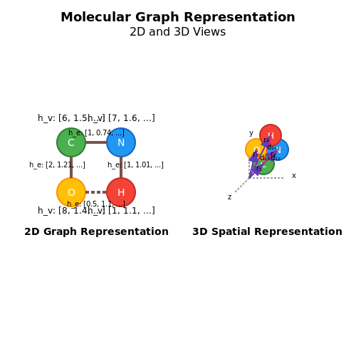
Molecular structures are naturally represented as graphs, where atoms correspond to nodes and chemical bonds to edges. This abstraction enables the application of graph-based machine learning techniques, such as graph neural networks (GNNs) and graph transformers, to model molecular properties and interactions. The graph representation captures both the topological connectivity and the physicochemical attributes of atoms and bonds.
Mathematical Formulation
A molecular graph G is formally defined as a tuple G = (V, E), where:
- V is the set of nodes (atoms), each represented by a feature vector hv encoding atomic properties such as element type, charge, and hybridization state.
- E is the set of edges (bonds), each represented by a feature vector he encoding bond type (single, double, triple), length, and aromaticity.
The adjacency matrix A encodes the connectivity:
Feature Engineering for Molecular Graphs
Node features typically include:
- Atomic number (one-hot encoded or embedded)
- Formal charge
- Number of bonded hydrogens
- Hybridization state (sp3, sp2, sp)
- Chirality
Edge features commonly incorporate:
- Bond type (single, double, triple, aromatic)
- Bond stereochemistry
- Conjugation
- Spatial distance (for 3D molecular graphs)
Extensions to 3D Molecular Structures
For 3D molecular modeling, the graph representation is augmented with spatial coordinates. Each node vi is assigned a position vector ri ∈ ℝ3, enabling the modeling of geometric constraints and non-bonded interactions. The edge features may then include:
where dij is the Euclidean distance between atoms i and j.
Graph Isomorphism and Molecular Fingerprints
The graph representation preserves molecular isomorphism - two molecules with identical connectivity are represented by isomorphic graphs. This property is leveraged in molecular fingerprinting algorithms like Morgan fingerprints, which generate invariant graph representations for similarity searching and clustering.
Modern graph-based approaches extend these concepts by learning continuous, task-specific molecular representations through differentiable graph operations, overcoming limitations of fixed fingerprint schemes.
Practical Considerations
In real-world applications, molecular graphs often require preprocessing:
- Hydrogen suppression (removing explicit hydrogen atoms to reduce graph size)
- Bond order normalization
- Special handling of disconnected components (salts, solvent molecules)
- Graph size normalization (padding/truncation for batch processing)
Transformer Architecture: Key Components
Self-Attention Mechanism
The self-attention mechanism computes a weighted sum of input representations, where the weights are dynamically derived based on pairwise interactions between all elements in the sequence. Given input embeddings X ∈ ℝn×d (where n is sequence length and d is embedding dimension), the queries (Q), keys (K), and values (V) are computed as:
where WQ, WK, WV ∈ ℝd×dk are learnable projection matrices. The attention scores are then calculated using scaled dot-product attention:
The scaling factor 1/√dk prevents gradient vanishing issues for large dk. Multi-head attention extends this by concatenating outputs from h parallel attention heads, enabling the model to jointly attend to information from different representation subspaces.
Positional Encoding
Since transformers lack recurrent or convolutional operations, positional encodings inject information about token positions into the input embeddings. For position pos and dimension i, the sinusoidal encoding is:
These encodings are added to the input embeddings before the first transformer layer. Recent variants like learned positional embeddings or relative position biases have shown improved performance in graph-based tasks where spatial relationships are non-sequential.
Layer Normalization and Residual Connections
Each sub-layer (attention or feed-forward) in the transformer employs residual connections followed by layer normalization:
This architecture mitigates vanishing gradients in deep networks. The layer normalization operates over the embedding dimension d, computing mean and variance for each token independently:
where μ, σ are the mean and standard deviation, and γ, β are learnable parameters.
Feed-Forward Networks
Each transformer layer contains a position-wise feed-forward network (FFN) applied identically to each token:
where W1 ∈ ℝd×dff, W2 ∈ ℝdff×d, and dff is typically 4×d. The FFN enables non-linear transformations of token representations independent of sequence position.
Graph Adaptations for Molecular Modeling
When applied to molecular graphs, transformers require modifications to handle non-sequential data:
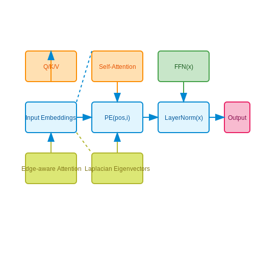
- Edge-aware attention: Attention scores incorporate bond information via additive terms in the QKT computation.
- Graph positional encodings: Laplacian eigenvectors or random walk probabilities replace sinusoidal encodings to capture graph topology.
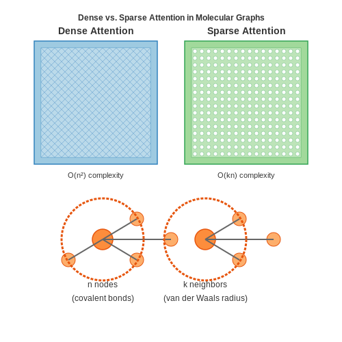
- Sparse attention: Attention matrices are masked to respect molecular connectivity, reducing computation from O(n2) to O(n) for sparse graphs.
1.3 Adapting Transformers for Graph Data
Standard Transformer architectures assume sequential inputs, making them incompatible with graph-structured data where relationships are non-Euclidean and permutation-invariant. Three key modifications enable Transformers to process graphs effectively: graph-aware positional encodings, structural attention biases, and edge feature integration.
Graph Positional Encodings
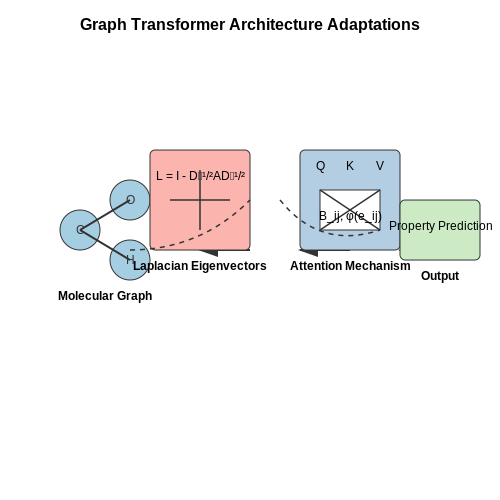
Traditional sinusoidal positional encodings are replaced with graph Laplacian eigenvectors or random walk probabilities to capture node centrality and connectivity patterns. For a graph with adjacency matrix A and degree matrix D, the normalized Laplacian eigenvectors provide spectral coordinates:
The eigenvectors corresponding to the smallest eigenvalues form a low-dimensional embedding that preserves graph topology. These replace token positions in the Transformer's input layer.
Attention with Structural Biases
The self-attention mechanism is augmented with a bias term Bij representing graph structure:
Common bias formulations include:
- Shortest path distance: Bij = -∞ for disconnected nodes
- Edge type embeddings: Learned vectors for different bond types
- Graph kernels: Diffusion-based or Weisfeiler-Lehman similarity scores
Edge Feature Integration
Molecular graphs require explicit handling of edge attributes (bond orders, spatial distances). The attention mechanism extends to incorporate edge features eij through:
Where φ is a learned linear or MLP projection. This allows simultaneous reasoning about node states and edge properties during message passing.
Practical Implementation
In PyTorch, these adaptations manifest as modified attention layers:
class GraphAttentionLayer(nn.Module):
    def __init__(self, hidden_dim, num_heads):
        super().__init__()
        self.edge_proj = nn.Linear(edge_dim, num_heads)
        self.query = nn.Linear(hidden_dim, hidden_dim)
        self.key = nn.Linear(hidden_dim, hidden_dim)

    def forward(self, x, edges, adj_matrix):
        Q = self.query(x)
        K = self.key(x)
        attn_scores = Q @ K.transpose(-2,-1) / np.sqrt(hidden_dim)
        attn_scores += adj_matrix.unsqueeze(1)  # Graph bias
        attn_scores += self.edge_proj(edges)    # Edge features
        return torch.softmax(attn_scores, dim=-1) @ V
This architecture forms the basis for molecular property prediction in frameworks like GROVER and GraphGPS, achieving state-of-the-art results on QM9 and MoleculeNet benchmarks by modeling long-range interactions beyond traditional GNNs.
2. Encoding Molecular Graphs with Transformers
2.1 Encoding Molecular Graphs with Transformers
Molecular graphs represent chemical structures as nodes (atoms) and edges (bonds), but traditional graph neural networks (GNNs) struggle with long-range dependencies due to their reliance on localized message passing. Transformers, with their self-attention mechanisms, overcome this limitation by enabling direct interactions between all atom pairs, regardless of distance. The key challenge lies in adapting the Transformer architecture to respect the inherent symmetries and physical constraints of molecular graphs.
Graph Representation for Transformer Input
To encode a molecular graph G = (V, E) into Transformer-compatible inputs, we define:
- Node features: Each atom v ∈ V is represented by a feature vector hv(0) containing atomic number, formal charge, hybridization state, and other quantum chemical properties.
- Edge features: Each bond (u,v) ∈ E is encoded as euv with bond type, length, and stereochemistry.
- Positional encodings: Unlike sequences, graphs lack inherent ordering. We use Laplacian eigenpositional encodings or random walk probabilities to inject structural information.
where λi, ϕi are the eigenvalues and eigenvectors of the graph Laplacian.
Attention with Edge-aware Bias
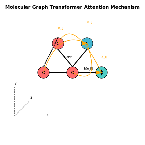
Standard self-attention computes pairwise attention scores without considering edge connectivity. For molecular graphs, we modify the attention mechanism to incorporate edge features:
where b(eij) is an edge-dependent bias term implemented as an MLP. This allows the model to learn different attention patterns for single, double, and aromatic bonds while maintaining permutation equivariance.
3D Geometry Integration
For molecular property prediction, 3D spatial coordinates are often critical. We extend the attention mechanism to be geometry-aware:
where ri are atomic coordinates and fdist is a distance-based kernel (e.g., exponential or Bessel basis functions). This enables the model to learn both topological and spatial relationships simultaneously.
Practical Implementation Considerations
When implementing graph Transformers for molecules:
- Memory efficiency: Full self-attention scales as O(N2) with atom count. Techniques like linear attention or local attention windows are often necessary for large molecules.
- Batch processing: Molecules vary in size. Implement dynamic batching with attention masks and graph padding.
- Multi-task learning: Jointly predict multiple molecular properties (energy, dipole moment, etc.) by sharing the Transformer backbone with task-specific heads.
Attention Mechanisms in Molecular Graphs
Self-Attention for Molecular Graph Nodes
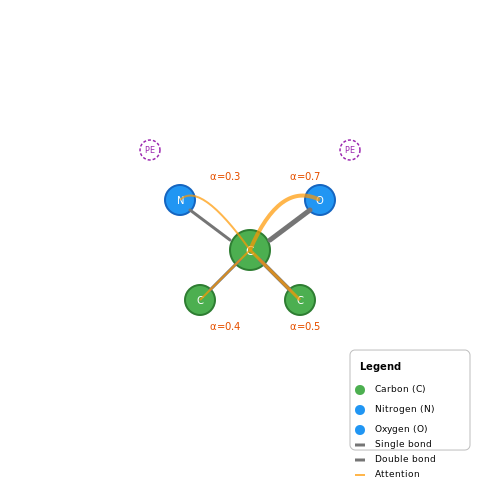
In graph transformers, self-attention operates on node features to capture long-range dependencies within molecular structures. Given a molecular graph G = (V, E) with node features X ∈ ℝn×d, where n is the number of atoms and d is the feature dimension, the attention mechanism computes pairwise interactions between all nodes.
Here, Q, K, and V are learned linear transformations of the input features:
The scaling factor √dk prevents gradient saturation in the softmax. For molecular graphs, this allows atoms to attend to chemically relevant distant neighbors beyond their immediate bonding environment.
Edge-Aware Attention in Molecular Graphs
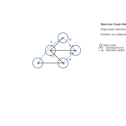
Standard self-attention treats all node pairs equally, ignoring bond information. Edge-aware attention incorporates bond types and distances through bias terms:
where bij encodes edge features between nodes i and j. Common implementations use:
- Bond type embeddings for discrete chemical bonds (single, double, aromatic)
- Continuous distance-based kernels for spatial relationships
- Combined geometric and chemical descriptors
Multi-Head Attention for Molecular Property Prediction
Multi-head attention extends the basic mechanism by applying h independent attention heads in parallel:
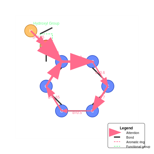
Each head learns different interaction patterns - some may focus on functional groups while others capture steric effects. For molecular property prediction, this proves particularly effective as evidenced by state-of-the-art results on QM9 and MoleculeNet benchmarks.
Spatial Attention in 3D Molecular Graphs
When 3D coordinates are available, attention mechanisms can incorporate spatial geometry through:
where ri are atomic positions and f is a distance-based function (e.g., Gaussian basis or learned MLP). This enables modeling of both chemical and geometric constraints, crucial for conformation-dependent properties.
Efficient Attention for Large Molecules
Standard attention's O(n2) complexity becomes prohibitive for large biomolecules. Recent approaches address this through:
- Linear attention approximations using kernel methods
- Local attention windows with chemical priors
- Hierarchical attention over molecular fragments
- Sparse attention patterns based on predicted relevance
These methods maintain performance while scaling to thousands of atoms, as demonstrated in protein-ligand interaction modeling.
2.3 Handling Variable-Sized Molecular Structures
Molecular graphs inherently possess variable sizes, with differing numbers of atoms (nodes) and bonds (edges). Traditional neural architectures struggle with this variability, as they typically require fixed-dimensional inputs. Graph Transformers address this challenge through several key mechanisms.
Dynamic Attention Masking
The self-attention mechanism in Transformers naturally handles variable sequence lengths, but requires careful masking for molecular graphs. For a molecule with N atoms, the attention scores Aij between atoms i and j are computed as:
where WQ and WK are learned query and key matrices, hi represents the embedding of atom i, and dk is the dimension of the key vectors. A binary mask M is applied element-wise to enforce attention only between connected atoms:
Positional Encodings for Graphs
Unlike sequential Transformers, graph Transformers require structural positional encodings. Common approaches include:
- Random Walk Positional Encodings (RWPE): Captures node proximity through random walk statistics
- Laplacian Eigenvectors: Uses the graph Laplacian's eigenvectors to encode structural roles
- Edge-aware Encodings: Incorporates bond distance and type information
The Laplacian-based approach computes positional encodings from the normalized graph Laplacian L = I - D-1/2AD-1/2, where A is the adjacency matrix and D is the degree matrix. The positional encoding for node i is given by:
where vk(i) is the i-th component of the k-th eigenvector, and αk are learned coefficients.
Hierarchical Pooling Strategies
For graph-level tasks, variable-sized graphs require pooling operations that preserve structural information. Two effective approaches are:
- Attention Pooling: Computes a weighted sum of node embeddings using learned attention scores
- Differentiable Pooling (DiffPool): Learns a soft assignment of nodes to clusters at each layer
The attention pooling operation computes the graph embedding hG as:
where Wa is a learned attention weight matrix, and ⊙ denotes element-wise multiplication.
Edge Feature Integration
Molecular bonds carry critical information (type, length, stereochemistry) that must be incorporated into the attention mechanism. The edge-augmented attention score becomes:
where eij represents the edge features between atoms i and j, and WE is a learned edge transformation matrix.
Recent advancements like GraphGPS (Rampášek et al., 2022) combine these approaches, using both structural encodings and edge features while maintaining permutation invariance. The architecture achieves this through a hybrid message-passing and attention mechanism that scales linearly with graph size.