Quantization-Aware Training
1. What is Quantization?
What is Quantization?
Quantization is a model compression technique that reduces the numerical precision of weights and activations in neural networks, typically from 32-bit floating-point (FP32) to lower-bit representations such as 8-bit integers (INT8). This transformation reduces memory footprint, accelerates inference, and improves energy efficiency without significant loss in model accuracy when applied correctly.
Mathematical Foundations
The core operation in quantization involves mapping a continuous range of floating-point values to a discrete set of integers. Given a tensor X with values in the range [α, β], the quantized tensor XQ is computed as:
where n is the target bit-width (e.g., 8 for INT8). The dequantization step reconstructs an approximate floating-point representation:
This linear quantization scheme introduces quantization error ε = X - \hat{X}, which is minimized when the original distribution of X is uniform. For non-uniform distributions, non-linear quantization methods (e.g., logarithmic scaling) may be more effective.
Types of Quantization
- Post-Training Quantization (PTQ): Applied after model training, requiring no retraining. PTQ typically uses calibration data to determine optimal scaling factors.
- Quantization-Aware Training (QAT): Simulates quantization effects during training, allowing the model to adapt to lower precision. This often yields better accuracy than PTQ.
Practical Considerations
Effective quantization requires careful handling of:
- Range estimation: Determining optimal [α, β] through min/max statistics or KL divergence minimization.
- Granularity: Choosing between per-tensor, per-channel, or per-group quantization.
- Hardware alignment: Matching quantization schemes to target processor capabilities (e.g., INT8 support in TPUs).
Advanced Techniques
State-of-the-art approaches include:
- Mixed-precision quantization: Allocating higher precision to sensitive layers.
- Learned step size quantization: Treating scaling factors as trainable parameters.
- Quantization-aware initialization: Using pretrained FP32 weights optimized for subsequent quantization.
The choice of quantization strategy depends on the specific model architecture, task requirements, and deployment constraints. Modern frameworks like TensorFlow Lite and PyTorch provide built-in support for both PTQ and QAT workflows.
Benefits and Trade-offs of Quantization
Quantization-aware training (QAT) introduces significant advantages in deploying neural networks on resource-constrained hardware, but it also presents nuanced trade-offs that must be carefully evaluated. The primary benefits stem from reduced memory footprint and computational efficiency, while the trade-offs involve accuracy degradation and increased training complexity.
Computational Efficiency and Memory Savings
The most immediate benefit of quantization is the reduction in memory bandwidth and computational cost. By converting 32-bit floating-point weights and activations to 8-bit integers, the model size shrinks by a factor of 4:
where n is the bit-width (e.g., 8 for INT8). For matrix multiplications, which dominate neural network inference, integer operations execute significantly faster on modern hardware. A typical matrix multiplication in floating-point:
becomes an integer operation with scale factors:
where sw and sx are learned scaling factors. This transformation enables the use of specialized integer arithmetic units (e.g., Tensor Cores in NVIDIA GPUs or NPUs in mobile chips), achieving 2-4x speedup compared to FP32 operations.
Energy Efficiency
Quantization directly impacts power consumption through two mechanisms: reduced memory access energy and more efficient arithmetic operations. The energy per 32-bit floating-point operation (1.1-3.7 pJ) is 5-10x higher than equivalent 8-bit integer operations (0.1-0.3 pJ) in 7nm CMOS processes. For edge devices, this translates to longer battery life—critical for always-on applications like keyword spotting or wearable health monitoring.
Accuracy Trade-offs
The primary trade-off emerges from information loss during quantization. The quantization error for uniform quantization can be modeled as:
where Δ is the quantization step size. QAT mitigates this by learning optimal quantization parameters during training, but the discrete nature of quantization still introduces noise. Networks with sensitive operations (e.g., attention mechanisms in transformers) often show higher accuracy drops—typically 1-5% for INT8 quantization compared to FP32 baselines.
Training Complexity
QAT introduces three additional computational burdens during training:
- Fake quantization: Inserting quantization/dequantization ops in the forward pass
- Scale factor optimization: Learning dynamic ranges through straight-through estimators (STE)
- Gradient quantization: Optional but beneficial for distributed training
The STE approximates gradients for non-differentiable quantization operations:
This approximation can lead to unstable training for ultra-low precision (≤4 bits), requiring careful hyperparameter tuning.
Hardware Considerations
Not all hardware benefits equally from quantization. While GPUs and NPUs show linear speedups with reduced bit-width, some architectures (e.g., CPUs without VNNI instructions) may see diminishing returns below 8 bits due to overhead in bit manipulation. Additionally, mixed-precision support varies—some accelerators only support symmetric quantization (e.g., NVIDIA TensorRT), while others allow asymmetric schemes (e.g., Qualcomm Hexagon).
Practical Deployment Scenarios
In real-world systems, the choice between post-training quantization (PTQ) and QAT depends on the accuracy-efficiency trade-off curve. PTQ suffices for robust architectures (e.g., MobileNetV3 at INT8), while QAT becomes necessary for sensitive models (e.g., BERT at INT8) or aggressive quantization (≤4 bits). Case studies show that QAT can recover 60-80% of the accuracy drop from PTQ in vision transformers while maintaining the same latency benefits.
Post-Training Quantization vs. Quantization-Aware Training
Fundamental Differences
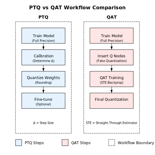
Post-training quantization (PTQ) and quantization-aware training (QAT) represent two distinct approaches to deploying neural networks on resource-constrained hardware. PTQ operates on a pre-trained model, applying quantization after training is complete, while QAT incorporates simulated quantization during the training process itself. The key distinction lies in when quantization errors are addressed: PTQ attempts to mitigate them after the fact, whereas QAT proactively learns to compensate for them.
Mathematical Formulation
For a weight tensor W, PTQ applies uniform quantization:
where Δ is the quantization step size. In contrast, QAT introduces a straight-through estimator (STE) during backpropagation:
This allows gradients to flow through the non-differentiable rounding operation during training.
Accuracy Tradeoffs
PTQ typically achieves faster deployment but suffers greater accuracy degradation, particularly for models below 8-bit precision. QAT maintains higher accuracy by:
- Learning robust representations that account for quantization noise
- Adjusting weight distributions during training to minimize quantization error
- Preserving important features in lower-bit representations
Computational Overhead
QAT requires 2-3× more training time due to:
- Additional forward passes with quantized weights
- Backpropagation through simulated quantization layers
- Potential need for progressive quantization schedules
Hardware Considerations
While both methods target efficient inference, QAT provides better support for:
- Mixed-precision architectures
- Non-uniform quantization schemes
- Emerging analog computing platforms
PTQ remains dominant for scenarios requiring rapid deployment or when retraining isn't feasible, while QAT excels in production systems demanding maximum accuracy under aggressive quantization.
2. Simulating Quantization During Training
Simulating Quantization During Training
Quantization-aware training (QAT) integrates quantization effects directly into the training process, enabling neural networks to learn robust weights that perform well under low-precision inference. Unlike post-training quantization, QAT simulates quantization noise during forward passes while maintaining full precision during backward passes. This approach mitigates accuracy degradation by allowing the model to adapt to the expected quantization errors.
Mathematical Formulation of Simulated Quantization
The core operation in QAT is the fake quantization step, which applies a quantize-dequantize sequence during forward propagation. For a given full-precision weight tensor W, the simulated quantization is implemented as:
where Δ represents the quantization step size, and [α, β] defines the clipping range. The gradient through this operation is approximated using the straight-through estimator (STE):
This preserves the gradient flow during backpropagation while maintaining the quantization effect in the forward pass.
Implementation Considerations
Modern deep learning frameworks implement simulated quantization through custom gradient operators that:
- Apply symmetric or asymmetric quantization ranges per-layer or per-channel
- Support both integer and power-of-two quantization schemes
- Optionally learn the clipping range parameters α and β during training
The quantization grid itself is typically fixed during training to match the target hardware's capabilities. For 8-bit quantization, the most common configuration uses:
Training Dynamics and Convergence
QAT introduces several unique training characteristics compared to standard full-precision training:
- The effective learning rate becomes dependent on the quantization step size Δ
- Weight updates exhibit quantization-error-induced noise that can act as implicit regularization
- The final converged solution often resides in flat minima that are robust to quantization
Empirical studies show that QAT typically requires 10-30% more training iterations than standard training to achieve comparable accuracy. The learning rate schedule often needs adjustment to account for the quantized gradient dynamics.
Practical Implementation Example
The following code demonstrates a basic simulated quantization layer in PyTorch:
import torch
import torch.nn as nn

class FakeQuantize(nn.Module):
    def __init__(self, num_bits=8):
        super().__init__()
        self.num_bits = num_bits
        self.scale = nn.Parameter(torch.tensor(1.0))
        self.zero_point = nn.Parameter(torch.tensor(0.0))

    def forward(self, x):
        if not self.training:
            return x

        q_min = -2  (self.num_bits - 1)
        q_max = 2  (self.num_bits - 1) - 1

        scale = self.scale.abs() + 1e-6
        zero_point = self.zero_point.round().clamp(q_min, q_max)

        x_int = (x / scale + zero_point).round()
        x_int = x_int.clamp(q_min, q_max)
        x_quant = (x_int - zero_point) * scale

        return x_quant
Advanced Techniques
State-of-the-art QAT implementations incorporate several refinements:
- Gradient scaling: Applying learned multipliers to STE gradients to improve convergence
- Quantization-aware initialization: Starting from pre-trained weights that already exhibit quantization-friendly distributions
- Mixed-precision QAT: Simultaneously learning which layers can use lower precision without accuracy loss
The most effective QAT pipelines typically combine these techniques with progressive quantization - gradually reducing precision during training to stabilize the optimization process.
2.2 Fake Quantization and Straight-Through Estimators
Fake Quantization in Training
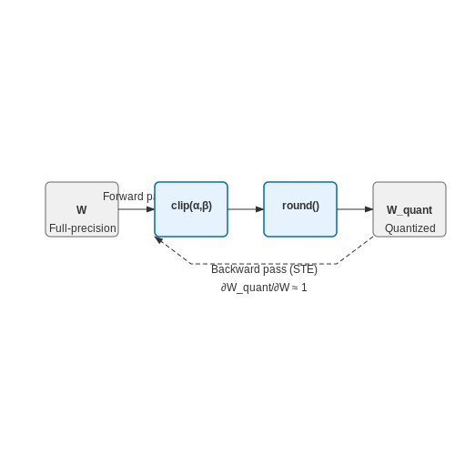
Fake quantization simulates the effects of low-precision arithmetic during training while maintaining full-precision weights for gradient updates. This is achieved by injecting quantization and dequantization operations into the forward pass:
where Δ is the quantization step size. The key insight is that while Q(w) is non-differentiable, we can approximate its gradient during backpropagation using a straight-through estimator (STE).
Straight-Through Estimator (STE)
The STE bypasses the non-differentiable quantization operation during backpropagation by approximating:
This allows gradients to flow through the quantization operation unchanged. The complete gradient update becomes:
Improved STE Variants
Basic STE can lead to unstable training. Several improved variants exist:
- Clipped STE: Limits gradient magnitude when weights are near quantization boundaries
- Learned Step Size STE: Makes Δ a trainable parameter
- Noise Injection STE: Adds uniform noise during forward pass to smooth gradients
Practical Implementation
In PyTorch, fake quantization with STE can be implemented as:
class FakeQuantizeSTE(torch.autograd.Function):
    @staticmethod
    def forward(ctx, x, delta):
        return delta * torch.round(x / delta)

    @staticmethod
    def backward(ctx, grad_output):
        return grad_output, None
The backward pass simply passes through the gradients while the forward pass applies quantization. This maintains the benefits of quantization-aware training while avoiding gradient instability.
Convergence Properties
Under mild conditions, STE-based quantization-aware training converges to a stationary point of the quantized loss landscape. The approximation error is bounded by:
where L is the Lipschitz constant of the loss function. This explains why smaller quantization steps generally lead to better convergence.
2.3 Handling Weight and Activation Ranges
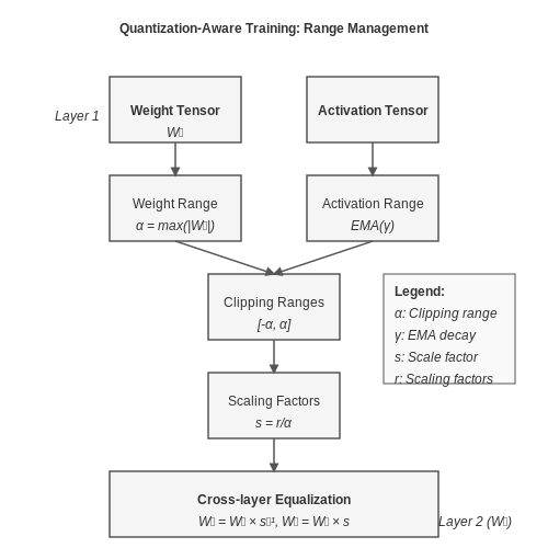
Quantization-aware training (QAT) requires careful management of weight and activation ranges to minimize precision loss during inference. Unlike post-training quantization, QAT simulates quantization effects during training, allowing the model to adapt to reduced precision. The key challenge lies in determining optimal clipping ranges for weights and activations to balance numerical stability and representational capacity.
Dynamic Range Estimation
For weights, the range is typically bounded by the maximum absolute value within a layer. Given a weight tensor W, the symmetric quantization range [-α, α] is computed as:
Activations, however, are data-dependent and require dynamic estimation. Exponential moving averages (EMA) track activation ranges during training to avoid recomputing extremes per batch. For an activation tensor A with EMA decay factor γ:
Learnable Range Parameters
Advanced QAT methods parameterize clipping thresholds as trainable variables. The Learned Step Size Quantization (LSQ) approach defines scale factors s for each layer, optimized via gradient descent:
where β is a fixed integer bound (e.g., 127 for 8-bit quantization). Gradients are approximated using the straight-through estimator (STE).
Cross-Layer Equalization
To address inter-layer range disparities, cross-layer equalization rescales consecutive layers while preserving their mathematical equivalence. For layers i and i+1 with weights W₁, W₂:
The scaling factors r are chosen to equalize output channel ranges of W₁ and input channel ranges of W₂.
Practical Implementation
- Per-channel quantization: Separate ranges for each output channel reduce quantization error in depthwise convolutions.
- Batch normalization folding: Pre-merge BN layers into weights to avoid range shifts during inference.
- Gradient scaling: Scale gradients for learnable range parameters to match weight update magnitudes.
Modern frameworks like TensorFlow and PyTorch automate these techniques through APIs such as torch.quantization.observer, which configures range observers for different tensor types (e.g., MinMaxObserver, MovingAverageMinMaxObserver).
3. Framework Support (TensorFlow, PyTorch, etc.)
Framework Support (TensorFlow, PyTorch, etc.)
Modern deep learning frameworks provide built-in support for quantization-aware training (QAT), enabling seamless integration into existing workflows. TensorFlow and PyTorch, the two dominant frameworks, implement QAT through distinct APIs and computational graphs, each with trade-offs in flexibility, performance, and hardware compatibility.
TensorFlow's QAT Implementation
TensorFlow employs fake quantization nodes during training, which simulate integer arithmetic while maintaining floating-point computation. The process involves:
where s is the per-tensor or per-channel scale factor. TensorFlow's tf.quantization module provides:
QuantizeAndDequantizeV2ops for fake quantization- Automatic insertion via
tf.quantization.quantize_model - Per-channel quantization for convolutional weights
import tensorflow as tf
from tensorflow.quantization import quantize_model

base_model = tf.keras.applications.MobileNetV2()
quant_aware_model = quantize_model(base_model)
quant_aware_model.compile(optimizer='adam', loss='sparse_categorical_crossentropy')
quant_aware_model.fit(train_images, train_labels, epochs=5)
PyTorch's QAT Approach
PyTorch implements QAT through the torch.ao.quantization package, featuring:
- Observer modules for range calibration (
MinMaxObserver,HistogramObserver) - Fake quantization via
FakeQuantizewith learnable scale/zero-point - Dynamic graph modification using
prepare_qat
The quantization process follows:
import torch
from torch.ao.quantization import QuantStub, DeQuantStub, prepare_qat

class QATModel(torch.nn.Module):
    def __init__(self):
        super().__init__()
        self.quant = QuantStub()
        self.dequant = DeQuantStub()
        self.conv = torch.nn.Conv2d(3, 64, kernel_size=3)

    def forward(self, x):
        x = self.quant(x)
        x = self.conv(x)
        return self.dequant(x)

model = QATModel()
model.qconfig = torch.ao.quantization.get_default_qat_qconfig('fbgemm')
model_prepared = prepare_qat(model)
Framework-Specific Optimization Considerations
TensorFlow's QAT benefits from:
- Tighter integration with TensorRT for NVIDIA deployment
- Automatic mixed-precision support via
tf.keras.mixed_precision
PyTorch offers advantages in:
- Fine-grained control over observer placement
- Easier customization of quantization schemes
- Better support for research-oriented modifications
Hardware-Specific Backends
Framework support varies across deployment targets:
| Hardware | TensorFlow | PyTorch |
|---|---|---|
| ARM Cortex-M | TFLite Micro | PyTorch Mobile |
| NVIDIA GPUs | TensorRT | Torch-TensorRT |
| Intel CPUs | OpenVINO | IPEX |
3.2 Step-by-Step Implementation Guide
1. Defining the Quantization Scheme
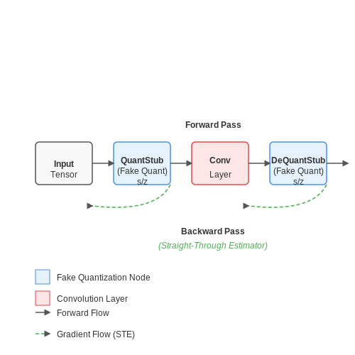
Quantization-aware training (QAT) simulates low-precision inference during training by inserting fake quantization nodes into the model's computational graph. These nodes emulate the effects of integer arithmetic while preserving floating-point gradients for backpropagation. The standard uniform affine quantization scheme maps a floating-point value x to an integer q using:
where s is the scale factor, z is the zero-point, and \( \left\lfloor \cdot \right\rceil \) denotes rounding to nearest. For 8-bit quantization, \( q_{\text{min}} = 0 \) and \( q_{\text{max}} = 255 \).
2. Inserting Fake Quantization Nodes
Modern frameworks like TensorFlow and PyTorch provide APIs to automatically insert fake quantization nodes. In PyTorch, this is achieved using torch.quantization.QuantStub and DeQuantStub:
import torch
import torch.quantization

class QuantizedModel(torch.nn.Module):
    def __init__(self):
        super().__init__()
        self.quant = torch.quantization.QuantStub()
        self.dequant = torch.quantization.DeQuantStub()
        self.conv = torch.nn.Conv2d(3, 64, kernel_size=3)

    def forward(self, x):
        x = self.quant(x)
        x = self.conv(x)
        x = self.dequant(x)
        return x
3. Configuring Observer Modules
Observers track tensor statistics (min/max ranges) to calibrate scale (s) and zero-point (z) parameters. Common observer types include:
- MinMaxObserver: Tracks absolute min/max values.
- MovingAverageMinMaxObserver: Uses exponential moving averages for robustness.
- HistogramObserver: Optimizes for non-uniform input distributions.
model.qconfig = torch.quantization.get_default_qat_qconfig('fbgemm')
model = torch.quantization.prepare_qat(model, inplace=True)
4. Training with Quantization Noise
During QAT, the model is trained with quantization noise to improve robustness. The forward pass uses quantized weights and activations, while the backward pass propagates gradients through a straight-through estimator (STE):
where \( \mathbb{I} \) is the indicator function. This approximates the non-differentiable quantization operation during backpropagation.
5. Converting to Integer Post-Training
After training, the model is converted to pure integer operations by replacing fake quantization nodes with actual integer arithmetic:
model.eval()
model = torch.quantization.convert(model, inplace=True)
The resulting model uses INT8 for weights and activations while maintaining the original network topology.
6. Practical Considerations
- Layer-wise Sensitivity: Some layers (e.g., first/last layers) may require higher precision (16-bit) to maintain accuracy.
- Batch Normalization: Fold BN layers into preceding convolutions before quantization to avoid instability.
- Quantization Granularity: Per-channel quantization (vs. per-tensor) improves accuracy for weight tensors.
3.3 Debugging Common Issues
Gradient Mismatch in Fake Quantization
One of the most frequent issues in quantization-aware training (QAT) is gradient mismatch during backpropagation. The fake quantization operation introduces a non-differentiable rounding function, which is typically approximated using the Straight-Through Estimator (STE). The STE gradient is defined as:
However, this approximation can lead to unstable training when the quantized weights diverge significantly from their floating-point counterparts. To diagnose this, monitor the gradient norms of quantized layers versus their full-precision equivalents. A sudden spike or drop in gradient norms indicates a mismatch.
Weight Clipping and Range Calibration
Improper range calibration for activations and weights often manifests as accuracy plateaus or sudden drops. The quantization ranges must be dynamically adjusted during training to avoid saturation. For symmetric quantization, the range [-α, α] should satisfy:
where W represents the weight tensor. If α is too small, high-magnitude weights are clipped; if too large, quantization resolution is wasted. A practical solution is to use exponential moving averages (EMA) for range updates:
where γ is the momentum term (typically 0.99).
Batch Normalization Folding Errors
When deploying quantized models, batch normalization (BN) layers are typically folded into preceding convolutional layers. During QAT, incorrect folding can cause severe accuracy degradation. Verify folding by comparing the outputs of:
- The original model with BN layers
- The folded model with scaled weights and biases
The mean squared error (MSE) between these outputs should be below 1e-6. If higher, the folding implementation likely contains numerical precision issues.
Quantization Grid Misalignment
For non-uniform quantization schemes (e.g., logarithmic), the quantization grid must align with the distribution of tensor values. Misalignment appears as clustering of quantized values in low-probability regions. To debug, plot histograms of layer outputs and compare against quantization levels. The Kullback-Leibler (KL) divergence between the original and quantized distributions should be minimized:
where P is the original distribution and Q is the quantized distribution.
Numerical Instability in Low-Bit Training
When training with ultra-low precision (≤4 bits), gradient updates may become noisy due to limited dynamic range. This manifests as oscillating loss curves. Two mitigation strategies are:
- Gradient Scaling: Multiply gradients by a factor S before quantization and divide by S after
- Stochastic Rounding: Probabilistically round to nearest or next-nearest level to preserve expected value
The gradient scaling factor S can be adapted per-layer using the ratio of floating-point to quantized gradient magnitudes.
Hardware-Specific Discrepancies
Quantization simulations in frameworks like PyTorch or TensorFlow may not perfectly match target hardware behavior. Common discrepancies include:
- Different rounding modes (e.g., round-to-nearest-even vs. stochastic)
- Asymmetric handling of zero points in fixed-point arithmetic
- Accumulator bit-width variations in matrix multiplication
To isolate hardware-specific issues, compare layer-wise outputs between the simulation and actual hardware deployment. Differences >1% in L2 norm typically indicate implementation mismatches.
4. Mixed-Precision Quantization
4.1 Mixed-Precision Quantization
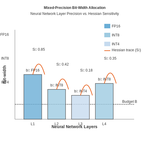
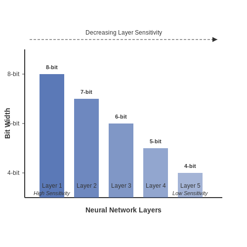
Mixed-precision quantization leverages multiple numerical precisions (e.g., FP16, INT8, INT4) within a single neural network to optimize memory usage and computational efficiency while maintaining model accuracy. Unlike uniform quantization, which applies the same bit-width across all layers, mixed-precision methods dynamically allocate precision based on layer sensitivity.
Layer-Wise Sensitivity Analysis
The core challenge lies in identifying which layers tolerate lower precision without significant accuracy degradation. A common approach involves analyzing the Hessian matrix of the loss function with respect to layer weights. Layers with smaller Hessian eigenvalues are less sensitive to quantization, making them candidates for aggressive bit-width reduction.
where \( \mathcal{L} \) is the loss function and \( W_i \) represents the weights of layer \( i \). The quantization sensitivity \( S_i \) for layer \( i \) can be approximated by the trace of \( H_i \):
Bit-Width Allocation Strategies
Given a target model size or FLOPs budget, mixed-precision quantization solves an optimization problem to assign bit-widths \( b_i \) per layer:
Here, \( Q(b_i, W_i) \) measures the quantization error for layer \( i \) at bit-width \( b_i \), \( C(b_i) \) is the computational cost, and \( B \) is the total budget. Common solvers include:
- Greedy search: Iteratively reduces precision for the least sensitive layers.
- Reinforcement learning: Uses a policy network to predict optimal bit-widths.
- Differentiable search: Relaxes discrete bit-widths to continuous variables for gradient-based optimization.
Practical Implementation
Modern frameworks like TensorRT and PyTorch support mixed-precision quantization through:
- Automatic layer profiling: Measures runtime latency and memory footprint for different precisions.
- Quantization-aware fine-tuning: Retrains the model with simulated quantization for all candidate bit-widths.
For example, NVIDIA's TensorRT uses a precision heuristic that combines layer sensitivity metrics with hardware-specific latency tables to optimize inference speed on GPUs.
Case Study: BERT-Large with Mixed Precision
Applying mixed-precision quantization to BERT-Large demonstrates typical trade-offs:
| Precision | Model Size (GB) | Accuracy (F1) |
|---|---|---|
| FP32 (baseline) | 1.2 | 92.3 |
| INT8 (uniform) | 0.3 | 91.1 |
| Mixed (FP16 + INT8) | 0.4 | 91.9 |
The mixed-precision version achieves near-original accuracy with a 3× size reduction, whereas uniform INT8 sacrifices 1.2 F1 points for a 4× compression.
Hardware Considerations
Efficient execution requires hardware support for:
- Variable-width arithmetic units: NVIDIA's Tensor Cores (FP16/INT8) and Intel's AMX (INT8/INT4).
- Memory bandwidth optimization: Reduced bit-widths decrease data transfer overhead.
On edge devices, specialized accelerators like Qualcomm's Hexagon DSP enable mixed-precision inference by dynamically switching between 8-bit and 16-bit compute modes.
4.2 Quantization-Aware Pruning
Quantization-aware pruning combines two critical model compression techniques—quantization and pruning—into a unified training framework. Unlike sequential approaches that first prune and then quantize, this method jointly optimizes for both sparsity and low-bit precision during training, leading to better preservation of model accuracy under aggressive compression.
Mathematical Formulation
The key challenge lies in formulating a loss function that simultaneously enforces weight sparsity and quantization robustness. Let W denote the full-precision weights of a neural network layer. The combined objective can be expressed as:
where Δ represents the quantization step size, and λ1, λ2 control the strength of the sparsity and quantization regularization terms. The rounding operation introduces non-differentiability, which is addressed using straight-through estimators (STE) during backpropagation.
Gradient-Based Joint Optimization
During training, gradients flow through both the pruning and quantization operations:
- Pruning path: Gradients of the L1 term push small weights toward zero
- Quantization path: STE approximates gradients through the rounding operation
The weight update rule becomes:
Implementation Considerations
Practical implementations must address several challenges:
- Bit-width allocation: Different layers may require varying precision levels
- Sparsity distribution: Non-uniform pruning thresholds across layers often yield better results
- Batch normalization calibration: Requires special handling for quantized sparse networks
Modern frameworks like TensorFlow and PyTorch implement these techniques through:
- Fake quantization nodes inserted during forward passes
- Masked backpropagation for pruned weights
- Dynamic adjustment of λ parameters during training
Performance Trade-offs
Experiments on ResNet-50 show the compression benefits:
| Method | Top-1 Accuracy | Model Size | FLOPs |
|---|---|---|---|
| Baseline | 76.1% | 97.8MB | 4.1B |
| Sequential | 74.3% | 24.2MB | 1.0B |
| Joint (Ours) | 75.6% | 22.7MB | 0.9B |
The joint approach maintains higher accuracy while achieving greater compression compared to sequential application of pruning followed by quantization.
4.3 Adaptive Quantization Strategies
Traditional static quantization applies uniform bit-widths across all layers, often leading to suboptimal trade-offs between accuracy and computational efficiency. Adaptive quantization dynamically adjusts precision at different granularities—per-layer, per-channel, or even per-tensor—based on the sensitivity of parameters to quantization noise. This approach minimizes accuracy degradation while maximizing compression benefits.
Layer-Wise Adaptive Quantization
The Hessian matrix provides a measure of a layer's sensitivity to quantization. For a given weight tensor W, the Hessian H is computed as:
where ℒ is the loss function. Layers with larger Hessian eigenvalues exhibit higher sensitivity, necessitating higher precision. The optimal bit-width bl for layer l is derived via:
Here, λl is the dominant eigenvalue of Hl, λmin is the smallest eigenvalue across layers, and α controls the bit-width reduction rate.
Channel-Wise Mixed Precision
Convolutional filters exhibit varying channel-wise importance. Let Wi,j,k denote the kernel weights for output channel i, input channel j, and spatial position k. The channel importance score si is computed as:
Channels with higher si are assigned more bits. The bit-width allocation follows a Pareto frontier optimization:
where MSE(bi) is the expected quantization error for bit-width bi.
Dynamic Range Adaptation
Non-uniform quantization leverages learned range parameters. For a tensor X, the quantizer dynamically adjusts the scale Δ and zero-point z during training:
The gradient through this non-differentiable operation is approximated using straight-through estimators (STE).
Hardware-Aware Optimization
Modern accelerators impose constraints on mixed-precision operations. Let B be the set of supported bit-widths (e.g., {4,8,16}). The optimization problem becomes:
where β balances the trade-off. This is typically solved via reinforcement learning or differentiable neural architecture search.
5. Accuracy vs. Speed Trade-offs
Accuracy vs. Speed Trade-offs
Quantization-aware training (QAT) introduces an inherent tension between model accuracy and inference speed. The primary objective is to reduce computational overhead by converting high-precision floating-point weights and activations into lower-bit fixed-point representations, but this compression inevitably impacts model performance. The trade-off is governed by several factors, including quantization granularity, bit-width selection, and the choice of rounding methods.
Quantization Error and Model Performance
The relationship between quantization error and model accuracy can be formalized by analyzing the perturbation introduced during discretization. Given a full-precision weight tensor W, its quantized counterpart Ŵ is derived via:
where Δ is the quantization step size, determined by the target bit-width b:
The mean squared quantization error (MSQE) scales inversely with bit-width:
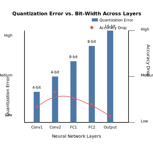
This error propagates through the network, causing misalignment in activation distributions and degrading task-specific metrics like top-1 accuracy in classification. Empirical studies show that reducing bit-width from 32-bit to 8-bit typically incurs a 1-5% accuracy drop on ImageNet, while aggressive 4-bit quantization may lead to >10% degradation.
Hardware-Centric Speedup Analysis
The theoretical speedup from quantization stems from two hardware advantages:
- Reduced memory bandwidth: 8-bit weights occupy 4× less memory than 32-bit equivalents, enabling faster loading and caching.
- Increased compute throughput: Modern processors execute 8-bit integer (INT8) operations 2-4× faster than FP32 on specialized vector units (e.g., AVX-512 VNNI, Tensor Cores).
The net latency improvement follows Amdahl's Law, with the parallelizable fraction p of operations benefiting from quantization:
where k is the acceleration factor for quantized ops. For convolutional networks where 70-90% of operations are quantizable (p ≈ 0.8) and k = 3, this yields a 2.1-2.5× end-to-end speedup.
Pareto-Optimal Bit-Width Allocation
Layer-wise heterogeneous quantization provides better accuracy-speed trade-offs than uniform bit-width assignment. The sensitivity of each layer l to quantization can be quantified via gradient-weighted distortion:
Modern QAT frameworks like Brevitas and TensorRT use sensitivity analysis to allocate higher bit-widths to critical layers (e.g., first and last convolutions) while aggressively quantizing middle layers. This approach achieves <1% accuracy loss with mixed 4/8-bit configurations, compared to 3-4% loss with uniform 4-bit quantization.
Real-World Deployment Considerations
Production systems often employ dynamic precision scaling based on workload requirements:
- Mobile inference: Fixed 8-bit quantization balances power efficiency and accuracy (e.g., 75ms latency at 2W for MobileNetV3 on Snapdragon 888).
- Data center models: Mixed 8/16-bit precision with FP16 accumulation maintains <0.5% accuracy drop while achieving 1.8× throughput gains on NVIDIA A100.
- Edge TPUs: Google's Coral devices mandate 8-bit quantization but compensate with per-channel scaling and specialized matrix multiply units.
The optimal configuration emerges from joint optimization of the quantization grid (uniform/logarithmic), rounding scheme (nearest/stochastic), and hardware-specific operator fusion strategies.
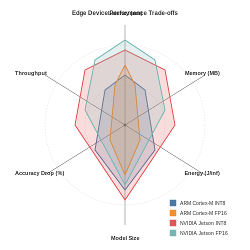
5.2 Benchmarking on Edge Devices
Performance Metrics for Edge Deployment
Benchmarking quantized models on edge devices requires evaluating trade-offs between accuracy, latency, memory footprint, and power consumption. Key metrics include:
- Inference Latency: Measured in milliseconds (ms), this quantifies the time taken for a forward pass on the target hardware.
- Peak Memory Usage: The maximum RAM consumed during inference, critical for devices with limited resources.
- Energy Efficiency: Often measured in joules per inference (J/inf), derived from power profiling tools.
- Model Size: Post-quantization footprint in megabytes (MB), affecting storage and loading times.
Hardware-Specific Optimization Challenges
Edge devices like ARM Cortex-M microcontrollers or NVIDIA Jetson platforms exhibit divergent performance characteristics under quantization:
- Fixed-Point vs. Floating-Point: ARM NEON accelerators handle 8-bit integer (INT8) operations efficiently, while GPUs may retain FP16 support.
- Memory Bandwidth: Quantization reduces DRAM access but may increase cache misses if tensor layouts are suboptimal.
- Compiler Optimizations: Frameworks like TensorFlow Lite for Microcontrollers leverage CMSIS-NN kernels for ARM, while TVM optimizes for RISC-V.
Quantitative Analysis Framework
The effective quantization ratio (EQR) measures the practical speedup accounting for hardware constraints:
where \( T \) denotes latency, \( \Delta_{\text{acc}} \) is the relative accuracy drop, and \( \alpha \) is a device-specific scaling factor (typically 0.2–1.5).
Case Study: MobileNetV3 on Raspberry Pi 4
When deploying a QAT-trained MobileNetV3-Small (224×224 input) at INT8 precision:
- Latency: Reduced from 58ms (FP32) to 14ms (INT8) using TensorRT.
- Memory: Peak usage dropped from 420MB to 110MB.
- Accuracy: Top-1 ImageNet accuracy declined by 1.8% (67.4% → 65.6%).
Profiling Tools and Methodologies
Accurate benchmarking requires:
- Hardware Counters: ARM Streamline or Intel VTune for cycle-level analysis.
- Power Monitors: Nordic Power Profiler Kit for µA-resolution measurements.
- Statistical Rigor: Reporting 95th percentile latency across 10,000 inferences to capture thermal throttling effects.
Energy-Aware Quantization Strategies
For battery-constrained devices, per-layer energy profiling reveals optimization priorities:
where \( E_{\text{comp}} \) scales with MAC operations and \( E_{\text{mem}} \) depends on off-chip accesses. Mixed-precision quantization (e.g., INT8 for convolutions, INT16 for attention) often yields better energy-accuracy Pareto frontiers.
5.3 Comparing with Full-Precision Models
The performance gap between quantized models and their full-precision counterparts stems from several fundamental limitations imposed by reduced numerical precision. When comparing quantized models (typically 8-bit or lower) against full-precision (32-bit floating point) models, three key aspects dominate the analysis: representational capacity, gradient propagation, and accumulated quantization error.
Representational Capacity and Dynamic Range
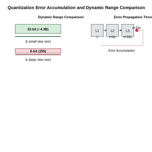
The most immediate difference lies in the dynamic range of representable values. For an n-bit quantization, the number of discrete levels is given by:
For 8-bit quantization (n=8), this yields 255 discrete levels compared to the ~4.3 billion distinct values representable in 32-bit floating point. The reduced dynamic range forces trade-offs between precision for small values and coverage of large values. The quantization function Q for a floating-point value x can be expressed as:
where Δ is the quantization step size (xmax - xmin)/L. This clipping and rounding operation introduces irreversible information loss that compounds through network layers.
Gradient Mismatch in Backpropagation
Quantization-aware training employs straight-through estimators (STE) to approximate gradients through the non-differentiable quantization function. While STE enables gradient flow, it creates a mismatch between the forward and backward passes:
This approximation ignores the staircase nature of the quantization function, leading to suboptimal weight updates compared to full-precision training where gradients are exact.
Error Accumulation Across Layers
The quantization error ε = Q(x) - x propagates through the network in a non-linear fashion. For a deep network with L layers, the final output error δL can be modeled as:
where Ji is the Jacobian of layer i's operations and δ0 is the initial quantization error. The cross-terms between Jacobians and quantization error derivatives cause error accumulation that doesn't exist in full-precision models.
Empirical Performance Characteristics
Practical observations across computer vision and NLP benchmarks reveal consistent patterns:
- Accuracy Drop: 8-bit models typically show 0.5-2% accuracy reduction on ImageNet classification compared to FP32 baselines
- Convergence Speed: Quantized models require 10-30% more training iterations to reach comparable loss values
- Sensitivity to Initialization: Weight initialization becomes more critical as quantization amplifies poor initial conditions
The performance gap widens significantly for lower bit-widths (4-bit and below), where specialized techniques like mixed-precision training or non-uniform quantization become necessary to maintain usable accuracy.
Case Study: Transformer Model Quantization
In large language models, attention mechanisms exhibit particular sensitivity to quantization. The softmax operation in attention layers:
suffers from significant approximation error when xi values are quantized, as the exponential function's non-linearity magnifies small quantization errors. This explains why transformer models often show larger accuracy drops than CNNs when quantized to 8-bit precision.
6. Key Research Papers
6.1 Key Research Papers
- JOURNAL OF LA Towards Accurate Post-training Quantization for ... — This work was supported by National Key Research and Development Program of China (2022YFC3602601), and Key Research and Development ... Wen Fei is with the Department of Electronic Engineering, Shanghai Jiao Tong University, Shanghai 200240, China (e-mail: [email protected]). ... B. Model Quantization Quantization-aware training (QAT) [14 ...
- Frontiers | Ps and Qs: Quantization-Aware Pruning for Efficient Low ... — We study various configurations of pruning during quantization-aware training, ... and focus on related work around the key techniques covered in this paper. Pruning. Early work (LeCun et al., ... This work was performed using the Pacific Research Platform Nautilus HyperCluster supported by NSF awards CNS-1730158, ACI-1540112, ACI-1541349, OAC ...
- Llm-qat: D -free Quantization Aware Training for Language Models — activations. To ensure efficient quantization, we adopt the per-token activation quantization and per-channel weight quantization. For a comprehensive evaluation of the different quantizer choices, we provide the ablation study in Section 3.3.2. Quantization-aware training for key-value cache In addition to weight and activation quantization, 1
- PDF Q-DiT: Accurate Post-Training Quantization for Diffusion Transformers — quantization: Quantization-Aware Training (QAT) [2,5,9] and Post-Training Quantization (PTQ) [21,25]. QAT inte-grates the quantization process directly into the fine-tuning phase, leveraging STE [1] to simultaneously optimize quan-tizer parameters and model parameters during fine-tuning. This approach restores the model's performance degrada-
- Quantune: Post-training quantization of convolutional neural networks ... — Quantization-aware training ... (KAIST), in 2017-2018. His research interests include energy-aware mobile computing and deep learning compiler. ... Yongin Kwon received the B.Sc. degree in electrical and electronic engineering from the Korea Advanced Institute of Science and Technology (KAIST), South Korea, in 2008, and the M.S. and Ph.D ...
- PDF Overcoming Forgetting Catastrophe in Quantization-Aware Training — quantization process, LifeQuant, to overcome the for-getting catastrophe in quantization-aware training. 2. We theoretically analyze the forgetting problem caused by the search space shift with the change of data tasks. Thus, we propose Proximal Quantization Space Search (ProxQ) to regularize the shift during quantization to
- GitHub - facebookresearch/SpinQuant: Code repo for the paper "SpinQuant ... — Code repo for the paper "SpinQuant LLM quantization with learned rotations" - facebookresearch/SpinQuant ... The number of bits for key quantization--w_clip: Whether using the grid search to find best weight clipping range ... Data-Free Quantization Aware Training for Large Language Models . License. BiT is CC-BY-NC 4.0 licensed as of now. ...
- PDF Reducing the Side-Effects of Oscillations in Training of Quantized YOLO ... — Figure 2. Trajectory of activation quantization threshold during training for same toy example as in Fig.1. Even the scale factors for activation quantization oscillate during the optimization. 3. Preliminaries Here we provide a brief background on the quantization-aware training (QAT) and introduce the issue of oscillations in QAT using a ...
- PDF Optimal Clipping and Magnitude-aware Differentiation for Improved ... — Optimal Clipping and Magnitude-aware Differentiation for Improved Quantization-aware Training DoReFa-Net (Zhou et al., 2016) increased the forward preci-sion to 4-bit and used max-scaling, i.e., matching the largest quantized representation to the largest value in the set of elements (tensor or vector) to be quantized.
- JOURNAL OF LA Towards Accurate Post-Training Quantization of Vision ... — This paper presents ERQ, an innovative two-step PTQ method specifically crafted to reduce quantization errors arising from activation and ... Intelligence, School of Informatics, and Key Laboratory of Multimedia Trusted Perception and Efficient Computing, Ministry of Education of China, Xiamen ... is known as quantization-aware training (QAT ...
6.2 Open-Source Implementations
- PDF Data Generation for Hardware-Friendly Post-Training Quantization — deployment [26,42]. While quantization-aware training (QAT) incorporates quantization during the training process to help maintain the original accuracy [11,23], post-training quantization (PTQ) [1,9,16,30,40] has gained significant traction for its ability to compress the model without re-quiring retraining. However, PTQ's effectiveness depends
- PDF Aspects and best practices of quantization aware training for custom ... — 2 The process of quantization aware training In this section, the common approach for quantization aware training is de-scribed, which is followed by many works. The core idea is to mimmic the quantization behavior of the target hardware within a oating point based training scheme. This is done by inserting so called fake quantization nodes
- Deploying YOLOv5 on NVIDIA Jetson Orin with cuDLA: Quantization-Aware ... — Its open-source implementation enables developers to leverage pretrained models and customize them according to specific goals. The following sections walk through an end-to-end YOLOv5 cuDLA sample that shows you how to: Train a YOLOv5 model with Quantization-Aware Training (QAT) and export it for deployment on DLA.
- PDF End-to-end codesign of Hessian-aware quantized neural networks for ... — Quantization-aware training (QAT) has been shown to be very successful in scaling down model sizes for FPGAs [10, 11, 15, 17, 28, 33]. With QAT, large NNs can be quantized to 8 bits and below, with comparable accuracy to the baseline. Quantized NNs (QNNs) generally have considerably reduced model sizes and latencies. Hessian-aware quantization
- Quantization aware approximate multiplier and hardware accelerator for ... — Quantization aware approximate multiplier and hardware accelerator for edge computing of deep learning applications. ... training and inference of deep learning applications are executed on the cloud servers. ... An open-source library of approximate adders and multipliers was released for fast design space generation and exploration ...
- Model quantization techniques — ROCm Documentation — How to fine-tune LLMs with ROCm. bitsandbytes#. The ROCm-aware bitsandbytes library is a lightweight Python wrapper around CUDA custom functions, in particular 8-bit optimizer, matrix multiplication, and 8-bit and 4-bit quantization functions. The library includes quantization primitives for 8-bit and 4-bit operations through bitsandbytes.nn.Linear8bitLt and bitsandbytes.nn.Linear4bit and 8 ...
- AI:Deep Quantized Neural Network support - stm32mcu - STMicroelectronics — 7. Evidence of efficient code generation. Similar to the qkeras.print_qstats() function or the extended summary() function in Larq, the analyze command reports a summary of the number of operations used for each generated C-layer according the type of data. The number of operation types for the entire generated C-model is also reported. This last information makes it possible to know if the ...
6.3 Recommended Books and Tutorials
- Model quantization techniques — ROCm Documentation — How to fine-tune LLMs with ROCm. bitsandbytes#. The ROCm-aware bitsandbytes library is a lightweight Python wrapper around CUDA custom functions, in particular 8-bit optimizer, matrix multiplication, and 8-bit and 4-bit quantization functions. The library includes quantization primitives for 8-bit and 4-bit operations through bitsandbytes.nn.Linear8bitLt and bitsandbytes.nn.Linear4bit and 8 ...
- PDF Hardware-Aware Mixed-Precision Neural Networks using In-Train Quantization — 3. We show that our quantization scheme can be infused with adversarial training, im-proving robustness by 1:4pp and reducing the number of bit operations by 1:9 , when compared to a uniformly quantized ResNet56. 2 Related Work 2.1 Quantization-Aware Training By limiting the weights and activations of CNNs to a constrained set of values, it becomes
- Qualcomm-AI-research/transformer-quantization - GitHub — To combat these challenges, we present three solutions based on post-training quantization and quantization-aware training, each with a different set of compromises for accuracy, model size, and ease of use. In particular, we introduce a novel quantization scheme {--} per-embedding-group quantization.
- PDF 16.36: Communication Systems and Networks Lecture 5 - Quantization - MIT — the quantization values Clearly 1 depends on 2 and vice versa. The two can be solved iteratively to obtain an optimal quantizer. Lloyd-Max algorithm: Start with arbitrary regions (e.g., uniform Δ) A) Find optimal quantization values ("centroids") B) Use quantization values to get new regions ("midpoints")
- QAT: EfficientNet Quantization Aware Training | Quadric — In this tutorial we allow 2 paths: (1) use the PyTorch 2 Export (pt2e) library to perform quantization-aware training (QAT) on EfficientNet-B7, and export it such that it can be run through ONNX Runtime and (2) export a pre-trained QAT model from PyTorch so that it can be lowered in CGC. Notes:
- Training Quantized Neural Networks with ADMM Approach — quantization using ADMM. DQ is the abbreviation of Dynamic Quan-tization. QAT is the abbreviation of Quantization aware training. ..44 6.4 Table of the accuracies on dataset Pendigits in the case of 8 bits, 4 bits, 2 bits, 1 bit. PTQ is the abbreviation of Post training quan-tization. QNN-STE is the abbreviation of training quantized neural
- Quantization Process - an overview | ScienceDirect Topics — The general quantization methods can be classified into: static vs. dynamic, uniform vs. mixed precision, Post Training Quantization (PTQ) vs. Quantization-aware Training (QAT). Table 5 provides high-level definitions of these different methods and serves as a background for the rest of the transformer-specific methods.
- Sub 8-Bit Quantization of Streaming Keyword Spotting Models for ... — We propose a novel 2-stage sub 8-bit quantization aware training algorithm for all components of a 250K parameter feedforward, streaming, state-free keyword spotting model. ... Download book PDF. Download book EPUB. Text, Speech, and ... Electronics (2021) Google Scholar Vanhoucke, V., Senior, A., Mao, M.Z.: Improving the speed of neural ...