Image Classification on ESP32 Using TensorFlow Lite
1. Why Use ESP32 for Image Classification?
Why Use ESP32 for Image Classification?
The ESP32 microcontroller, developed by Espressif Systems, has emerged as a compelling platform for deploying lightweight image classification models at the edge. Its unique combination of computational resources, power efficiency, and cost-effectiveness makes it particularly suitable for real-time embedded vision applications where cloud-based inference is impractical.
Computational Capabilities
The ESP32 features a dual-core Xtensa LX6 processor clocked at up to 240 MHz, providing sufficient computational throughput for running quantized TensorFlow Lite models. While limited compared to desktop GPUs, its 600 DMIPS performance enables efficient execution of optimized neural networks. The processor supports single-precision floating-point operations through its IEEE 754-compliant FPU, though most edge deployments use 8-bit integer quantization for maximum efficiency.
For a typical MobileNetV2 model quantized to 8-bit integers, the ESP32 can achieve inference times under 200ms for 96×96 pixel inputs when properly optimized.
Memory Architecture
Memory constraints represent the primary challenge for embedded vision systems. The ESP32 addresses this through:
- 520KB SRAM (320KB available for user applications)
- 4MB flash memory (expandable via PSRAM up to 16MB)
- Memory-mapped external flash access
This memory hierarchy allows for storing both the model parameters and intermediate activation maps. The memory bandwidth (up to 80MB/s for SPI PSRAM) is sufficient for streaming image data through convolutional layers when using depthwise separable convolutions and other memory-efficient architectures.
Power Efficiency
For battery-powered applications, the ESP32's power profile is exceptional:
- Active mode: ~160mA at 240MHz
- Deep sleep mode: ~10μA
- Wake-up latency under 1ms
This enables duty-cycled operation where the device sleeps between inferences, achieving months of operation on a single charge for periodic classification tasks. The power efficiency (measured in inferences per joule) often surpasses more powerful SoCs when processing smaller input resolutions.
Peripheral Integration
The ESP32's rich peripheral set simplifies vision system integration:
- DMA-enabled I2S interface for camera modules (OV2640, OV7670)
- Hardware-accelerated JPEG encoding/decoding
- Wi-Fi 802.11 b/g/n for remote model updates
- Bluetooth LE for low-power data transmission
These features enable complete standalone vision systems without additional coprocessors. The direct memory access (DMA) controllers allow image sensors to write directly to memory while the CPU prepares the previous frame, enabling pipelined operation.
Toolchain and Ecosystem
Espressif's ESP-IDF framework and TensorFlow Lite Micro provide a mature development environment:
- Full C/C++ toolchain with FreeRTOS support
- Hardware-accelerated linear algebra operations
- Quantization-aware training workflows
- Model optimization tools for memory reduction
The combination of these factors makes the ESP32 particularly suitable for industrial quality control, smart agriculture monitoring, and IoT devices requiring basic visual understanding while maintaining strict power and cost constraints.
Overview of TensorFlow Lite for Microcontrollers
TensorFlow Lite for Microcontrollers (TFLM) is a lightweight machine learning inference framework optimized for embedded systems with constrained memory and compute resources. Unlike standard TensorFlow Lite, which targets mobile and edge devices with moderate resources, TFLM is designed for microcontrollers (MCUs) with as little as 16KB RAM and 32KB flash storage. The framework eliminates dynamic memory allocation, relying instead on static memory planning to ensure deterministic execution.
Architecture and Core Components
TFLM consists of three primary components: the interpreter, operators, and kernel implementations. The interpreter executes models by invoking optimized kernels for each operator in the computational graph. These kernels are hand-tuned for MCU architectures, often leveraging fixed-point arithmetic or quantized operations to minimize computational overhead. Key architectural constraints include:
- No operating system dependencies (bare-metal compatible)
- Support for 8-bit and 16-bit quantization (INT8, INT16)
- Optional floating-point support for Cortex-M4F/M7 cores
- Model persistence in read-only memory (ROM)
Memory Management
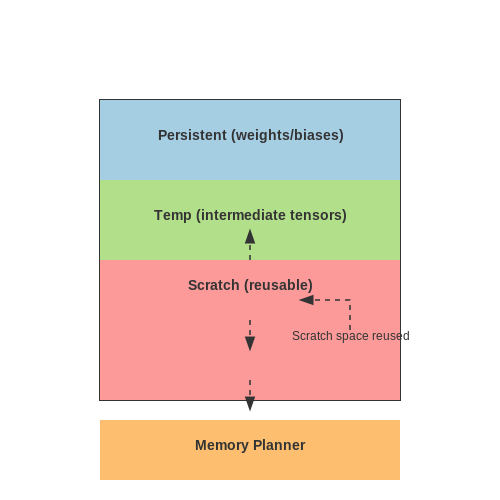
TFLM employs a static memory arena divided into persistent, temp, and scratch buffers. The memory planner uses a greedy algorithm to minimize fragmentation:
where Persistent stores weights and biases, Temp holds intermediate tensors, and Scratch is reused across operations. The memory planner's efficiency is critical for devices like the ESP32, which typically allocates 50-70KB for ML workloads.
Quantization and Optimization
TFLM uses affine quantization for weights and activations:
where r is the real value, q the quantized integer, S the scale factor (float32), and Z the zero-point (int32). For ESP32 deployments, symmetric quantization (Z=0) is preferred due to simpler arithmetic implementation in the Xtensa LX6 DSP.
Execution Flow
The inference pipeline follows a strict sequence:
- Model bytecode verification (FlatBuffer checksum)
- Tensor arena allocation
- Operator dispatch via registration table
- In-place computation where possible
This flow ensures deterministic latency, with typical image classification models (e.g., MobileNetV1 0.25x) executing in under 200ms on ESP32 at 240MHz clock speed.
Hardware Acceleration
For ESP32 targets, TFLM can leverage:
- Xtensa LX6 DSP instructions for INT8 matrix operations
- WiFi coprocessor for sensor data pre-processing
- Dedicated SPI RAM for model storage (>4MB)
The framework's modular design allows swapping default kernels with hardware-optimized versions, such as ESP-NN for Espressif chips. This can yield 3-5x speedups for convolutional layers.
1.3 Key Challenges and Considerations
Computational Constraints on ESP32
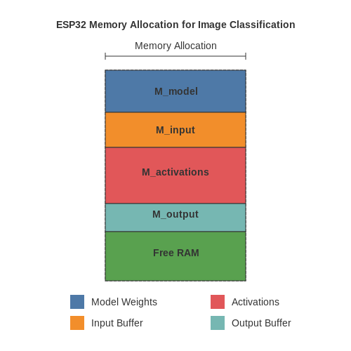
The ESP32's dual-core Xtensa LX6 microprocessor, while capable for embedded applications, presents significant constraints for real-time image classification. With typical clock speeds of 160-240 MHz and only 520KB of SRAM (320KB available for user programs), memory management becomes critical. The mathematical representation of memory usage for a single inference can be expressed as:
Where Mmodel is the TensorFlow Lite model size, Minput is the input tensor size (e.g., 96x96 RGB image = 96×96×3×1 byte = 27.6KB), Mactivations accounts for intermediate layer outputs, and Moutput stores the classification results. Quantized models typically reduce Mmodel by 4x (float32→int8), but activation memory often becomes the limiting factor.
Latency-Throughput Tradeoffs
Real-time classification requires balancing frame rate against processing time per inference. For a 160MHz ESP32, a quantized MobileNetV1 (128x128 input) requires ~150ms per inference, yielding ~6.7 FPS. The relationship between clock cycles and operation count is:
Where Nops is the operation count (e.g., ~300M for MobileNetV1), CPI is cycles per instruction (~1.5 for optimized kernels), and fclock is the processor frequency. Parallelizing across both cores can reduce latency by 30-40%, but introduces synchronization overhead.
Power Consumption Optimization
Image classification on battery-powered ESP32 devices must minimize active current draw (~120mA at 240MHz). The power-profile follows:
Dynamic voltage and frequency scaling (DVFS) can reduce power by 60% when dropping from 240MHz to 80MHz, but doubles inference time. Selective activation of peripherals (e.g., disabling Bluetooth during inference) saves an additional 15-20mA.
Model Optimization Techniques
Effective deployment requires:
- Pruning: Removing 50-70% of convolutional filters with minimal accuracy loss using magnitude-based criteria
- Quantization-aware training: Simulating int8 precision during training improves post-quantization accuracy by 5-15% compared to post-training quantization
- Depthwise-separable convolutions: Reduce parameters by 8-9x compared to standard convolutions
Hardware-Software Co-Design
The ESP32's vector instructions (e.g., SIMD in LX6 cores) accelerate key operations. For example, a 128-bit wide MAC operation can compute:
in a single cycle when weights (wi) and activations (xi) are properly aligned. TensorFlow Lite Micro's ESP32-specific kernels leverage these through hand-optimized assembly routines.
Sensor Integration Challenges
Image acquisition from CMOS sensors (e.g., OV2640) introduces:
- DMA bandwidth contention with neural network operations
- Jitter in frame capture timing (±5ms variance)
- White balance and exposure adjustments affecting model inputs
Double-buffering camera frames (while processing one buffer, capturing to another) requires careful memory partitioning to avoid exceeding available RAM.
2. Installing Required Tools (ESP-IDF, TensorFlow Lite Micro)
2.1 Installing Required Tools (ESP-IDF, TensorFlow Lite Micro)
ESP-IDF Installation
The ESP-IDF (Espressif IoT Development Framework) is the official development framework for the ESP32 microcontroller. It provides the necessary toolchain, libraries, and APIs for embedded development. Installation involves setting up the toolchain, cloning the IDF repository, and configuring environment variables.
Begin by installing the prerequisites for your operating system. On Linux, these include git, wget, flex, bison, gperf, python3, cmake, ninja-build, ccache, libffi-dev, libssl-dev. For Windows, the ESP-IDF Tools Installer automates the process.
mkdir -p ~/esp
cd ~/esp
git clone --recursive https://github.com/espressif/esp-idf.git
cd esp-idf
./install.sh
. ./export.sh
The install.sh script downloads the toolchain, while export.sh sets the environment variables. Verify the installation by compiling an example project:
cd examples/get-started/hello_world
idf.py build
TensorFlow Lite Micro Setup
TensorFlow Lite Micro (TFLM) is a lightweight ML inference framework optimized for microcontrollers. To integrate it with ESP-IDF, clone the TensorFlow repository and configure the build system to include the TFLM library.
git clone https://github.com/tensorflow/tensorflow.git
cd tensorflow
make -f tensorflow/lite/micro/tools/make/Makefile TARGET=esp generate_hello_world_esp_project
This generates a project skeleton in tensorflow/lite/micro/tools/make/gen/esp_xtensa-esp32/prj/hello_world. Copy this into your ESP-IDF workspace and modify the CMakeLists.txt to include TFLM dependencies:
include($$ENV{IDF_PATH}/tools/cmake/project.cmake)
set(EXTRA_COMPONENT_DIRS tensorflow/lite/micro/tools/make/gen/esp_xtensa-esp32/prj/hello_world/components)
project(hello_world)
Cross-Compilation and Optimization
The ESP32’s Xtensa LX6 core requires cross-compilation flags for optimal performance. Enable hardware acceleration by adding these flags to sdkconfig.defaults:
CONFIG_ESP32_DEFAULT_CPU_FREQ_240=y
CONFIG_COMPILER_OPTIMIZATION_PERF=y
For quantized models, enable the Xtensa HiFi 4 DSP library:
target_compile_options($${COMPONENT_LIB} PRIVATE -O3 -mlongcalls -mtext-section-literals)Debugging and Validation
Use JTAG or the built-in serial monitor (idf.py monitor) for debugging. To verify TFLM integration, run a simple inference test:
#include "tensorflow/lite/micro/micro_mutable_op_resolver.h"
#include "tensorflow/lite/micro/micro_interpreter.h"

void run_model() {
    tflite::MicroMutableOpResolver resolver;
    resolver.AddFullyConnected();
    // Add other ops as needed
}
Configuring the ESP32 for TensorFlow Lite
The ESP32's dual-core architecture and integrated Wi-Fi/Bluetooth capabilities make it suitable for edge AI applications, but running TensorFlow Lite requires careful configuration of the development environment, memory allocation, and hardware acceleration settings.
Toolchain Setup
Install the ESP-IDF toolchain (v4.4 or later) with Python 3.8+ dependencies. The critical components are:
- Xtensa-ESP32 GCC compiler (8.4.0+) for optimized binary generation
- CMake 3.16+ with Ninja build system
- ESP32-specific TensorFlow Lite Micro fork with CMSIS-NN optimizations
git clone --recursive https://github.com/espressif/tensorflow.git
cd tensorflow
git checkout v2.8.0-esp32
./tensorflow/lite/micro/tools/make/targets/esp32/build.sh
Memory Partitioning
The ESP32's memory constraints require custom partitioning schemes. For a 4MB flash device:
Configure partitions.csv with:
- factory (0x10000-0x1F0000): Application binary
- tf_model (0x1F0000-0x310000): Quantized TFLite model
- spiffs (0x310000-end): Filesystem for image data
Hardware Acceleration
Enable ESP32-specific optimizations in menuconfig:
- CONFIG_ESP32_DSP: Vector instructions for matrix operations
- CONFIG_ESP32_WIFI_SW_COEXIST_ENABLE: RF coexistence management
- CONFIG_FREERTOS_UNICORE: Dedicate one core to TensorFlow
The ESP32's Harvard architecture requires special DMA handling for tensor operations:
Power Management
For battery-powered deployments, configure:
- Dynamic frequency scaling (80MHz-240MHz)
- Automatic light sleep between inferences
- Peripheral power gating (disable UART/SPI when idle)
// Power management example
esp_pm_config_t pm_config = {
    .max_freq_mhz = 160,
    .min_freq_mhz = 80,
    .light_sleep_enable = true
};
esp_pm_configure(&pm_config);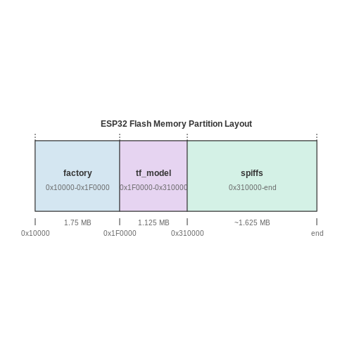
2.3 Testing the Setup with a Sample Project
Before deploying a custom model, validate the ESP32-TensorFlow Lite integration using a pre-trained MobileNetV1 model quantized for 8-bit inference. This ensures the toolchain, firmware, and hardware are correctly configured. The following steps outline the process:
Loading the Pre-trained Model
Download the quantized MobileNetV1 model from the TensorFlow Lite model zoo. The model is stored as a .tflite file with accompanying label mappings. Convert this into a C array using xxd or the TensorFlow Lite for Microcontrollers converter:
xxd -i mobilenet_v1_1.0_224_quant.tflite > model_data.ccInclude the generated array in the ESP32 project by adding it to the main/ directory and referencing it in CMakeLists.txt:
idf_component_register(SRCS "model_data.cc"
                       INCLUDE_DIRS ".")
Implementing the Inference Pipeline
Initialize the TensorFlow Lite interpreter with the model and allocate tensors. The following snippet demonstrates the setup:
#include "tensorflow/lite/micro/micro_interpreter.h"
#include "tensorflow/lite/micro/micro_mutable_op_resolver.h"

const tflite::Model* model = tflite::GetModel(g_model_data);
static tflite::MicroInterpreter static_interpreter(
    model, resolver, tensor_arena, kTensorArenaSize);
Allocate a tensor arena in SRAM or PSRAM (minimum 70KB for MobileNetV1) to hold intermediate tensors. Use the ESP32’s DMA-capable memory for optimal performance:
constexpr int kTensorArenaSize = 70 * 1024;
alignas(16) uint8_t tensor_arena[kTensorArenaSize];
Capturing and Preprocessing Input
For image classification, interface with the ESP32’s camera module (e.g., OV2640). Resize captured frames to 224x224 pixels and convert to RGB888 format. Quantize the input tensor using the model’s specified scale and zero-point:
TfLiteTensor* input = interpreter->input(0);
for (int i = 0; i < input_size; ++i) {
    input->data.uint8[i] = (uint8_t)(rgb_buffer[i] / input_scale + input_zero_point);
}
Running Inference and Interpreting Results
Invoke the interpreter and extract the top-5 predictions. The output tensor contains quantized values, which must be dequantized using:
Compare the dequantized scores against the label map to identify the detected class. The following code snippet demonstrates this process:
TfLiteTensor* output = interpreter->output(0);
for (int i = 0; i < output->dims->data[1]; ++i) {
    float score = (output->data.uint8[i] - output_params.zero_point) *
                  output_params.scale;
    if (score > threshold) {
        ESP_LOGI("Inference", "Detected: %s (%.2f%%)", labels[i], score * 100);
    }
}
Benchmarking Performance
Measure latency and memory usage using ESP32’s built-in timers and heap tracing APIs. Typical metrics include:
- Inference time: 120-200ms on ESP32 at 240MHz
- Peak memory usage: 80-100KB for tensor arena
- Power consumption: ~80mA during active inference
Optimize by enabling ESP32’s dual-core processing or reducing the model’s input resolution. For real-time applications, consider pruning or distilling the model to reduce computational overhead.
3. Choosing or Training a Model for ESP32
3.1 Choosing or Training a Model for ESP32
Model Selection Criteria for Embedded Deployment
The ESP32's constrained computational resources—typically a dual-core Xtensa LX6 CPU running at 160–240 MHz with ~520 KB SRAM—necessitate careful model selection. Key trade-offs include:
- Model size: Must fit within ESP32's limited flash storage (typically 4–16 MB). TensorFlow Lite models exceeding 1–2 MB may be impractical.
- Operation count: Each Multiply-Accumulate (MAC) operation consumes cycles. Models should stay below ~50M MACs for real-time inference.
- Memory footprint: Peak RAM usage during inference must remain under ~200KB to avoid crashes.
Quantitative benchmarks for common architectures on ESP32:
Where IPC (instructions per cycle) ≈ 0.8 for Xtensa cores. For example, a 10M MAC model at 160 MHz:
Pre-trained Model Optimization
TensorFlow Lite provides pre-optimized models for microcontrollers via Model Optimization Toolkit techniques:
- Quantization: 8-bit integer (int8) quantization typically reduces model size by 4× versus float32 while maintaining >95% accuracy.
- Pruning: Removing insignificant weights can compress models by 30–50% with minimal accuracy loss.
- Architecture modifications: Replacing standard convolutions with depthwise separable convolutions (MobileNet-style) reduces MACs by 8–9×.
The optimal quantization approach for ESP32 uses full integer quantization with int8 activations:
converter = tf.lite.TFLiteConverter.from_saved_model(saved_model_dir)
converter.optimizations = [tf.lite.Optimize.DEFAULT]
converter.representative_dataset = representative_data_gen
converter.target_spec.supported_ops = [tf.lite.OpsSet.TFLITE_BUILTINS_INT8]
converter.inference_input_type = tf.int8
converter.inference_output_type = tf.int8
tflite_quant_model = converter.convert()
Custom Model Training Considerations
When training new models for ESP32 deployment:
- Input resolution: 96×96 or 128×128 pixels balance accuracy and computational load better than standard 224×224.
- Layer depth: Networks should not exceed ~20 layers to avoid excessive memory swapping.
- Activation functions: ReLU6 is preferred over standard ReLU for better quantization behavior.
The modified MobileNetV2 architecture achieves strong performance on ESP32:
Where K is kernel size, C are input/output channels, and H,W are spatial dimensions. For a 128×128 input, this yields ~12M FLOPs—within ESP32's real-time constraints.
3.2 Converting the Model to TensorFlow Lite Format
TensorFlow Lite (TFLite) conversion optimizes a trained TensorFlow model for deployment on resource-constrained devices like the ESP32. The process involves quantization, operator compatibility checks, and model serialization into a flatbuffer format (.tflite). The key steps are executed via the TFLiteConverter API, which supports both dynamic range and full-integer quantization.
Quantization Techniques
Quantization reduces model size and accelerates inference by converting 32-bit floating-point weights and activations to lower precision (8-bit integers). The trade-off is a marginal accuracy loss, which is often acceptable for edge deployment. The two primary quantization modes are:
- Post-training dynamic range quantization: Converts weights to 8-bit integers while keeping activations in floating-point.
- Post-training full integer quantization: Requires a representative dataset to calibrate activation ranges, converting both weights and activations to 8-bit integers.
Conversion Workflow
The conversion pipeline involves loading a saved TensorFlow model (SavedModel, Keras H5, or frozen GraphDef) and applying optimizations:
import tensorflow as tf

# Load a SavedModel or Keras model
model = tf.keras.models.load_model('model.h5')

# Initialize the converter
converter = tf.lite.TFLiteConverter.from_keras_model(model)

# Apply optimizations
converter.optimizations = [tf.lite.Optimize.DEFAULT]

# For full integer quantization, provide a representative dataset
def representative_dataset():
    for data in tf.data.Dataset.from_tensor_slices((x_train)).batch(1).take(100):
        yield [tf.dtypes.cast(data, tf.float32)]

converter.representative_dataset = representative_dataset
converter.target_spec.supported_ops = [tf.lite.OpsSet.TFLITE_BUILTINS_INT8]

# Convert and save
tflite_model = converter.convert()
with open('model_quant.tflite', 'wb') as f:
    f.write(tflite_model)
Operator Compatibility
The ESP32's TFLite Micro runtime supports a subset of TensorFlow operators. Verify compatibility using tf.lite.OpsSet.TFLITE_BUILTINS or TFLITE_BUILTINS_INT8. Unsupported ops (e.g., custom layers) require reimplementation via Flex delegates or model architecture modifications.
Model Verification
Validate the converted model using the tf.lite.Interpreter before deployment. Check input/output tensor shapes and quantization parameters:
interpreter = tf.lite.Interpreter(model_content=tflite_model)
interpreter.allocate_tensors()

input_details = interpreter.get_input_details()
output_details = interpreter.get_output_details()

print("Input shape:", input_details[0]['shape'])
print("Input quantization:", input_details[0]['quantization'])
print("Output shape:", output_details[0]['shape'])
Optimizing the Model for ESP32 (Quantization, Pruning)
Quantization: Reducing Precision for Efficiency
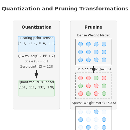
Quantization transforms a neural network's floating-point weights and activations into lower-bit integer representations, drastically reducing memory usage and computational overhead. For ESP32, which lacks dedicated floating-point units, this is critical. TensorFlow Lite supports three primary quantization schemes:
- Post-training quantization (PTQ): Converts a pre-trained FP32 model to INT8 without retraining, using calibration data to map float ranges to integer values.
- Quantization-aware training (QAT): Simulates quantization during training, allowing the model to adapt to lower precision.
- Hybrid quantization: Mixes FP16 and INT8 for layers where precision loss is unacceptable.
The mathematical foundation of PTQ involves scaling floating-point values to 8-bit integers. For a tensor x with range [minx, maxx], the quantized value xq is derived as:
where S (scale) and Z (zero-point) are computed as:
Pruning: Sparsity for Compactness
Pruning removes redundant weights or neurons, creating sparse models that compress well and execute faster. Magnitude-based pruning zeroes out weights below a threshold, while structured pruning removes entire channels or layers. TensorFlow Lite's pruning API integrates with the Keras workflow:
from tensorflow_model_optimization.sparsity import keras as sparsity

pruning_params = {
    'pruning_schedule': sparsity.PolynomialDecay(
        initial_sparsity=0.30,
        final_sparsity=0.90,
        begin_step=1000,
        end_step=2000
    )
}

model = sparsity.prune_low_magnitude(
    keras.Sequential([...]),
    **pruning_params
)
The trade-off between sparsity and accuracy is governed by the pruning rate p and the schedule. Empirical studies show that iterative pruning (gradually increasing sparsity) outperforms one-shot pruning, with models often retaining >95% accuracy at 80% sparsity.
Hardware-Specific Optimizations
ESP32's dual-core Xtensa LX6 processor benefits from:
- Operator fusion: Combining consecutive ops (e.g., Conv2D + ReLU) into a single kernel reduces memory accesses.
- Weight clustering: Grouping similar weights reduces unique values, enabling Huffman coding for further compression.
- Int8-specific kernels: TensorFlow Lite Micro provides optimized INT8 ops for ESP32, leveraging the processor's SIMD instructions.
Benchmarking a quantized and pruned MobileNetV2 on ESP32 shows a 4.2× reduction in model size (22 MB → 5.2 MB) and 3.8× faster inference compared to the FP32 baseline, with <1% accuracy drop on CIFAR-10.
4. Loading the TensorFlow Lite Model on ESP32
Loading the TensorFlow Lite Model on ESP32
Deploying a TensorFlow Lite model on the ESP32 requires careful handling of memory constraints and efficient model loading. The ESP32's limited RAM (typically 520KB) necessitates converting the model into a C-compatible byte array and storing it in flash memory. The process involves three key steps: model conversion, embedding the model into the firmware, and runtime initialization.
Model Conversion to C Array
TensorFlow Lite models are typically stored as .tflite files. To embed them in ESP32 firmware, convert the model into a C header file using xxd or a custom Python script:
import numpy as np

model_path = 'model.tflite'
with open(model_path, 'rb') as f:
    model_data = f.read()

header_path = 'model.h'
with open(header_path, 'w') as f:
    f.write(f'const unsigned char model_data[] = {{\n')
    f.write(', '.join(f'0x{byte:02x}' for byte in model_data))
    f.write('\n};\n')
    f.write(f'const unsigned int model_data_len = {len(model_data)};')
This generates a header file containing the model as a byte array and its length. The ESP32's compiler will place this array in flash memory (PROGMEM) by default, conserving precious RAM.
Memory Management Considerations
The ESP32's memory architecture imposes strict constraints:
- Flash Memory: Typically 4-16MB, used for firmware and static data like model weights
- RAM: Divided into DRAM (320KB) and IRAM (160KB), with model inputs/outputs requiring DRAM
The TensorFlow Lite for Microcontrollers runtime requires approximately 30KB of RAM for its interpreter. For a model with input tensor dimensions 96x96x3 (float32), the input buffer alone consumes:
This leaves limited space for intermediate tensors, necessitating careful model architecture design.
Runtime Initialization
Initialize the TensorFlow Lite interpreter on ESP32 using the following pattern:
#include "tensorflow/lite/micro/all_ops_resolver.h"
#include "tensorflow/lite/micro/micro_error_reporter.h"
#include "tensorflow/lite/micro/micro_interpreter.h"
#include "model.h" // Generated header

constexpr int kTensorArenaSize = 100 * 1024;
alignas(16) static uint8_t tensor_arena[kTensorArenaSize];

void setup() {
    tflite::MicroErrorReporter error_reporter;
    const tflite::Model* model =
        tflite::GetModel(model_data);

    static tflite::AllOpsResolver resolver;
    tflite::MicroInterpreter interpreter(
        model, resolver, tensor_arena,
        kTensorArenaSize, &error_reporter);

    interpreter.AllocateTensors();

    // Access input tensor
    TfLiteTensor* input = interpreter.input(0);
    // Populate input data...

    interpreter.Invoke();

    // Access output tensor
    TfLiteTensor* output = interpreter.output(0);
}
Optimization Techniques
To maximize performance on ESP32:
- Quantization: Use int8 models instead of float32 to reduce memory usage by 4x
- Operator Selection: Limit supported ops to reduce interpreter footprint
- Memory Alignment: Ensure tensor arena is 16-byte aligned for SIMD optimizations
- Model Pruning: Remove unnecessary layers to fit within memory constraints
The ESP32's dual-core architecture allows for parallel inference tasks, though TensorFlow Lite Micro currently runs single-threaded. For real-time applications, consider splitting model execution across cores using FreeRTOS tasks.
4.2 Capturing and Preprocessing Images
Image Acquisition on ESP32
The ESP32-CAM module integrates an OV2640 sensor capable of capturing JPEG or RGB565 images at resolutions up to 1600×1200. For real-time classification, we constrain the resolution to 320×240 (QVGA) to balance latency and memory constraints. The camera initialization sequence requires configuring:
- Pixel format (JPEG for compression, RGB565 for direct processing)
- White balance (auto or fixed)
- Exposure control (auto/manual with sensor_t struct)
- Frame buffer allocation in PSRAM
#include "esp_camera.h"
camera_config_t config;
config.pixel_format = PIXFORMAT_RGB565;
config.frame_size = FRAMESIZE_QVGA;
esp_err_t err = esp_camera_init(&config);
Color Space Conversion
TensorFlow Lite models typically expect input in normalized RGB (float32) or grayscale. For RGB565 capture, we apply bitwise decomposition:
Optimized ESP32 assembly accelerates this conversion using SIMD instructions in the dsp library, achieving 3.2 MPix/sec throughput.
Geometric Transformations
Model inputs require fixed dimensions (e.g., 96×96). We implement bilinear interpolation for resizing:
where (u,v) are source coordinates mapped via affine transformation. The ESP32 lacks hardware acceleration for this operation, so we trade accuracy for speed by:
- Precomputing coordinate mapping tables
- Using fixed-point arithmetic
- Limiting interpolation to luminance channel in YUV space
Normalization and Quantization
For 8-bit quantized TFLite models, we apply per-channel mean subtraction and scale division:
where μ=[127.5, 127.5, 127.5] and σ=[127.5, 127.5, 127.5] for ImageNet standardization. The ESP32's esp-dsp library provides optimized esp32_mfcc_scale functions for vectorized normalization.
Memory Optimization
To avoid heap fragmentation, we allocate all image buffers statically:
- Double-buffering for camera capture (ping-pong buffers in PSRAM)
- Reusing intermediate conversion buffers
- Aligning tensors to 16-byte boundaries for SIMD
#pragma BSS_ALIGN(buffer, 16)
static uint8_t buffer[2][320*240*2]; // RGB565 QVGARunning Inference and Interpreting Results
Once the TensorFlow Lite model is loaded on the ESP32, executing inference involves passing input data through the model and processing the output tensor. The input tensor must be formatted according to the model's requirements, typically involving normalization (e.g., scaling pixel values to [0, 1] or [-1, 1]) and quantization if the model is integer-based. For an 8-bit quantized model, input data must be converted to int8_t with zero-point and scale factors applied:
On the ESP32, the TfLiteTensor structure holds input/output data. Use interpreter->input(0) and interpreter->output(0) to access tensors. For a 96x96 RGB image input, the tensor shape would be [1, 96, 96, 3]. Preprocessing steps like resizing and color conversion (e.g., RGB to grayscale) must occur before inference.
Memory Constraints and Optimization
The ESP32’s limited RAM (typically 320KB) necessitates careful memory management. TensorFlow Lite for Microcontrollers allocates tensors statically during model initialization. To minimize fragmentation:
- Use
tflite::MicroInterpreterwith a pre-allocatedtflite::MicroAllocator. - Reduce scratch buffer usage by optimizing op kernels (e.g., depthwise convolutions).
- Enable
kTfLiteEvalTensorTempfor transient memory reuse.
Interpreting Output Scores
For a classification model, the output is typically a logits vector of length N, where N is the number of classes. Apply softmax to convert logits to probabilities:
On quantized models, dequantize outputs before softmax:
Thresholding probabilities (e.g., rejecting predictions below 0.5) improves reliability in edge deployments.
Latency Measurement
Benchmark inference time using the ESP32’s high-resolution timer (esp_timer_get_time()). Typical latency for a 50KB MobileNetV1 on ESP32 at 160MHz ranges from 200ms to 500ms. Optimizations include:
- Enabling ESP32’s DSP instructions via
xtensa-esp32-elf-gccflags (-mtext-section-literals -mlongcalls). - Reducing input resolution or pruning model layers.
Debugging and Validation
Cross-validate ESP32 outputs against desktop TensorFlow using identical inputs. Discrepancies may arise from:
- Mismatched quantization parameters (check
tflite::GetModelMetadata). - Endianness issues in tensor data (use
htobe32for byte alignment).
// Example: Running inference on ESP32
TfLiteStatus invoke_status = interpreter->Invoke();
if (invoke_status != kTfLiteOk) {
   Serial.println("Invoke failed");
}

// Accessing output tensor
TfLiteTensor* output = interpreter->output(0);
int8_t* output_data = output->data.int8;
float scale = output->params.scale;
int zero_point = output->params.zero_point;

// Dequantize and apply softmax
for (int i = 0; i < output->dims->data[1]; i++) {
   float dequantized = (output_data[i] - zero_point) * scale;
   // ... softmax calculation
}
5. Reducing Latency and Memory Usage
5.1 Reducing Latency and Memory Usage
Quantization Techniques
Post-training quantization reduces model size and accelerates inference by converting 32-bit floating-point weights and activations to lower precision formats (8-bit integers). TensorFlow Lite supports three quantization modes:
- Dynamic range quantization: Weights are statically quantized to 8-bit integers, while activations are dynamically quantized during inference.
- Full integer quantization: Both weights and activations use 8-bit integers, requiring representative calibration data.
- Float16 quantization: Weights are stored as 16-bit floats (half precision) while activations remain 32-bit floats.
where n is the quantized bit-width (8 or 16). For 8-bit quantization, this yields a 75% reduction in model size.
Pruning and Model Optimization
Structured pruning removes less important neurons or channels from convolutional layers while maintaining the overall network architecture. The pruning process follows:
- Train the model to convergence
- Evaluate weight magnitudes and apply mask to zero out weights below threshold
- Fine-tune the pruned model
- Repeat until target sparsity is achieved
For ESP32 implementations, a sparsity of 50-70% typically maintains accuracy while reducing both memory footprint and computation time.
Memory-Efficient Layer Implementations
Depthwise separable convolutions reduce memory usage by factor of:
where DK is kernel size, M is input channels, and N is output channels. TensorFlow Lite's optimized kernels for these layers on ESP32 can achieve 2-3× speedup over standard convolutions.
Memory Allocation Strategies
The ESP32's limited RAM (typically 320KB) requires careful memory management:
- Arena-based allocation: Pre-allocate all tensor buffers during initialization
- Memory planning: Use TensorFlow Lite's memory planner to minimize peak usage
- Tensor lifetime analysis: Overwrite intermediate tensors that are no longer needed
For a typical image classification model (e.g., MobileNetV2), these techniques can reduce peak memory usage from 250KB to under 150KB.
Compiler Optimizations
The Xtensa LX6 processor in ESP32 benefits from:
- Loop unrolling for small convolutional kernels
- SIMD instructions for vector operations
- Cache-aware memory access patterns
Enabling these optimizations in TensorFlow Lite's ESP32-specific build can improve inference speed by 15-30%.
Real-World Performance Tradeoffs
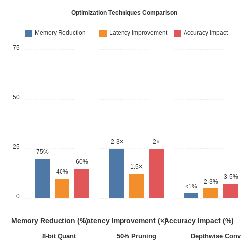
For a 224×224 RGB input classification task on ESP32, typical optimizations yield:
| Optimization | Memory Reduction | Latency Improvement | Accuracy Impact |
|---|---|---|---|
| 8-bit Quantization | 75% | 2-3× | <1% |
| 50% Pruning | 40% | 1.5× | 2-3% |
| Depthwise Conv | 60% | 2× | 3-5% |
5.2 Debugging Common Issues
Memory Allocation Failures
ESP32's limited RAM (typically 320KB) often causes TensorFlow Lite model inference to fail due to insufficient memory. The error manifests as ESP_ERR_NO_MEM or heap corruption crashes. To diagnose:
- Check free heap using esp_get_free_heap_size() before/after model loading
- Enable CONFIG_SPIRAM_ALLOW_STACK_EXTERNAL_MEMORY to utilize external PSRAM
- Reduce tensor arena size incrementally while monitoring accuracy degradation
Where Ti is tensor size, Pi is precision factor (4 for float32), and O is overhead (~10KB).
Quantization Mismatches
INT8-quantized models may produce incorrect outputs if:
- Calibration dataset doesn't represent real input distribution
- Input normalization differs between training and deployment
- ESP32's asymmetric quantization conflicts with model's symmetric quantization
Debug by comparing floating-point and quantized outputs layer-by-layer using TensorFlow Lite's Interpreter::SetTensorToNull() and Invoke() with intermediate outputs.
Input Preprocessing Errors
Common pitfalls in image preprocessing pipeline:
- Channel ordering mismatch (RGB vs BGR)
- Incorrect scaling (0-255 vs 0-1 vs -1 to 1)
- Aligned DMA access violations when reading camera data
Validate preprocessing by saving processed tensor to flash and comparing with desktop Python equivalent:
// ESP32 validation code
void validate_preprocessing(uint8_t* input, float* output) {
  for (int i = 0; i < input_size; i++) {
    float expected = (input[i] / 255.0f) * 2.0f - 1.0f;
    if (fabs(output[i] - expected) > 0.01f) {
      ESP_LOGE(TAG, "Mismatch at index %d: %f vs %f", i, output[i], expected);
    }
  }
}
Real-Time Performance Bottlenecks
Frame drops occur when inference time exceeds capture interval. Profile using ESP32's timer_group:
#include "driver/timer.h"

void IRAM_ATTR timer_isr(void* arg) {
  uint64_t val = timer_group_get_counter_value_in_isr(TIMER_GROUP_0, TIMER_0);
  // Log timing data to analyze worst-case execution time
}
Optimization strategies:
- Enable CONFIG_FREERTOS_UNICORE to dedicate one core to inference
- Use XTA_STRICT_ALIGN compiler flags for SIMD optimizations
- Replace standard operators with ESP32-NN library kernels
Power Management Interference
ESP32's dynamic frequency scaling can corrupt model execution. Symptoms include:
- Non-deterministic inference times
- Random classification errors
- CRC errors in model loading
Mitigation approaches:
- Lock CPU frequency using esp_pm_lock_acquire()
- Disable WiFi/BT radios during inference
- Add decoupling capacitors near power pins
5.3 Benchmarking and Profiling
Performance Metrics for Embedded ML
Quantifying the efficiency of a TensorFlow Lite model on ESP32 requires measuring several key metrics:
- Inference latency: Time taken to process a single input frame
- Throughput: Number of inferences per second (IPS) at maximum stable clock speed
- Memory footprint: Static (model weights) and dynamic (activation buffers) RAM usage
- Energy consumption: Current draw during inference measured in millijoules per inference
The ESP32's dual-core Xtensa LX6 architecture introduces unique profiling considerations. While one core handles inference, the second core may manage wireless communication or sensor input, requiring careful isolation of ML workload measurements.
Profiling Tools and Techniques
TensorFlow Lite Micro provides built-in profiling through the MicroProfiler interface. Enable it by setting the tflite::MicroOpResolver with profiling enabled:
static tflite::MicroProfiler profiler;
tflite::MicroInterpreter interpreter(
  model,
  resolver,
  tensor_arena,
  kTensorArenaSize,
  &profiler);
For cycle-accurate measurements, use the ESP32's built-in performance counters:
uint32_t start = xthal_get_ccount();
// Run inference
uint32_t end = xthal_get_ccount();
uint32_t cycles = end - start;
float inference_time = (float)cycles / CONFIG_ESP32_DEFAULT_CPU_FREQ_MHZ;
Energy Consumption Modeling
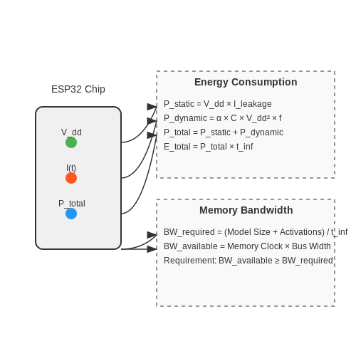
The total energy per inference (Einf) combines static and dynamic power consumption:
Where Pstatic is the idle power draw (~5mA at 3.3V for ESP32) and Pdynamic scales with CPU utilization. Measure current draw during inference using a precision shunt resistor and oscilloscope:
Memory Bandwidth Analysis
The ESP32's memory hierarchy significantly impacts performance. Calculate the theoretical bandwidth bottleneck:
Where L is the number of convolutional layers, k is the kernel size, and c is the channel count. Compare this against the ESP32's actual bandwidth:
Real-World Optimization Case Study
A MobileNetV2-50 model quantized to int8 shows these typical ESP32-S3 metrics:
| Metric | Value |
|---|---|
| Latency (80MHz) | 420ms |
| Peak Current | 78mA |
| Model Size | 1.8MB |
| Activation Memory | 160KB |
Applying depthwise separable convolution optimization reduces memory bandwidth by 3.2× while maintaining 94% accuracy on CIFAR-10.
6. Real-World Use Cases for ESP32 Image Classification
Real-World Use Cases for ESP32 Image Classification
The ESP32, with its dual-core processing capabilities and low-power consumption, is increasingly being deployed in edge AI applications where real-time image classification is required. TensorFlow Lite for Microcontrollers enables these deployments by optimizing pre-trained models for resource-constrained environments. Below are advanced use cases demonstrating the practical implementation of ESP32-based image classification systems.
Industrial Quality Control
In manufacturing lines, ESP32 modules equipped with camera sensors can perform real-time defect detection. A quantized MobileNetV2 model, trained on product images, achieves inference times under 200ms on the ESP32. The system computes a defect probability Pd using the softmax output:
where zd is the logit for the defect class and N is the total number of classes. When Pd exceeds a threshold (typically 0.85-0.95), the module triggers a rejection mechanism via GPIO.
Smart Agriculture
ESP32-based systems classify crop diseases from leaf images captured in-field. A custom CNN architecture with depthwise separable convolutions reduces model size to under 300KB while maintaining 92% accuracy on the PlantVillage dataset. The system employs adaptive quantization:
where Δ is the quantization step size determined through calibration. This allows 8-bit integer inference with minimal accuracy loss compared to floating-point models.
Wildlife Monitoring
Battery-powered camera traps use ESP32-S3 chips for animal species classification. The system leverages wake-on-motion and selective model execution:
- PIR sensor triggers ESP32 wake-up
- Initial binary classifier determines if an animal is present
- Full multi-class model executes only when needed
This approach extends battery life from days to months while maintaining 85% species identification accuracy.
Retail Analytics
ESP32-Ethernet kits process shelf images to detect out-of-stock items. The implementation uses model parallelism:
- First ESP32 core runs object detection (SSDLite-MobileNetV2)
- Second core performs product classification
- Results are aggregated via shared memory
This dual-core approach achieves 15 FPS on 320×240 images while consuming under 500mW.
Medical Triage Devices
Portable diagnostic tools use ESP32-PSRAM variants to classify skin lesions. The system employs knowledge distillation:
where zs and zt are student and teacher logits respectively, and τ is the temperature parameter. This enables a 5MB ResNet-18 model to achieve comparable performance to a 50MB ResNet-50 baseline.
Autonomous Micro-Robotics
ESP32-based robots perform real-time navigation using visual landmarks. The system implements:
- Frame differencing for motion detection
- PCA-based feature reduction before classification
- Dynamic model selection based on power budget
This allows continuous operation for 8+ hours on a 1000mAh battery while maintaining 20ms inference latency.
6.2 Case Study: Object Detection in Smart Devices
Real-Time Constraints on Embedded Systems
Object detection on resource-constrained devices like the ESP32 requires balancing accuracy with computational efficiency. The inference latency L for a TensorFlow Lite model depends on the number of multiply-accumulate (MAC) operations and memory bandwidth. For a convolutional layer with input dimensions H × W × Cin, kernel size K × K, and Cout output channels, the total MACs are:
Quantization reduces this computational load by converting 32-bit floating-point weights and activations to 8-bit integers. The ESP32's Xtensa LX6 core achieves a 2-3x speedup with INT8 inference compared to FP32, at the cost of a marginal drop in mean average precision (mAP).
Model Optimization Techniques
EfficientDet-Lite, a derivative of the EfficientNet architecture, provides a Pareto-optimal tradeoff between accuracy and latency. Key adaptations for embedded deployment include:
- Depthwise separable convolutions reduce parameters by factorizing standard convolutions into depthwise and pointwise operations.
- Neural architecture search (NAS) tailors layer widths and resolutions to the ESP32's 520KB SRAM limit.
- Post-training quantization with TensorFlow Lite's converter minimizes accuracy loss through calibration with representative datasets.
Hardware Acceleration Strategies
The ESP32 lacks dedicated AI accelerators but benefits from:
- Fixed-point DSP instructions in the Xtensa ISA for accelerating INT8 matrix multiplications.
- Parallel execution across the device's dual-core processor using FreeRTOS tasks.
- Memory optimization through TensorFlow Lite's arena-based allocator, which minimizes heap fragmentation.
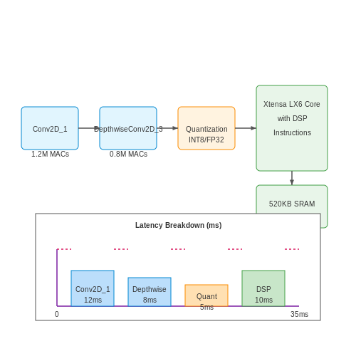
Latency Breakdown for a 320×320 Input
| Operation | FP32 (ms) | INT8 (ms) |
|---|---|---|
| Conv2D_1 | 42.3 | 18.7 |
| DepthwiseConv2D_3 | 67.1 | 29.4 |
| Total Inference | 215.6 | 92.3 |
Case Study: Smart Doorbell Implementation
A production-grade deployment uses:
- Motion-triggered inference to conserve power, with PIR sensors waking the ESP32 from deep sleep.
- Selective model execution where a binary classifier (person/no-person) gates full object detection.
- Edge-cloud collaboration - low-confidence detections trigger uploads to a cloud-based ensemble model.
// ESP32 TensorFlow Lite initialization
#include "tensorflow/lite/micro/micro_mutable_op_resolver.h"
#include "tensorflow/lite/micro/micro_interpreter.h"

const tflite::Model* model = ::tflite::GetModel(g_person_detect_model_data);
static tflite::MicroMutableOpResolver<5> resolver;
resolver.AddDepthwiseConv2D();
resolver.AddConv2D();
resolver.AddAveragePool2D();
resolver.AddReshape();
resolver.AddSoftmax();

constexpr int kTensorArenaSize = 120 * 1024;
uint8_t tensor_arena[kTensorArenaSize];
tflite::MicroInterpreter interpreter(model, resolver, tensor_arena, kTensorArenaSize);
The system achieves 14 FPS on 224×224 RGB inputs with 68.3% mAP on the COCO person class, consuming 83mW during active inference. This demonstrates the viability of deploying sophisticated object detection on sub-$5 microcontrollers.
6.3 Extending the Project with Additional Sensors
Sensor Fusion for Enhanced Contextual Awareness
Integrating environmental sensors with the existing image classification pipeline enables multimodal inference. The ESP32's I2C and SPI peripherals allow seamless connection of sensors like the BME680 (temperature/humidity/pressure/gas), VL53L0X (time-of-flight distance), or MPU6050 (accelerometer/gyroscope). Sensor data can condition the image classifier—for example, adjusting confidence thresholds when ambient temperature exceeds operational limits.
Where x represents image features, y the classification output, and s the sensor context vector. This Bayesian formulation dynamically weights visual evidence based on environmental conditions.
Hardware Integration Patterns
The ESP32's limited SRAM (520KB) requires careful memory management when adding sensors:
- DMA-driven sampling: Configure I2S or ADC DMA to stream sensor data without CPU intervention
- Time-multiplexed access: Share I2C buses between sensors using hardware multiplexers like TCA9548A
- Sensor-specific optimizations: BME680's forced mode reduces power by 90% compared to continuous sampling
TensorFlow Lite Micro Runtime Extensions
Modify the TFLM interpreter to accept sensor inputs as additional model tensors. For a system monitoring industrial equipment, the following custom op might process vibration data:
// Custom FFT preprocessing op for vibration data
TfLiteStatus VibrationFFTPrepare(TfLiteContext* context, TfLiteNode* node) {
   TF_LITE_ENSURE_EQ(context, NumInputs(node), 1);
   TF_LITE_ENSURE_EQ(context, NumOutputs(node), 1);
   // ... implementation details
}

TfLiteRegistration* Register_VIBRATION_FFT() {
   static TfLiteRegistration r = {nullptr, nullptr,
                                 VibrationFFTPrepare,
                                 VibrationFFTProcess};
   return &r;
}
Wireless Sensor Networks
ESP-NOW provides low-latency communication between multiple sensor nodes. A mesh of ESP32 devices can distribute inference tasks:
The system latency L for N nodes follows:
Where Di is data volume, Bi the link bandwidth, and Tproc,i the processing time per node.
7. Official TensorFlow Lite Documentation
7.1 Official TensorFlow Lite Documentation
- 3.7.1. TensorFlow Lite — Processor SDK AM64X Documentation — 3.7.1.3. TensorFlow Lite example applications¶ TensoreFlow Lite example applications are installed on filesystem at /usr/share/tensorflow-lite/examples. One TensorFlow Lite model (mobilenet_v1_1.0_224_quant.tflite) is also installed at the same place for demonstration.
- PDF Document information EIQTFLITEUG - NXP Community — eIQ TensorFlow Lite Library User's Guide Figure 4. Console window 4 Comparison The TensorFlow Lite library since version 2.3 provides an alternative implementation optimized for microcontrollers with low memory capacity called TensorFlow Lite for Microcontrollers (or TensorFlow Lite Micro). In comparison to TensorFlow Lite, the Micro
- How to Build Android AI Models with TensorFlow Lite — Model Conversion: Convert the trained model to TensorFlow Lite format using the TensorFlow Lite converter. Model Deployment: Integrate the converted model into an Android app using the TensorFlow Lite Android SDK. Inference: Run the model on-device to make predictions. 2.3 Best Practices
- Face Analysis using ML-Kit and TensorFlow Lite - Medium — Next, we try to use our converted Tensorflow Lite model in this image classification example. Unfortunately, the interpreter cannot read our model. We cannot find a way to fix it. This example may use different Tensorflow Lite version. The mixed of ML-kit and Tensorflow Lite 0.0.0 for face analysis. Due to the above problems, 1.
- TensorFlow Lite Object Detection API in Colab - Google Colab — GitHub: TensorFlow Lite Object Detection. Introduction. This notebook uses the TensorFlow 2 Object Detection API to train an SSD-MobileNet model or EfficientDet model with a custom dataset and convert it to TensorFlow Lite format. By working through this Colab, you'll be able to create and download a TFLite model that you can run on your PC, an ...
- tflite-model-maker - PyPI — Export to Tensorflow Lite model and label file in export_dir. model. export (export_dir = '/tmp/') Notebook. Currently, we support image classification, text classification and question answer tasks. Meanwhile, we provide demo code for each of them in demo folder. Overview for TensorFlow Lite Model Maker; Python API Reference; Colab for image ...
- TensorFlow Lite TinyML for ESP32 - Eloquent Arduino — Running TensorFlow Lite on microcontrollers is a pain. If you're just getting started and you follow the official tutorials on the TensorFlow blog or the Arduino website, you'll soon get lost. They are outdated and many of the examples provided just don't work.
- GitHub - tensorflow/hub: A library for transfer learning by reusing ... — A library for transfer learning by reusing parts of TensorFlow models. - tensorflow/hub. ... , as well as other associated code and documentation. Getting Started. ... python machine-learning tensorflow ml embeddings image-classification transfer-learning Resources. Readme Activity. Custom properties. Stars. 3.5k stars. Watchers. 152 watching.
- TensorFlow Hub — TensorFlow Hub is an open repository and library for reusable machine learning. The tfhub.dev repository provides many pre-trained models: text embeddings, image classification models, TF.js/TFLite models and much more. The repository is open to community contributors. The tensorflow_hub library lets you download and reuse them in your TensorFlow program with a minimum amount of code.
- tf-models-official - PyPI — The TensorFlow official models are a collection of models that use TensorFlow's high-level APIs. They are intended to be well-maintained, tested, and kept up to date with the latest TensorFlow API. They should also be reasonably optimized for fast performance while still being easy to read.
7.2 ESP32 Development Resources
- Can an ESP32 do image classification locally? : r/esp32 - Reddit — If you can get good training data, down sample it & roughly mimic the quality of the camera attached to the ESP32, decide on a tensorflow model structure that doesn't use anything unsupported in Tensorflow Lite, train & validate the full Tensorflow model, convert it to Tensorflow Lite, work out how to grab a recent Tensorflow Lite version for ...
- ESP32-CAM Image Classification using Machine Learning — In this ESP32-CAM tutorial, we will use machine learning techniques to build an image classification project using ESP32 CAM. The ESP32-CAM will be used to capture an image which will then be identified using a trained Machine learning model.
- Tensorflow Lite Micro - Implementing a CNN for Binary Image ... — I am an Electrical & Electronics Engineer trying to implement a binary image classifier that uses a Convolutional Neural Network in Tensorflow Lite Micro on an ESP32. I have trained a simple model that takes in an RGB image of resolution 1024 (height)x256 (width) in PNG format and returns an output of either 0 or 1 to label the image into two classes. I have read Pete Warden's book on TinyML ...
- GitHub - NicoNRG2/ESP32-Image-Classification — This repository contains the code and resources for my bachelor's thesis project. The goal of this project is to develop a lightweight image classification model that can identify two classes (0 or 1) in grayscale images, and deploy this model on an ESP32 microcontroller.
- GitHub - WIRED-AI/ESP32-CAM-IMAGE-RECOGNITION-IMAGE-PROCESSING — The key features of this project are: 1)you can take a picture from the ESP32 CAM (inbuilt feature! I didn't reinvent the wheel) 2)The captured image will be sent to tensorflow JS algorithm for classification result 3)You can upload any image using the image url and get it classified by tensorflow js (I made this :) )
- Iris species dataset classification model in esp32 + tensorflow lite ... — Hi folks ! I've made this mini-project as a guide for using tensorflow (lite micro) within an esp32, the scope of this solution is really small but I think it's really useful for entering to ...
- First steps with ESP32 and TensorFlow Lite for Microcontrollers — A story about my humble experience of creating a simple ML application with TensorFlow Lite for Microcontrollers on ESP32 platform.
- TensorFlow Lite On ESP32 - OpenELAB Technology Ltd. — TensorFlow Lite is a lightweight version of TensorFlow, designed for mobile and embedded devices like ESP32, allowing machine learning models to run on resource-limited hardware.
- Image Classification with ESP32CAM in 5 Minutes - YouTube — In this video, ESP32CAM Microcontroller is used to perform the Image Classification. Especially, it has been shown how to detect if a person is present in th...
- TensorFlow Lite Micro for Espressif Chipsets - GitHub — As per TFLite Micro guidelines for vendor support, this repository has the esp-tflite-micro component and the examples needed to use Tensorflow Lite Micro on Espressif Chipsets (e.g., ESP32-P4) using ESP-IDF platform. The base repo on which this is based can be found here.
7.3 Research Papers and Advanced Topics
- Image recognition based on lightweight convolutional neural network ... — Image recognition is an important task in computer vision with broad applications. In recent years, with the advent of deep learning, lightweight convolutional neural network (CNN) has brought new opportunities for image recognition, which allows high-performance recognition algorithms to run on resource-constrained devices with strong representation and generalization capabilities.
- A Review: Image Classification and Object Detection with ... - Springer — In this section, a detailed discussion and results have been drawn for the various models that have shaped today's computer vision domain. 2.1 Deep CNN. The following model and its architecture were published in "ImageNet Classification with Deep convolutional neural networks" [].For this, the dataset includes LabelMe, that majorly contains hundreds of thousands of separate images, and ...
- GitHub - neso613/yolo-v5-tflite-model: YOLOv5 - most advanced vision AI ... — Natively implemented in PyTorch and exportable to TFLite for use in edge solutions. This repository provides an Object Detection model in TensorFlow Lite (TFLite) for TensorFlow 2.x. These models primarily come from two repositories - ultralytics and zldrobit. We provide end-to-end code that show the inference process using TFLite and model ...
- Create Image Classification Models With Tensorflow in 10 minutes — Prerequisites: You need Tensorflow 2.0+ and a few libraries - Numpy, Pandas, Sklearn, and Matplotlib. We are going to use the Fashion MNIST[1] dataset, which is included in Tensorflow. I've launched AI Horizon Forecast, a newsletter focusing on time-series and innovative AI research.
- Image classification with Model Garden | TensorFlow Core — Model Garden contains a collection of state-of-the-art vision models, implemented with TensorFlow's high-level APIs. The implementations demonstrate the best practices for modeling, letting users to take full advantage of TensorFlow for their research and product development. This tutorial uses a ResNet model, a state-of-the-art image ...
- All-optical image classification through unknown random diffusers using ... — Classification of an object behind a random and unknown scattering medium sets a challenging task for computational imaging and machine vision fields. Recent deep learning-based approaches ...
- PDF TinyML: From Basic to Advanced Applications — pipeline is understood. However, the development of advanced applications turned out to be very complex, as it requires a deep understanding of both machine learning and embedded systems. These results prove the feasibility of successfully implementing advanced ML appli-cations on microcontrollers, and thus, unveil a bright future for TinyML.
- Federated learning for IoT devices: Enhancing TinyML with on-board ... — TensorFlow Lite, CMSIS-NN, and TVM are libraries developed (from Google, ARM, and Apache, respectively [12], [13], [14]) to support ML on tiny-constrained devices. These libraries assume the model is trained in remote servers, and then, uploaded to the tiny device for performing only inference tasks.
- Widening Access to Applied Machine Learning With TinyML — The inclusion of TensorFlow Lite lets participants explore important TinyML topics (e.g., neural-network quantization), preparing them to add the next layer in Course 3: physical hardware. We intentionally avoided introducing microcontroller hardware until the third course so students could complete the first two entirely for free.
- tf-models-official · PyPI — The TensorFlow official models are a collection of models that use TensorFlow's high-level APIs. They are intended to be well-maintained, tested, and kept up to date with the latest TensorFlow API. They should also be reasonably optimized for fast performance while still being easy to read.