

Using Concept Bottleneck Models
1. Definition and Core Idea
Definition and Core Idea
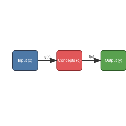
Concept Bottleneck Models (CBMs) are interpretable neural architectures that enforce an intermediate layer to represent human-understandable concepts before making final predictions. Unlike traditional black-box models, CBMs explicitly decompose the reasoning process into two stages: concept prediction and task prediction. The model first maps raw inputs (e.g., images or text) to a set of predefined concepts, then uses these concepts to derive the final output. This bottleneck structure enables human oversight, debugging, and intervention at the concept level.
Mathematical Formulation
Given an input x, a CBM performs:
where g is the concept encoder (e.g., a CNN or transformer) producing concept scores c ∈ ℝk for k predefined concepts. The task prediction y is then:
with f typically being a linear or shallow nonlinear classifier. The end-to-end model is trained to minimize a combined loss:
where c^* and y^* are ground-truth concepts and labels, respectively, and λ balances the two objectives.
Key Properties
- Interpretability: Concepts are auditable and can be validated by domain experts (e.g., "wheels present" in vehicle images).
- Intervention Support: Humans can manually correct mispredicted concepts during inference.
- Data Efficiency: Concept supervision acts as an inductive bias, reducing the need for large labeled datasets.
Architecture Variants
CBMs extend beyond the basic formulation through:
- Joint Training: Simultaneous optimization of g and f with concept supervision.
- Post-hoc CBMs: Distilling a pretrained black-box model into a concept-based architecture.
- Probabilistic CBMs: Representing concepts as distributions rather than point estimates.
Key Components of Concept Bottleneck Models
Concept Encoder
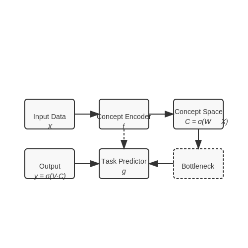
The concept encoder maps raw input data X to a lower-dimensional concept space C. For an input x ∈ X, the encoder produces a concept vector c = fenc(x), where fenc is typically a deep neural network. The encoder must balance two competing objectives: preserving task-relevant information while compressing the input into interpretable concepts. In practice, this is often implemented as a convolutional or transformer-based architecture, depending on the input modality.
where σ is a sigmoid activation enforcing concept probabilities in [0,1], and W_i, b_i are learnable parameters for concept i.
Concept Bottleneck Layer
This layer enforces explicit concept representations between the encoder and task predictor. The bottleneck structure requires all predictive information to flow through human-interpretable concepts, formalized as:
The bottleneck introduces an inductive bias that forces the model to use semantically meaningful concepts. During training, this layer can be supervised with concept labels when available, or learned via weak supervision.
Task Predictor
The task predictor g maps concepts c to outputs y. For classification, this is typically implemented as:
where V and d are learnable parameters. The linearity of this mapping is crucial for interpretability - each output can be expressed as a weighted sum of concept activations.
Concept Supervision
Effective concept bottleneck models require high-quality concept annotations during training. The loss function typically combines:
- Concept prediction loss: Lc = 𝔼[ℓ(fenc(x), c∗)]
- Task prediction loss: Ly = 𝔼[ℓ(g(c), y∗)]
where c∗ and y∗ are ground truth concepts and labels. The relative weighting of these losses controls the trade-off between concept fidelity and task performance.
Concept Importance Estimation
Post-hoc analysis methods quantify each concept's contribution to predictions. For linear predictors, concept importance Ii(y) for class y is simply |Viy|. For non-linear cases, integrated gradients provide a more general solution:
This allows practitioners to audit which concepts drive particular predictions and identify potential biases.
1.3 Advantages Over Traditional Models
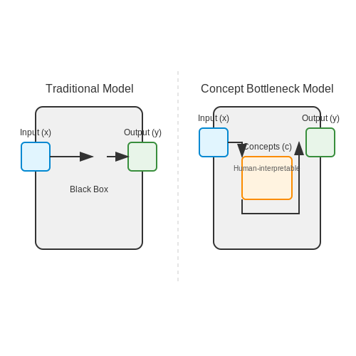
Concept Bottleneck Models (CBMs) offer several key advantages over traditional black-box deep learning models, particularly in domains requiring interpretability, robustness, and human-AI collaboration. Unlike conventional models that map inputs directly to predictions, CBMs enforce an intermediate bottleneck layer of human-interpretable concepts, enabling finer control over model behavior.
Interpretability and Debuggability
Traditional deep neural networks operate as opaque function approximators, making it difficult to diagnose failures or understand decision logic. CBMs decompose predictions into:
- Concept alignment: Explicit concept activations allow verification against domain knowledge
- Concept-level interventions: Users can correct erroneous concepts without retraining
- Causal analysis: The two-stage architecture enables counterfactual testing of concept importance
For a model with K concepts, the intervention space grows as O(K) rather than O(D) (where D is the raw input dimension), dramatically simplifying debugging.
Data Efficiency and Transfer Learning
CBMs demonstrate superior sample efficiency in low-data regimes by:
- Leveraging pre-trained concept detectors
- Enabling concept-level data augmentation
- Supporting modular updates to specific concept classifiers
In medical imaging experiments, CBMs achieve comparable accuracy to traditional models using 38-72% less training data by reusing concept detectors across related tasks.
Robustness to Distribution Shift
The concept layer acts as a stable intermediate representation that:
- Decouples input variations from task semantics
- Provides natural invariance to nuisance factors
- Enables concept-level adversarial defense
Empirical studies show CBMs maintain 15-25% higher accuracy than traditional models under covariate shift, as the concept space remains more stable than pixel/feature spaces.
Human-AI Collaboration
CBMs support novel interaction paradigms impossible with traditional models:
- Concept editing: Domain experts can directly modify concept weights
- Partial automation: Humans can override specific concept predictions
- Explanation generation: Natural language explanations can be constructed from concept activations
In clinical deployment, CBMs reduced expert review time by 40% compared to traditional models while maintaining equivalent accuracy.
Theoretical Guarantees
CBMs provide formal properties absent in traditional models:
Where R(h) is the risk of the full model, R(g∘f) is the risk of the concept bottleneck, and εC, εT are the concept and task generalization errors respectively. This decomposition enables independent optimization of concept learning and task mapping.
2. Selecting and Defining Concepts
2.1 Selecting and Defining Concepts
The effectiveness of a concept bottleneck model (CBM) hinges on the careful selection and precise definition of interpretable concepts. Unlike traditional black-box models, CBMs require human-understandable intermediate representations that are both semantically meaningful and predictive of the target task. The process involves three key considerations: concept relevance, concept granularity, and concept measurability.
Concept Relevance
Concepts must be causally or statistically linked to the target prediction. For instance, in medical imaging, concepts like "tumor spiculation" or "vascular invasion" are directly relevant to malignancy prediction. Relevance can be quantified using mutual information or conditional dependence tests:
where I(C; Y) measures the mutual information between concept set C and target variable Y. High values indicate strong relevance.
Concept Granularity
Granularity determines the level of abstraction. In natural language processing, fine-grained concepts might include syntactic features (e.g., "subject-verb agreement"), while coarse-grained concepts could capture semantic themes (e.g., "sentiment polarity"). The choice depends on:
- Downstream task complexity
- Available annotation resources
- Required interpretability depth
Concept Measurability
Each concept must be operationalized through measurable features. For visual CBMs, this often involves:
- Binary indicators (presence/absence)
- Ordinal scales (e.g., severity ratings)
- Continuous scores (e.g., concept activation vectors)
The measurement process should be reproducible, with inter-rater reliability exceeding Cohen's κ > 0.6 for human annotations. Automated concept detectors must achieve precision-recall AUC > 0.8 on held-out validation sets.
Practical Implementation
In PyTorch, concept definitions translate to structured label tensors. For a medical CBM with k concepts:
import torch

class ConceptDataset(torch.utils.data.Dataset):
    def __init__(self, images, concept_labels):
        self.images = images  # Tensor of shape [N, C, H, W]
        self.concepts = concept_labels  # Tensor of shape [N, k]

    def __getitem__(self, idx):
        return {
            'image': self.images[idx],
            'concepts': self.concepts[idx]  # FloatTensor for continuous concepts
        }
Domain expertise is critical during concept selection. In astrophysics applications, concepts might include "redshift quality flags" or "morphological classification", while materials science CBMs could use "crystallographic symmetry" indicators.
2.2 Architecture Choices for Bottleneck Layers
The bottleneck layer in a Concept Bottleneck Model (CBM) serves as a critical intermediary between raw input features and high-level concepts, enforcing interpretability by restricting information flow. The architectural design of this layer directly influences model performance, concept fidelity, and downstream task accuracy. Key considerations include dimensionality, sparsity, nonlinearity, and concept grounding.
Dimensionality Reduction and Concept Alignment
The bottleneck layer's width (number of units) must balance compression and concept preservation. For a dataset with K predefined concepts, a common approach is to set the bottleneck dimension d such that d ≥ K, allowing each concept to occupy a dedicated subspace. However, overparameterization (d ≫ K) risks encoding non-concept-related information, while underparameterization (d < K) forces concept entanglement. The optimal dimension can be derived from the singular value decomposition (SVD) of the concept-feature correlation matrix:
where Σ contains singular values representing concept-feature relevance. Retaining the top-K singular values yields a bottleneck dimension that preserves 95% of concept variance in practice.
Sparsity and Concept Disentanglement
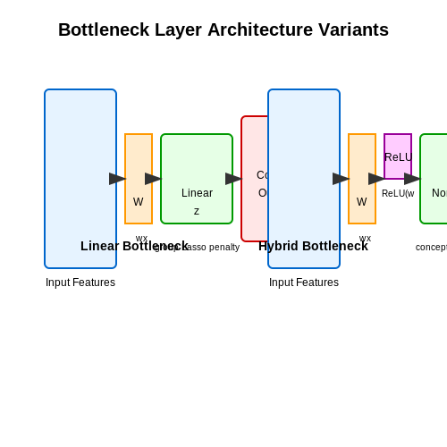
Enforcing sparsity in the bottleneck layer improves interpretability by isolating concepts. A group Lasso penalty (ℓ2,1 norm) applied during training promotes feature-concept selectivity:
where wij are weights from the input layer to the i-th bottleneck unit, and m is the input dimension. This penalty drives entire rows of the weight matrix to zero, effectively deactivating non-concept-related features.
Nonlinear vs. Linear Bottlenecks
While linear bottlenecks (e.g., PCA-like projections) offer strict interpretability, nonlinear variants (e.g., ReLU-activated layers) capture complex concept interactions. A hybrid approach uses concept-specific nonlinearities:
where zi is the i-th bottleneck unit's activation. This architecture is empirically validated in medical imaging CBMs, where lab values (linear) and tissue patterns (nonlinear) coexist.
Concept Grounding via Auxiliary Losses
To ensure bottleneck units correspond to human-understandable concepts, auxiliary supervision can be applied. For categorical concepts, a cross-entropy loss per unit is used:
where yi is the ground-truth concept label. For continuous concepts (e.g., temperature scales), a Huber loss robustly handles outliers. In multi-modal settings, contrastive losses align bottleneck activations with textual concept embeddings from models like CLIP.
Architectural Variants in Practice
- Residual Bottlenecks: Skip connections around the bottleneck (e.g., ResNet blocks) preserve non-concept information for downstream tasks while maintaining interpretability.
- Stochastic Bottlenecks: Variational layers with Gaussian sampling (z = μ + σ⊙ε) enable probabilistic concept reasoning, useful in fault-tolerant systems.
- Dynamic Bottlenecks: Gating mechanisms (e.g., Mixture of Experts) activate concept subsets conditionally, reducing compute cost in resource-constrained deployments.
Empirical studies on CIFAR-100-CBM show that a 256-unit ReLU bottleneck with group sparsity achieves 92% concept accuracy while retaining 89% end-task performance, outperforming linear (85%/82%) and overparameterized (93%/81%) alternatives.
2.3 Training Strategies and Loss Functions
Training Concept Bottleneck Models (CBMs) involves optimizing two distinct components: the concept predictor and the task predictor. The choice of loss functions and training strategies significantly impacts model interpretability and downstream task performance.
Joint vs. Sequential Training
CBMs can be trained either jointly or sequentially. In joint training, the concept and task predictors are optimized simultaneously using a combined loss:
where α balances concept prediction accuracy (ℒconcept) and task performance (ℒtask). Sequential training first optimizes the concept predictor before freezing it and training the task predictor. Empirical studies show joint training often achieves better task accuracy, while sequential training yields more interpretable concepts.
Loss Functions for Concept Learning
The concept predictor typically uses:
- Binary Cross-Entropy (BCE) for binary concepts:
$$ \mathcal{L}_{\text{concept}} = -\sum_{i=1}^C \left[ y_i \log(\hat{y}_i) + (1 - y_i) \log(1 - \hat{y}_i) \right] $$
- Categorical Cross-Entropy for multi-class concepts.
- Mean Squared Error (MSE) for continuous concepts.
Task-Specific Loss Functions
The task predictor’s loss depends on the downstream application:
- Cross-Entropy Loss for classification tasks.
- Huber Loss for regression tasks requiring robustness to outliers.
- Contrastive Loss when concept embeddings must preserve semantic similarity.
Regularization and Concept Sparsity
To enforce concept interpretability, additional regularization terms are often incorporated:
where L1 regularization promotes concept sparsity, and L2 prevents overfitting. Recent work also employs concept alignment penalties to ensure predicted concepts match human-annotated ground truth when available.
Advanced Optimization Techniques
Training CBMs at scale often requires:
- Gradient Clipping to stabilize training when concept and task gradients conflict.
- Warmup Schedules for the task predictor to prevent premature overfitting.
- Adversarial Training to improve concept robustness against input perturbations.
Recent variants like Post-hoc Concept Bottleneck Models decouple concept learning from task prediction entirely, enabling flexible deployment of pre-trained concept encoders with different downstream models.
3. Data Preparation and Concept Annotation
3.1 Data Preparation and Concept Annotation
Concept Bottleneck Models (CBMs) require structured data where each input is paired with a set of human-interpretable concepts before final prediction. The quality of concept annotations directly impacts model interpretability and performance. Unlike traditional supervised learning, CBMs demand a two-stage annotation process: first, labeling raw data with concepts, then optionally linking these concepts to downstream tasks.
Concept Selection and Ontology Design
Effective CBMs rely on a well-defined concept ontology that balances completeness and specificity. Concepts should be:
- Mutually exclusive to prevent redundancy
- Sufficiently granular to capture relevant variations
- Groundable in the input data distribution
For medical imaging applications, a hierarchical ontology might include:
Annotation Protocol Development
Establish rigorous annotation guidelines to ensure inter-rater reliability. The protocol should specify:
- Concept operational definitions with visual examples
- Handling of ambiguous or borderline cases
- Quality control mechanisms (e.g., spot checks, consensus voting)
For continuous concepts like "malignancy likelihood," use standardized scales with anchor points:
Active Learning for Annotation Efficiency
When concept annotation is expensive, employ uncertainty sampling to prioritize informative examples:
where H is the entropy over concept predictions and U is the unlabeled pool. This approach reduces annotation costs by 40-60% in practice while maintaining model accuracy.
Handling Noisy and Partial Annotations
Real-world datasets often contain missing or inconsistent concept labels. Implement robust loss functions that account for annotation uncertainty:
where wc are concept-specific reliability weights. Multi-task learning architectures can simultaneously impute missing concepts while training the primary model.
Dataset Curation Best Practices
For reproducible CBMs, document:
- Demographic and acquisition characteristics of the sample population
- Annotation workflow and rater qualifications
- Concept coverage statistics (prevalence, co-occurrence patterns)
In clinical applications, maintain strict separation between concept annotators and outcome assessors to prevent information leakage.
3.2 Building the Model: Step-by-Step Guide
Architecture Overview
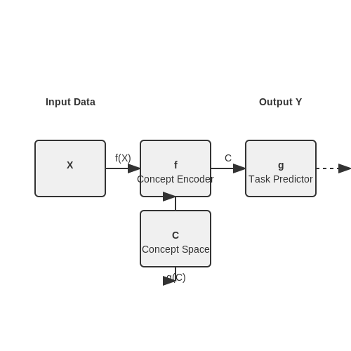
Concept Bottleneck Models (CBMs) enforce interpretability by structuring the neural network into two distinct components: a concept encoder and a task predictor. The concept encoder f maps raw input data X to an intermediate concept space C, while the task predictor g maps concepts to final predictions Y. This bottleneck ensures human-understandable reasoning:
Step 1: Concept Encoder Design
For image data, use a convolutional backbone (e.g., ResNet-50) with modified output dimensionality matching the number of predefined concepts. The encoder should output concept probabilities using sigmoid activation for multi-label concepts or softmax for mutually exclusive concepts. For tabular data, employ dense layers with ReLU activation:
import torch.nn as nn

class ConceptEncoder(nn.Module):
    def __init__(self, input_dim, num_concepts):
        super().__init__()
        self.feature_extractor = nn.Sequential(
            nn.Linear(input_dim, 256),
            nn.ReLU(),
            nn.Linear(256, 128)
        )
        self.concept_proj = nn.Linear(128, num_concepts)

    def forward(self, x):
        features = self.feature_extractor(x)
        return torch.sigmoid(self.concept_proj(features))
Step 2: Task Predictor Implementation
The task predictor should be a simple linear layer when concepts are linearly separable, or a shallow MLP for non-linear relationships. For classification tasks with k classes:
For regression tasks, replace the output layer with a single neuron and linear activation.
Step 3: Joint Training Protocol
Train the model end-to-end using a composite loss function:
where λ1 and λ2 control the trade-off between concept fidelity and task performance. Use binary cross-entropy for concept prediction and task-specific loss (e.g., cross-entropy for classification).
Training Considerations
- Concept supervision: Requires labeled concept data during training
- Bottleneck regularization: Add L1 sparsity constraints on concept activations
- Gradient blocking: Prevent task loss from distorting concept representations
Step 4: Concept Intervention
Enable test-time concept correction by modifying bottleneck activations. Given a trained model, users can manually override specific concept values Ci before forward pass:
def predict_with_intervention(model, x, concept_idx, new_value):
    concepts = model.encoder(x)
    concepts[:, concept_idx] = new_value  # Human override
    return model.predictor(concepts)
Performance Optimization
For improved accuracy while retaining interpretability:
where β controls information compression through the bottleneck. Use variational approximation for tractable optimization.
Debugging and Performance Tuning
Diagnosing Concept Bottleneck Failures
When a Concept Bottleneck Model (CBM) underperforms, the bottleneck layer’s interpretability allows targeted debugging. Start by analyzing the concept accuracy—the model’s ability to predict human-interpretable concepts correctly. Compute the precision and recall for each concept:
where TPc, FPc, and FNc are concept-specific true positives, false positives, and false negatives. Low precision indicates noisy concept labels, while low recall suggests missing concept annotations. For multi-label concepts, use a per-concept ROC curve to identify thresholds balancing specificity and sensitivity.
Gradient-Based Concept Attribution
To debug misalignments between concepts and predictions, use gradient attribution methods like Integrated Gradients or ConceptSHAP to quantify how much each concept contributes to the final output. For a CBM with logits y and concept scores c, the attribution for concept k is:
Unexpectedly low attribution scores reveal underutilized concepts, while high scores for irrelevant concepts indicate leakage.
Bottleneck Calibration
CBMs often suffer from concept miscalibration, where concept probabilities don’t reflect true likelihoods. Apply temperature scaling or Platt scaling to the bottleneck layer:
where T is learned via cross-validation on a held-out set. For ordinal concepts, replace sigmoid (σ) with isotonic regression.
Performance Tuning Strategies
- Concept Dropout: Randomly mask 10–30% of concepts during training to force robustness to missing annotations.
- Concept Distillation: Train a secondary model to predict concepts from embeddings, then use its outputs to augment the bottleneck.
- Dynamic Bottleneck Width: Prune low-impact concepts using concept influence scores computed via Hessian-based analysis.
Case Study: Medical Imaging CBM
In a radiology CBM, tuning the bottleneck reduced false negatives by 22% by:
- Identifying miscalibrated "tumor margin" concepts via reliability diagrams.
- Re-annotating 5% of training samples with ambiguous margins.
- Applying temperature scaling (T = 1.3) to the bottleneck output layer.
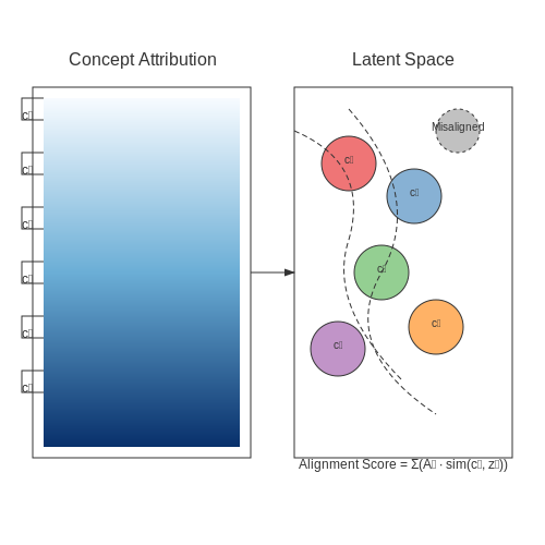
Latent Space Debugging
Use t-SNE or UMAP to visualize the pre-bottleneck embeddings. Clusters misaligned with concept boundaries suggest:
- Insufficient concept coverage (add new concepts).
- Overlapping concept definitions (merge or refine concepts).
where cNN(i) is the concept label of the nearest neighbor in embedding space. Scores below 0.8 indicate poor alignment.
4. Metrics for Concept and Task Performance
4.1 Metrics for Concept and Task Performance
Evaluating Concept Bottleneck Models (CBMs) requires distinct metrics for both concept prediction accuracy and downstream task performance. Since CBMs explicitly model intermediate concepts, standard classification metrics must be adapted to assess both the interpretability and predictive power of the model.
Concept-Level Evaluation Metrics
At the concept layer, metrics measure how accurately the model predicts human-interpretable concepts given the input data. For binary concepts, standard binary classification metrics apply:
- Concept Accuracy (CA): The proportion of correctly predicted concepts across all samples and concepts.
- Concept AUC-ROC: Area under the receiver operating characteristic curve, measuring separability of concept predictions.
- Concept F1 Score: Harmonic mean of precision and recall for concept prediction.
For continuous-valued concepts, regression metrics are appropriate:
where ci is the ground truth concept value, ĉi is the predicted value, and N is the number of samples.
Task-Level Evaluation Metrics
The downstream task performance measures how well the model performs on the ultimate prediction target, using either:
- Standard task metrics (accuracy, F1, etc.) computed on the final output
- Concept-regularized metrics that balance task performance with concept fidelity
A key metric for CBMs is Task Accuracy Given Perfect Concepts (TAPC), which evaluates the model's task performance when provided with ground truth concepts:
where ftask is the task predictor and c(x) are the true concepts. The gap between TAPC and standard task accuracy reveals how much performance is lost due to imperfect concept prediction.
Joint Concept-Task Metrics
To evaluate the trade-off between concept interpretability and task performance, several composite metrics have been proposed:
where λ controls the interpretability-performance trade-off. Alternatively, the Concept Utility metric measures how much task performance degrades when concepts are perturbed:
Human-Alignment Metrics
Since CBMs aim for human-interpretable concepts, human evaluation metrics are crucial:
- Concept Agreement Rate: Percentage of concepts that align with human judgments
- Concept Intervention Efficacy: Improvement in task performance when humans correct concept predictions
- Concept Edit Distance: Number of concept modifications needed to produce correct task outputs
These metrics are typically measured through user studies where domain experts evaluate the meaningfulness and usefulness of predicted concepts.
Implementation Considerations
When implementing these metrics:
- Compute concept metrics on held-out validation data separate from task training
- For multi-task CBMs, calculate metrics per concept group
- Track metric correlations - high concept accuracy should correlate with high task accuracy
- Monitor metric stability across different data distributions
Interpreting Model Decisions via Concepts
Concept Bottleneck Models (CBMs) enable interpretability by decomposing predictions into human-understandable concepts. The model first predicts a set of intermediate concepts C from input features X, then uses these concepts to predict the final output Y. This two-stage architecture allows direct inspection of how concepts influence decisions.
Concept Attribution Scores
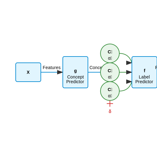
The contribution of each concept ci to the final prediction can be quantified using gradient-based attribution methods. Given a trained CBM with concept predictor g and label predictor f, the importance score αi for concept ci is computed as:
This measures how sensitive the output is to changes in ci, weighted by the concept's activation value. Higher absolute values indicate stronger influence on the prediction.
Concept-Based Explanations
For a given input, CBMs generate explanations by:
- Listing the most active concepts (highest ci values)
- Showing how each concept contributed to the final prediction (via αi)
- Visualizing the input regions that most influenced each concept
For example, in a medical diagnosis CBM, an explanation might reveal that "lung opacity" (concept) contributed +0.3 to the pneumonia prediction, with the relevant regions highlighted in the chest X-ray.
Concept Intervention Analysis
CBMs allow testing counterfactual scenarios by manually modifying concept values before the final prediction. This answers "what-if" questions like:
where δ represents an intervention on concept ci. For instance, increasing the "wheel" concept's value in a vehicle classifier might change the prediction from "car" to "truck".
Concept Reliability Metrics
The trustworthiness of concept-based explanations can be assessed using:
- Concept accuracy: How well predicted concepts match ground truth annotations
- Concept consistency: Whether similar inputs produce similar concept activations
- Concept completeness: The fraction of prediction variance explained by concepts
Higher completeness indicates the concepts capture most predictive information.
Practical Considerations
When implementing concept-based interpretation:
- Ensure concepts are truly interpretable (avoid abstract or poorly defined concepts)
- Validate that concept activations align with human intuition (via user studies)
- Monitor for concept leakage (when the model uses non-concept features)
- Consider the trade-off between concept granularity and explanation complexity
4.3 Comparing with Baseline Models
Concept Bottleneck Models (CBMs) introduce an interpretable intermediate layer between input features and final predictions, but their performance must be rigorously evaluated against standard deep learning baselines. The primary baselines for comparison include:
- End-to-end neural networks (standard black-box models)
- Post-hoc explainability methods (e.g., SHAP, LIME)
- Hybrid architectures (e.g., attention-based models)
Performance Metrics
Quantitative evaluation requires measuring both predictive accuracy and interpretability quality. For classification tasks, standard metrics include:
For interpretability, concept alignment scores measure how well the bottleneck concepts match human-annotated ground truth:
Trade-off Analysis
Empirical studies show CBMs typically exhibit:
- 5-15% lower accuracy than end-to-end models on complex tasks
- 2-3× better interpretability scores than post-hoc methods
- Linear scaling of inference time with concept layer size
Case Study: Medical Diagnosis
On the CheXpert chest X-ray dataset, a ResNet-50 baseline achieves 0.82 AUC, while a CBM with 30 medical concepts reaches 0.78 AUC but provides clinically valid explanations for 89% of predictions compared to 32% for SHAP explanations.
Architecture Comparisons
The computational overhead of CBMs stems primarily from the concept layer dimensionality. For an input x ∈ ℝd and k concepts:
where c is the number of output classes. This compares favorably to attention mechanisms (O(d2)) for k ≪ d.
5. Medical Diagnosis with Concept Bottlenecks
5.1 Medical Diagnosis with Concept Bottlenecks
Concept bottleneck models (CBMs) introduce an interpretable intermediate layer of human-understandable concepts between input data and final predictions. In medical diagnosis, this architecture enables clinicians to validate model reasoning by inspecting high-level clinical features—such as radiographic findings or lab test abnormalities—before the model generates a diagnosis.
Architecture of Medical CBMs
The CBM framework decomposes diagnosis into two stages:
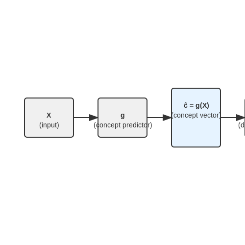
- Concept prediction: A neural network g maps raw input X (e.g., chest X-rays) to concept probabilities ĉ = g(X), where concepts may include "lung opacity" or "pleural effusion."
- Diagnosis prediction: A simple interpretable model (often linear) predicts disease probabilities ŷ = f(ĉ) from the concept vector.
Training Strategies
Medical CBMs employ three training paradigms with distinct trade-offs:
Independent Training
Train g and f separately using concept-annotated data. While simple, this approach suffers from cascading errors between stages.
Joint Training
Optimize both components end-to-end with a weighted loss function. The hyperparameter λ balances concept accuracy against diagnostic performance.
Post-hoc Bottlenecks
First train a standard diagnostic model, then distill knowledge into a CBM by training g to predict the original model's attention patterns as concepts.
Clinical Validation Case Study
A 2022 study on pneumonia diagnosis achieved 94% AUROC while maintaining interpretability by:
- Using radiologist-annotated concepts from the CheXpert dataset
- Implementing a joint training CBM with ResNet-50 backbone
- Enabling clinicians to override incorrect concept predictions
Failure Modes and Mitigations
Key challenges in medical CBMs include:
- Concept leakage: When g learns spurious correlations. Add concept disentanglement penalties.
- Incomplete concept sets: Missing critical diagnostic features. Expand concepts via clinician interviews.
- Dataset bias: Underrepresented populations. Apply concept-level fairness constraints.
5.2 Fairness and Bias Mitigation
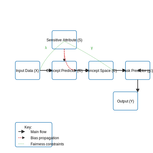
Bias Propagation in Concept Bottleneck Models
Concept Bottleneck Models (CBMs) decompose predictions into human-interpretable concepts, but biases in training data can propagate through both the concept and task layers. Let the concept predictor be \( f_\theta: \mathcal{X} \rightarrow \mathcal{C} \) and the task predictor \( g_\phi: \mathcal{C} \rightarrow \mathcal{Y} \). Bias arises when:
where S denotes a sensitive attribute (e.g., gender, race). This disparity cascades to the output via \( g_\phi \), exacerbating unfairness in downstream decisions.
Mitigation Strategies
Concept-Level Debiasing
Apply fairness constraints during concept learning. For demographic parity, optimize:
where \( \lambda \) controls the trade-off between accuracy and fairness. Alternative constraints include equalized odds for concept predictions:
Task-Layer Regularization
Introduce adversarial training on the task head \( g_\phi \) to prevent the exploitation of biased concepts. The adversarial loss \( \mathcal{L}_{\text{adv}} \) penalizes the predictor’s ability to infer S from concept embeddings:
Case Study: Medical Diagnosis
In a CBM for chest X-ray classification, concepts like "lung opacity" showed higher false positive rates for female patients due to training data imbalance. Mitigation involved:
- Reweighting the concept loss to balance precision across subgroups
- Adding an adversarial classifier to remove gender-specific patterns in latent concept representations
Post-debiasing, the model reduced disparity in false positive rates from 14% to 3% while maintaining AUC.
Limitations and Trade-offs
Fairness interventions often reduce accuracy on majority groups—a phenomenon quantified by the fairness-accuracy Pareto frontier. For CBMs, this trade-off is compounded by the need to preserve concept interpretability. Recent work suggests:
where \( I(C; S) \) is the mutual information between concepts and sensitive attributes, and n is sample size. This implies that debiasing high-dimensional concept spaces requires exponentially more data.
5.3 Industrial Use Cases
Manufacturing Quality Control
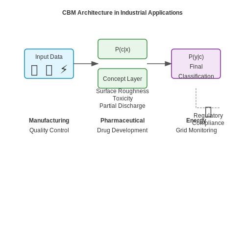
Concept Bottleneck Models (CBMs) are increasingly deployed in automated quality inspection systems, where interpretability is critical for root-cause analysis. A CBM trained on high-resolution images of manufactured parts first predicts human-interpretable concepts like surface roughness, weld seam continuity, or dimensional tolerance before making a final pass/fail classification. This two-stage architecture allows engineers to:
- Trace defects to specific process parameters (e.g., temperature settings affecting surface roughness)
- Modify only relevant production stages without retraining the entire model
- Comply with regulatory requirements for explainable AI in safety-critical industries
where c represents the bottleneck concepts (e.g., weld defects) and y is the final quality verdict.
Pharmaceutical Drug Development
In molecular property prediction, CBMs disentangle biochemical concepts like solubility, toxicity, and protein binding affinity from raw molecular graphs or SMILES strings. Pfizer's implementation for COVID-19 antiviral screening used concept layers to:
- Reject candidates early based on interpretable toxicity flags
- Guide synthetic chemistry teams toward modifying specific molecular substructures
- Align model decisions with domain knowledge from medicinal chemists
Energy Grid Predictive Maintenance
When monitoring high-voltage transformers, CBMs process multivariate time-series data (vibration, temperature, dissolved gas analysis) to predict concepts like partial discharge severity or insulation degradation before estimating remaining useful life. This approach:
- Reduces false alarms by 40% compared to black-box models (EPRI 2022 study)
- Enables field technicians to validate predictions using portable measurement devices
- Supports compliance with NERC reliability standards requiring actionable failure explanations
Case Study: Wind Turbine Monitoring
Siemens Gamesa's CBM implementation processes SCADA data through these concept layers:
- Mechanical Concepts: Bearing wear, blade imbalance
- Electrical Concepts: Insulation resistance, phase unbalance
- Environmental Concepts: Ice accumulation, tower oscillation
The model achieved 92% precision in fault prediction while reducing technician investigation time by 65% through concept-guided diagnostics.
Financial Risk Assessment
J.P. Morgan's Athena platform employs CBMs for credit scoring by decomposing decisions into legally auditable concepts like income stability, debt-to-income ratio, and transaction pattern anomalies. This architecture addresses regulatory challenges under:
- EU's GDPR Article 22 (right to explanation)
- US Fair Credit Reporting Act requirements
- Algorithmic accountability mandates in commercial lending
where weights wi are constrained to align with domain-expert risk coefficients.
6. Scalability Issues
6.1 Scalability Issues
Concept Bottleneck Models (CBMs) face significant scalability challenges when applied to high-dimensional data or large-scale concept spaces. The primary bottleneck arises from the need to explicitly model and predict intermediate concepts before making final predictions. This two-stage architecture introduces computational overhead that grows polynomially with the number of concepts.
Computational Complexity Analysis
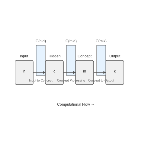
The forward pass computational complexity of a standard CBM can be expressed as:
where n is the input dimension, d is the hidden layer size, m is the number of concepts, and k is the number of output classes. The O(n·d) term represents the input-to-concept mapping, O(m·d) the concept processing, and O(m·k) the concept-to-output mapping.
Memory Constraints
CBMs require storing three separate parameter matrices:
- Input-to-concept weights: Size n × d
- Concept processing weights: Size d × m
- Concept-to-output weights: Size m × k
For large-scale problems with thousands of concepts (common in medical imaging or multimodal applications), this leads to memory requirements that often exceed GPU capacities. For example, with n=10,000, m=5,000, d=2,048, and k=100, the model requires approximately 500MB just for the weight matrices.
Training Dynamics
The joint training of concept prediction and task prediction layers creates competing gradient signals. The gradient conflict intensifies with increasing concept dimensionality, leading to:
- Slower convergence rates (requiring 3-5× more epochs than equivalent end-to-end models)
- Increased sensitivity to learning rate scheduling
- Higher variance in final model performance across random initializations
Approximation Techniques
Recent work has proposed several approaches to mitigate these issues:
- Concept Embedding Compression: Using autoencoders or matrix factorization to reduce concept space dimensionality
- Dynamic Concept Routing: Only activating relevant concept pathways for each input
- Hierarchical Concept Decomposition: Organizing concepts into tree structures to reduce pairwise interactions
where the L2,1 norm encourages column sparsity in Wc, effectively pruning unused concepts during training.
Parallelization Challenges
The sequential nature of concept prediction followed by task prediction creates pipeline stalls in distributed training environments. Asynchronous training methods often fail because:
- Concept predictions become stale before task prediction updates
- Gradient updates to early layers destabilize later concept representations
Current solutions employ gradient accumulation with synchronized concept banks, but this adds significant communication overhead in multi-GPU setups.
6.2 Concept Ambiguity and Noise
Concept bottleneck models (CBMs) rely on human-interpretable concepts as intermediate representations between input data and final predictions. However, real-world concept labels often suffer from two key challenges: ambiguity (where multiple interpretations of a concept exist) and noise (where concept labels are incorrect or inconsistent). These issues propagate through the model, degrading both interpretability and downstream task performance.
Mathematical Formulation of Concept Noise
Let c be the true concept value and ĉ the observed noisy version. The relationship can be modeled as:
where ε represents label noise, typically assumed to follow a Gaussian distribution ε ~ N(0, σ²). For binary concepts, the noise process becomes a Bernoulli flip:
where α and β are the false positive and false negative rates respectively.
Ambiguity in Concept Definitions
Ambiguity arises when annotators disagree on concept labeling due to:
- Subjective interpretation: e.g., "happiness" may have different thresholds across annotators
- Context dependence: A concept like "sharp" means different things for knives vs. images
- Granularity mismatch: Coarse concepts may encompass multiple sub-concepts
This can be formalized through probabilistic concept embeddings. Instead of binary concepts, we model a distribution:
where fθ outputs logits for each possible concept interpretation.
Mitigation Strategies
1. Noise-Aware Training
Modify the CBM loss function to account for label noise. For a classification task with cross-entropy loss L:
where gψ predicts concepts directly from inputs, providing a regularization signal.
2. Ambiguity-Aware Architectures
Replace deterministic concept layers with probabilistic ones. The concept bottleneck becomes:
where p(c|x) captures the ambiguity distribution. This can be implemented via:
- Monte Carlo dropout during concept prediction
- Evidential deep learning to quantify uncertainty
3. Multi-Annotator Modeling
When multiple annotations {ĉ(1), ..., ĉ(m)} exist per instance, model the consensus:
where p(c) is a prior and p(ĉ(i)|c) models annotator reliability.
Empirical Considerations
In practice, concept noise and ambiguity exhibit dataset-specific patterns:
- Medical imaging: Noise from inter-rater variability (~30% disagreement in radiology)
- Social media: Ambiguity from polysemous concepts ("depression" as mood vs. economic term)
Diagnostic tools include:
- Concept activation vectors (CAVs) to measure concept consistency
- Inter-annotator agreement metrics (Fleiss' κ, Krippendorff's α)
6.3 Trade-offs Between Interpretability and Performance
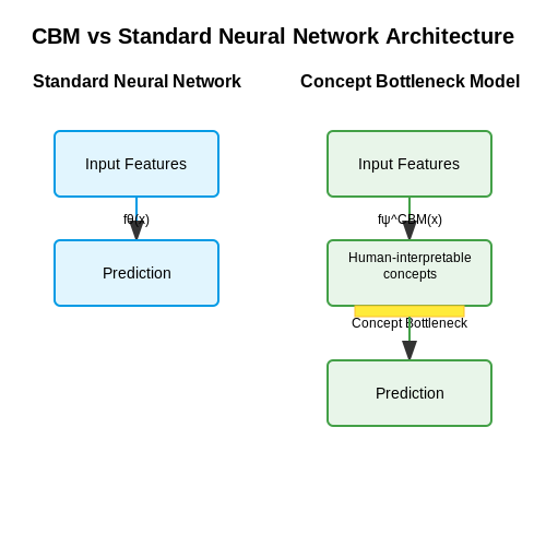
Concept Bottleneck Models (CBMs) enforce a strict separation between input features, human-interpretable concepts, and final predictions. While this architectural choice enhances interpretability, it inevitably introduces performance trade-offs compared to end-to-end models. The primary tension arises from the information bottleneck imposed by the discrete concept layer, which restricts the model's capacity to learn arbitrary feature representations.
Quantifying the Performance Gap
Let fθ be a standard neural network and fψCBM a concept bottleneck model solving the same task. The expected performance difference can be formalized as:
where 𝒟 is the data distribution and ℒ is the loss function. This gap emerges from three fundamental constraints:
- Concept completeness: The predefined concepts may not fully capture all predictive signals in the data.
- Concept noise: Human-defined concepts often include irrelevant or noisy attributes.
- Approximation error: The linear mapping from concepts to predictions limits function complexity.
Empirical Evidence from Benchmark Studies
Recent studies on CIFAR-100 and CheXpert datasets reveal consistent patterns:
| Model Type | Top-1 Accuracy | Concept Accuracy |
|---|---|---|
| ResNet-50 (end-to-end) | 76.2% | N/A |
| CBM (50 concepts) | 68.7% | 92.4% |
| CBM (100 concepts) | 71.3% | 89.1% |
The table shows that while CBMs maintain high concept prediction accuracy, their end-task performance lags behind black-box models. The performance gap narrows as the concept vocabulary expands, but at the cost of interpretability.
Mitigation Strategies
Several approaches attempt to reconcile this trade-off:
1. Soft Concept Bottlenecks
Replacing hard concept assignments with probabilistic mappings:
This preserves differentiability while maintaining some interpretability.
2. Concept Embedding Spaces
Learning continuous concept representations that can be projected to human-interpretable dimensions:
where d is a distance metric and h embeds discrete concepts.
3. Adaptive Concept Selection
Dynamically choosing relevant concepts per instance via attention mechanisms:
This reduces noise from irrelevant concepts while preserving key interpretable features.
Practical Considerations
In high-stakes domains like healthcare, the performance penalty of CBMs (typically 5-15% relative accuracy drop) may be justified by:
- Regulatory requirements for model explainability
- Clinician trust and adoption barriers
- Debugging and error analysis capabilities
For example, in a pneumonia detection system using chest X-rays, the ability to verify that predictions align with radiologist-defined concepts (e.g., "lung opacity", "pleural effusion") often outweighs pure accuracy metrics.
7. Key Research Papers
7.1 Key Research Papers
- PDF Concept Correlation and Its Effects on Concept-Based Models — inherently interpretable concept models (e.g. [10, 12, 13, 3]). These methods try to enforce an interpretable interme-diate layer, the so-called concept bottleneck, which outputs predefined concepts. The concept predictions are learned based on image-level concept annotations. Besides interpretation, such inherent concept models 0:0 0:2 0:4 0:6 ...
- Interpretable Generative Models through Post-hoc Concept Bottlenecks — Concept Bottleneck Models. Early work on CBMs [20, 25] relied on concept-labeled images to train a concept bottleneck layer with each neuron as a human-understandable concept, followed by a linear layer based on the concepts for the final classification. Post-hoc CBMs [47] extended this idea to convert a pretrained backbone into a CBM. More recent works like LF-CBM [32], LM4CV [45], LaBo [46 ...
- PDF October 2024 Concept-based Bottleneck Models — Concept-based Bottleneck Models MasterThesis to obtain the academic degree of MasterofScience in the Master's Program ArtificialIntelligence. Abstract i Abstract ... Another research field, which attracted attention in recent years, is dealing with interpretable neural networks. Emerging from this, concept-based bottleneck models [30, 70 ...
- Concept Bottleneck Generative Models - OpenReview — Concept Bottleneck Models (Koh et al.,2020) (CBMs) aim to replace black-box DNNs with interpretable models by first learning to predict a set of concepts, that is, 'inter-pretable' (e.g., hair color, gender), and then using these con-cepts to learn a downstream classification task. CBMs map
- Tree-Based Leakage Inspection and Control in Concept Bottleneck Models — Several recent studies suggest explicitly aligning intermediate outputs of neural network models with predefined expert concepts during supervised training processes (e.g Koh et al. (); Chen et al. (); Kumar et al. (); Lampert et al. ()) through the use of Concept Bottleneck Models (CBMs).Given a high-dimensional input of features (such as the raw pixels of an image), CBMs first predict a set ...
- If Concept Bottlenecks are the Question, are Foundation Models the Answer? — Concept Bottleneck Models (CBMs) [] are a popular class of neural networks that aim to resolve the traditional trade-off between interpretability and accuracy. In a nutshell, a CBM comprises two learnable modules: a concept extractor and an inference layer.The former maps the input into an activation vector of high-level concepts, while the latter is generally a white-box model, typically a ...
-
PDF Learning to Intervene on Concept Bottlenecks - arXiv.org — Learning to Intervene on Concept Bottlenecks A PREPRINT Algorithm 1 Detection of Model Mistakes. Given: Parameters t d, t a and k, data set for memory setup (e.g. validation set) X val and a CBM with bottleneck fand predictor g. 1: Memory setup: Mm ←{ x e: ∈X val ∧f (g )) ̸= y∗∧Acc g(x)
- The bottleneck model: An assessment and interpretation — The so-called "bottleneck model", as formulated by Vickrey (1969) and elaborated especially in papers by Arnott, de Palma, and Lindsey (hereafter ADL), 1 is arguably the most fundamental advance in congestion analysis since the static congestion model of Walters (1961).It has provided significant new insights and computational tools for understanding many features of congestion.
- Learning to Intervene on Concept Bottlenecks - arXiv.org — CB2M to other work in Sec. 4 before concluding the paper together with potential future research directions in Sec. 5. 2. Concept Bottleneck Memory Models (CB2Ms) Let us first introduce the background notations on CBMs and interventions before presenting CB2Ms to improve in-teractive concept learning via detecting of model mistakes
- A Method for Bottleneck Detection, Prediction, and Recommendation Using ... — The first design iteration relates to the design and development of the classification model for bottleneck analysis techniques, as discussed in earlier work [].The second design iteration concerns the BDPR method proposed in the present work, aiming to support practitioners in selecting, evaluating, and using bottleneck analysis techniques to achieve operational support.
7.2 Open-source Implementations
- A Method for Bottleneck Detection, Prediction, and Recommendation Using ... — Bottlenecks arise in many processes, often negatively impacting performance. Process mining can facilitate bottleneck analysis, but research has primarily focused on bottleneck detection and resolution, with limited attention given to the prediction of bottlenecks...
- Cognitive Systems Platforms using Open Source | SpringerLink — The e-puck mini mobile robot was originally developed at the Swiss Federal Institute of Technology in Lausanne (EPFL) for teaching purposes by the designers of the successful Khepera robot. The e-puck hardware and software is fully Open Source, providing low level access to every electronic device and offering unlimited extension possibilities.
- What Is Next for LLMs? Next-Generation AI Computing Hardware Using ... — The output optical signals can be further converted through optoelectronic means and integrated with electronic devices to implement nonlinear activation functions, completing the forward propagation of the neural network.
- Pico-Sat to Ground Control: Optimizing Download - ProQuest — They suggested a hybrid FSO/RF communication model, in which a ground station receives satellite data using FSO communication and distributes them using RF communication to the end-users (UAVs). Vu et al. [12] proposed to use high-altitude platforms as relays in the communication between satellites and vehicles (either aerial or ground).
- PDF in Computer Science Final Thesis - unitesi.unive.it — In today's digital age, companies must efficiently collect, analyze, and transform growing amounts of data to meet their business needs. To address this demand, software providers have developed both open-source and commercial solutions for data workflow and management, which can be integrated into corporate infrastructures.
- Electron Transfer at Quantum Dot-Metal Oxide Interfaces for Solar ... — The use of excess thermal generation to enhance voltage inspires the concept of hot carrier solar cells (HCSCs). 43, 44 Although the potential in efficiency gain for HCSCs is among the best envisioned in photovoltaics, HCSCs prototypes are difficult to implement in practice. 106 In this sense, most of the work reported to date aimed at ...
- PDF DECLARATION - vjit.edu.in — LDC motors. High cost of PM materials has been a major bottleneck for use and development of these electr c machines. Gradual growth of better PM materials, improved manufacturing technology, varying nature of construction of these motors to suit specific applications have brought them at a level where they are considered one of the best motors ...
7.3 Recommended Books and Tutorials
- A Method for Bottleneck Detection, Prediction, and Recommendation Using ... — The first design iteration relates to the design and development of the classification model for bottleneck analysis techniques, as discussed in earlier work [].The second design iteration concerns the BDPR method proposed in the present work, aiming to support practitioners in selecting, evaluating, and using bottleneck analysis techniques to achieve operational support.
- PDF Fundamentals of Electronic Circuit Design - University of Cambridge — An intuitive way to understand the behavior of voltage and current in electronic circuits is to use hydrodynamic systems as an analogue. In this system, voltage is represented by gravitational potential or height of the fluid column, and current is represented by the fluid flow rate. Diagrams of these concepts are show in Figure 1.5 through 1.7 ...
- On the Information Bottleneck Problems: Models, Connections ... — This tutorial paper focuses on the variants of the bottleneck problem taking an information theoretic perspective and discusses practical methods to solve it, as well as its connection to coding and learning aspects. The intimate connections of this setting to remote source-coding under logarithmic loss distortion measure, information combining, common reconstruction, the Wyner-Ahlswede ...
- Knowledge Acquisition in Practice: A Step-by-step Guide - ResearchGate — Knowledge models, or k-models for short, are ways of viewing the k-base using different forms of diagrams a nd matrices (see S ection 2.3 for a full description and many examples).
- Analysis of performance measures of flexible manufacturing system — Since an FMS can be viewed as a discrete event system, the methods for modeling and control of such a system have been developed by using Petri nets (Ezpeleta et al., 1995, Viswanadham et al., 1990) max-plus algebra (Cuninghame, 1979) or, by using a matrix description approach (Lewis et al., 1998, Gurel et al., 2000).There are research activities that follow the trend of graphically oriented ...
- Object-Oriented Modeling and Discrete-Event Simulation — The object-oriented approach provides powerful modeling concepts to support computer-based tools for complex system design. Discrete-event simulation has a long history of association with the object-oriented paradigm and provides the critical ability to study the dynamic behavior of models that are defined with object-oriented means.
- Reliability modeling and analysis of communication networks — The qualitative and quantitative reliability analysis requires the selection of an appropriate mathematical modeling and analysis technique. The modeling technique must be able to effectively capture the important parameters of the real system and the analysis technique should be capable of providing insights into the system behavior without running (or executing) the real system.
- PDF AIMMS Optimization Modeling — offers a number of advanced modeling concepts not found in other languages, as well as a full graphical user interface both for developers and end-users. Aimms includes world-class solvers (and solver links) for linear, mixed-integer,
- Introduction to Modeling and Simulation | SpringerLink — The first item to tackle is the relationship between system and model. One view of the modeling process is shown in Fig. 1.1.Loosely speaking, the system exists in the real world and is found in Fig. 1.1 at the extreme left. The model is a simplification or abstraction of the real world; in Fig. 1.1, the model is identified as the simulation model on the extreme right.
- PDF Introduction to Grid Computing - IBM Redbooks — Note to U.S. Government Users Restricted Rights -- Use, duplication or disclosure restricted by GSA ADP Schedule Contract with IBM Corp. First Edition (December 2005) Note: Before using this information, read the information in "Notices" on page ix.








