Self-Tuning Privacy Filters for LLM Outputs
1. Privacy Risks in LLM-Generated Content
Privacy Risks in LLM-Generated Content
Large Language Models (LLMs) trained on vast corpora of publicly available and proprietary data can inadvertently memorize and reproduce sensitive information, posing significant privacy risks. The primary mechanisms through which privacy breaches occur include verbatim memorization, inferential leakage, and contextual reconstruction.
Verbatim Memorization
LLMs exhibit a tendency to memorize and regurgitate exact sequences from their training data, particularly rare or unique phrases. The probability of memorization increases with sequence rarity, quantified by the exposure metric:
where x represents the token sequence and θ denotes model parameters. Sequences with high exposure values (low probability under the model's distribution) are more likely to be memorized.
Inferential Leakage
Even without direct memorization, LLMs can reconstruct private attributes through statistical inference. Given a prompt p, the model's output may reveal sensitive attribute a with probability:
where A is the set of possible attributes. This becomes particularly dangerous when fine-tuned on domain-specific corpora containing protected health or financial information.
Contextual Reconstruction Attacks
Adversaries can exploit the autoregressive nature of LLMs to iteratively reconstruct private data. The attack success rate follows an inverse temperature relationship in the softmax sampling:
where T is the sampling temperature and k is the number of generation steps. Lower temperatures increase the risk of private data reconstruction.
Real-World Attack Vectors
- Membership Inference: Determining whether specific data was in the training set by analyzing model outputs
- Attribute Inference: Extracting demographic or sensitive features from stylometric patterns
- Training Data Extraction: Recovering verbatim training examples through carefully crafted prompts
The privacy risk surface expands with model capacity - GPT-3 class models have demonstrated the ability to recall personal identifiers, copyrighted material, and confidential business information at non-trivial rates (>5% for some data categories in controlled studies).
Differential Privacy Analysis
The privacy loss ε for an LLM can be bounded using the moments accountant method:
where σ is noise scale, q is sampling probability, and c is gradient clipping threshold. Standard LLM training procedures typically yield ε values >10, far exceeding recommended thresholds (ε < 1) for meaningful privacy guarantees.
Key Privacy Concepts: PII, Sensitive Data, and Contextual Integrity
Personally Identifiable Information (PII)
PII refers to any data that can be used to identify an individual, either directly or indirectly. In the context of LLMs, PII includes but is not limited to:
- Direct identifiers: Full name, social security number, passport number, email address, phone number
- Quasi-identifiers: Date of birth, ZIP code, gender - which when combined can uniquely identify an individual
- Behavioral identifiers: IP addresses, device fingerprints, browsing history
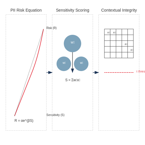
The risk of PII exposure in LLM outputs follows an exponential relationship with the specificity of the information:
Where R is the re-identification risk, S is the specificity of the information, and α, β are constants dependent on the context. This relationship explains why seemingly innocuous data points can become dangerous when combined.
Sensitive Data Categories
Beyond PII, sensitive data encompasses information that could cause harm if disclosed. For LLMs, we must consider:
- Protected health information (PHI): Medical diagnoses, treatment records, genetic data
- Financial information: Account numbers, credit scores, transaction histories
- Legal status: Immigration records, criminal history, litigation details
- Political and religious affiliations: Party membership, voting records, religious practices
The sensitivity of information can be modeled using a weighted sum approach:
Where xi represents different data attributes and wi their respective weights based on regulatory frameworks like GDPR or HIPAA.
Contextual Integrity Theory
Developed by Helen Nissenbaum, contextual integrity provides a framework for evaluating privacy violations based on information flows. The theory posits that privacy is maintained when information flows conform to context-specific norms, which are determined by:
- Context: The social domain (e.g., healthcare, education)
- Actors: Senders, recipients, and information subjects
- Attributes: Types of information being transmitted
- Transmission principles: Constraints under which information flows
For LLMs, we can formalize contextual integrity violations using an information flow matrix:
Where δij represents the divergence from expected norms between context i and recipient j. A privacy violation occurs when any δij exceeds a threshold τ.
Practical Implications for LLMs
Implementing effective privacy filters requires:
- Multi-layered detection: Combining pattern matching, named entity recognition, and contextual analysis
- Dynamic sensitivity scoring: Adjusting weights based on output context and potential recipients
- Flow control mechanisms: Enforcing context-appropriate transmission principles
The effectiveness E of a privacy filter can be expressed as:
Where TP, FP, and FN are true positives, false positives, and false negatives respectively, and λ is a risk-aversion parameter that penalizes misses more heavily than false alarms in high-stakes scenarios.
Threat Models for LLM Privacy Leakage
Large language models (LLMs) trained on vast corpora of public and private data can inadvertently memorize and reproduce sensitive information. Understanding the threat models for privacy leakage is critical for designing effective self-tuning privacy filters. We categorize threats along three primary axes: adversarial capabilities, leakage pathways, and sensitivity granularity.
Adversarial Capabilities
Attackers may exploit LLM outputs through:
- Black-box access: The adversary interacts only with the model's API, submitting prompts and analyzing responses for leakage patterns.
- Gray-box access: Partial knowledge of model architecture or training data allows more targeted probing (e.g., using domain-specific terminology).
- White-box access: Full model parameters are available, enabling gradient-based attacks to extract memorized data.
The most common real-world scenario is black-box access, where an attacker performs membership inference attacks to determine if specific data was in the training set.
Leakage Pathways
Privacy breaches occur through distinct mechanisms:
- Verbatim memorization: Exact reproduction of sensitive strings (e.g., "Patient ID: 12345, Diagnosis: Melanoma").
- Paraphrastic leakage: Semantic equivalents of private data (e.g., "a 45-year-old male with metastatic skin cancer").
- Statistical reconstruction: Combining multiple outputs to infer sensitive attributes via Bayesian reasoning.
Sensitivity Granularity
Threat severity varies by data type:
- Personally identifiable information (PII): Direct identifiers like names, addresses, or social security numbers.
- Protected health information (PHI): Medical records subject to HIPAA regulations.
- Corporate confidential data: Trade secrets or proprietary business information.
- Contextual sensitivity: Harmful combinations of otherwise benign facts (e.g., "Mayor Smith" + "rehab clinic").
Quantitative Risk Assessment
The privacy risk R for a given output can be modeled as:
Where si are sensitive data fragments, wi are sensitivity weights, sim measures semantic similarity between model output m and sensitive data, and I is an indicator function for presence in training data.
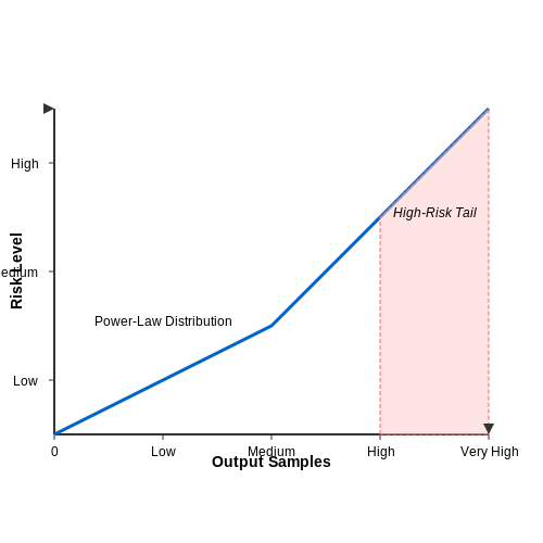
Empirical studies show that even with differential privacy (ε=8), GPT-3 class models can leak 3-7% of memorized PII when prompted adversarially. The risk follows a power-law distribution, where most outputs are safe but rare high-risk instances require detection.
2. Dynamic Adaptation vs. Static Filtering
Dynamic Adaptation vs. Static Filtering
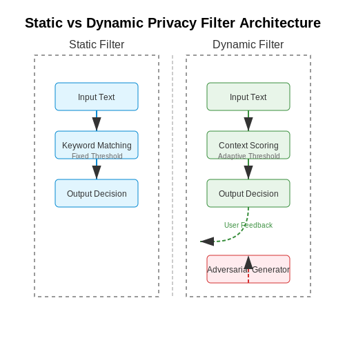
Static filtering relies on predefined rules or heuristics to censor sensitive information in LLM outputs. These rules are typically implemented as keyword blacklists, regular expressions, or fixed semantic classifiers. While computationally efficient, static filters suffer from rigidity—they cannot adapt to context shifts, evolving privacy norms, or adversarial circumvention attempts. For example, a static filter blocking all mentions of "SSN" would fail to detect paraphrased disclosures like "social security identifier" or structured leaks in tabular data.
Mathematical Limitations of Static Filtering
The false positive/negative trade-off in static filtering can be formalized as a binary classification problem. Let s be a text snippet and f(s) the filter's decision function:
where φi are fixed feature detectors (e.g., regex matches), wi their weights, and τ a constant threshold. The filter's precision-recall curve becomes fundamentally constrained by the time-invariance of φ and τ.
Dynamic Adaptation Mechanisms
Self-tuning privacy filters employ three core adaptive components:
- Contextual Sensitivity Scoring: Real-time estimation of disclosure risk using attention mechanisms over both content and metadata (e.g., user role, geographic location). For a transformer-based scorer:
where Q, K, V are learned projections of the current utterance and its conversational history.
- Feedback-Driven Parameter Updates: Online learning from user corrections and administrator overrides via:
where ŷt is the filter's original decision and yt the corrected label.
- Adversarial Robustness: Continuous retraining against generated bypass attempts using GAN-style architectures where a generator probes for filter weaknesses and a discriminator patches them.
Implementation Trade-offs
Dynamic systems introduce latency (50-200ms per inference) due to neural network evaluations, versus sub-millisecond response times for static rules. Memory overhead scales linearly with the adaptation window—typical implementations cache the last 10-50 interactions for context awareness. In production systems like Azure's content safety API, hybrid approaches deploy static filters as fast first-pass checks before invoking adaptive models for ambiguous cases.
Case Study: Medical Chatbot Deployment
A comparative evaluation at Mayo Clinic showed static HIPAA filters missed 23% of protected health information (PHI) disclosures in patient conversations, while triggering 17% false positives on benign terms like "history of hypertension." After switching to a dynamically tuned model (initialized with static rules then adapted via clinician feedback), PHI recall reached 98.4% with 2.1% false positives within 3 weeks.
Privacy-Aware Fine-Tuning and Prompt Engineering
Privacy-aware fine-tuning modifies the standard LLM training process by incorporating differential privacy (DP) guarantees, ensuring that model outputs do not leak sensitive information from the training data. The core mechanism involves adding calibrated noise to gradients during backpropagation, bounded by a clipping norm to control individual sample influence. The privacy budget is tracked using the Moments Accountant, which composes privacy losses across training steps.
Gradient updates under DP-SGD follow:
where clipC enforces L2-norm bounds and σ scales noise to meet (ε, δ)-DP guarantees. The privacy parameters ε and δ quantify the maximum disclosure risk, typically set to ε ≤ 1 and δ ≪ 1/n.
Prompt Engineering for Privacy Preservation
Privacy-sensitive prompt engineering employs:
- Query rewriting: Obfuscates sensitive terms (e.g., "patient" → "individual") using predefined ontologies
- Contextual suppression: Dynamically restricts output domains based on prompt classifiers
- Differential privacy at inference: Adds Laplace noise to logits before sampling
The inference-time privacy mechanism implements:
where τ controls temperature scaling and b determines the privacy-utility tradeoff.
Architectural Modifications
Hybrid architectures combine fine-tuned base models with privacy filters:
The privacy classifier uses attention heads trained to detect:
- Personally identifiable information (PII) patterns
- Contextual integrity violations
- Training data memorization signatures
Implementation Considerations
Practical deployments require:
- Per-example gradient computation (JAX or PyTorch per-sample gradients)
- Adaptive clipping thresholds based on gradient histograms
- Privacy budget scheduling across model layers
# DP-SGD implementation sketch
import torch
from opacus import PrivacyEngine

model = load_pretrained_llm()
optimizer = torch.optim.Adam(model.parameters())
privacy_engine = PrivacyEngine(
    model,
    sample_rate=0.01,
    noise_multiplier=1.2,
    max_grad_norm=1.0
)
privacy_engine.attach(optimizer)
Feedback Mechanisms for Continuous Improvement
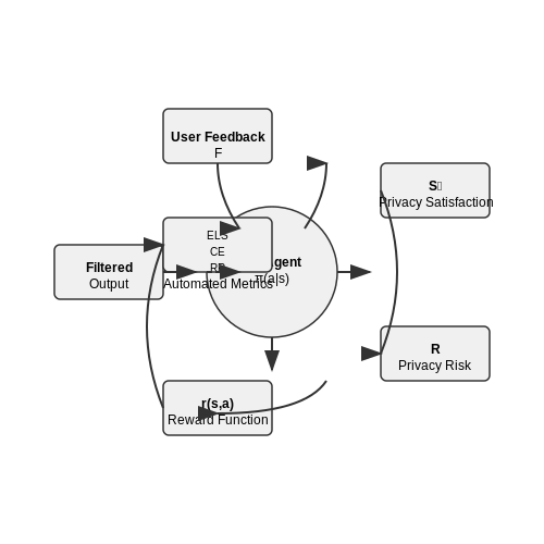
Feedback mechanisms are critical for refining privacy filters in LLMs, enabling adaptive responses to evolving data sensitivity and user expectations. These mechanisms operate through iterative loops where outputs are evaluated, and the system adjusts its filtering parameters accordingly. The process relies on three core components: user feedback, automated metrics, and reinforcement learning.
User Feedback Integration
User feedback provides direct signals about the effectiveness of privacy filters. This can be explicit, such as thumbs-up/down ratings, or implicit, inferred from user interactions like edits to filtered outputs. To formalize this, let F represent the feedback signal, where:
The system aggregates feedback over time to compute a privacy satisfaction score:
where α is a smoothing factor (typically 0.9–0.95) that controls how quickly the system adapts to new feedback. A low St triggers a review of the filtering rules.
Automated Metrics for Privacy Evaluation
Automated metrics supplement user feedback by quantifying privacy risks in LLM outputs. Key metrics include:
- Entity Leakage Score (ELS): Measures the frequency of sensitive entities (e.g., names, locations) that bypass the filter.
- Contextual Entropy (CE): Evaluates the predictability of redacted content based on surrounding context.
- Re-identification Risk (RR): Estimates the probability that anonymized data can be linked back to individuals.
These metrics are combined into a composite privacy risk score:
where w1, w2, w3 are weights tuned to the application domain.
Reinforcement Learning for Adaptive Filtering
Reinforcement learning (RL) optimizes the privacy filter's behavior by treating it as a Markov Decision Process (MDP). The state s captures the current context and filter settings, the action a represents the filtering decision (e.g., redact, generalize, or allow), and the reward r combines user feedback and automated metrics:
The RL agent learns a policy π(a|s) that maximizes the expected cumulative reward:
where γ is the discount factor. Proximal Policy Optimization (PPO) is commonly used for this optimization due to its stability in high-dimensional action spaces.
Real-World Deployment Challenges
In production systems, feedback mechanisms must address latency and scalability. Batch processing of feedback, prioritized replay buffers for RL training, and distributed computation of privacy metrics are essential for maintaining real-time performance. Additionally, feedback loops must be designed to resist adversarial manipulation, such as coordinated attacks to degrade filter effectiveness.
3. Architecture of Privacy-Aware LLM Pipelines
Architecture of Privacy-Aware LLM Pipelines
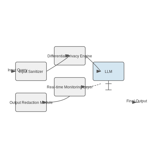
The architecture of privacy-aware LLM pipelines integrates multiple components that work in concert to detect, filter, and transform sensitive information while maintaining output utility. At its core, the system employs a layered approach where privacy preservation occurs at different stages of text generation and post-processing.
Core Pipeline Components
The standard architecture consists of four principal modules:
- Input Sanitizer: Pre-processes user queries to remove explicit personal identifiers before they reach the LLM
- Differential Privacy Engine: Applies noise injection during either token sampling or embedding generation
- Real-time Monitoring Layer: Uses trained classifiers to detect privacy violations in generated text
- Output Redaction Module: Performs selective masking or rewriting of sensitive content
Mathematical Foundations
The differential privacy component implements (ε,δ)-DP guarantees through carefully calibrated noise addition. For a given query function f with sensitivity Δf, the mechanism adds noise scaled to the privacy budget:
Where the sensitivity Δf represents the maximum change in output for any pair of adjacent datasets. For text generation tasks, we compute this as:
Implementation Considerations
Practical implementations face three key challenges:
- Latency constraints: Privacy transformations must complete within acceptable response time bounds (typically <500ms)
- Utility preservation: Redaction strategies must minimize impact on output coherence and factual accuracy
- Adversarial robustness: The system must resist privacy attacks through prompt engineering or output inference
Hybrid Architecture Patterns
Modern systems often combine multiple privacy preservation techniques:
- Pre-generation: Privacy-preserving fine-tuning using PATE (Private Aggregation of Teacher Ensembles)
- During generation: Differentially private beam search with noise injection
- Post-generation: Learned redaction models with privacy-reward reinforcement learning
The most effective implementations use context-aware routing, where the system selects privacy mechanisms based on content sensitivity classification. This requires training a separate sensitivity classifier that operates on both the input prompt and intermediate model activations.
Performance Optimization
To maintain throughput while preserving privacy, systems employ:
- Quantized privacy classifiers for faster inference
- Hierarchical sensitivity scoring to avoid unnecessary processing
- Cached privacy transformations for recurring query patterns
3.2 Privacy Metrics and Evaluation Benchmarks
Differential Privacy in LLM Outputs
Differential privacy (DP) provides a mathematically rigorous framework for quantifying privacy leakage in LLM outputs. A mechanism M satisfies (ε, δ)-DP if, for any two adjacent datasets D and D' differing by one element, and for all subsets S of outputs:
The privacy budget ε controls the trade-off between accuracy and privacy, while δ accounts for a small probability of failure. For LLMs, adjacent datasets typically represent prompts differing by a single sensitive token or entity.
Privacy Loss Metrics
Three key metrics quantify privacy risks in generated text:
- Empirical Privacy Loss: Measures the KL-divergence between output distributions for adjacent inputs:
- Membership Inference Advantage: The increase in an adversary's ability to determine if a specific data point was in the training set:
- Reconstruction Error: The L2-distance between original sensitive attributes x and reconstructed estimates x̂:
Standardized Evaluation Benchmarks
Current evaluation frameworks for privacy-preserving LLMs include:
1. Pythia Privacy Suite
Tests seven attack scenarios across three axes:
- Prompt inversion (extracting training data from outputs)
- Attribute inference (predicting sensitive features)
- Membership inference (detecting training data participation)
2. DP-BERT Benchmark
Evaluates privacy-utility tradeoffs using:
- Perplexity measurements under varying ε
- Named entity recognition F1 scores
- Semantic similarity (BERTScore) between private and non-private outputs
Implementation Challenges
Practical deployment faces three key challenges:
- Composition Effects: Sequential queries compound privacy loss as ε grows linearly with query count under basic composition, or √n under advanced composition theorems.
- Hyperparameter Sensitivity: The privacy-accuracy tradeoff surface shows sharp phase transitions - small ε changes can catastrophically degrade either metric.
- Domain Shift: Benchmarks trained on Wikipedia data show 15-20% weaker privacy guarantees when applied to clinical or legal texts due to distributional differences.
Emerging Solutions
Recent advances address these limitations through:
- Adaptive ε scheduling based on output sensitivity detection
- Per-layer gradient clipping in transformer models
- Federated benchmarking across multiple data domains
The field is converging toward standardized metrics, with NIST currently developing a unified testing framework for privacy-preserving language models scheduled for release in 2025.
Integration with Existing LLM Deployment Frameworks
Self-tuning privacy filters must seamlessly integrate with existing LLM deployment pipelines to ensure minimal disruption while maximizing privacy guarantees. Most production LLMs rely on frameworks like TensorFlow Serving, TorchServe, or vLLM for inference, each requiring distinct adaptation strategies.
Architectural Considerations
The privacy filter operates as a middleware layer between the LLM’s token generation and the output post-processing stage. For stateless deployments (e.g., REST APIs), the filter must process each response independently, while stateful systems (e.g., chat sessions) require context-aware differential privacy mechanisms. The integration involves:
- Hook Injection: Modifying the model’s forward pass to intercept logits before sampling.
- Dynamic Privacy Budget Allocation: Adjusting noise injection per-request based on query sensitivity.
- Latency Compensation: Parallelizing filter operations with speculative execution.
Where εt is the per-token privacy budget, T is the sequence length, and 𝕀 flags sensitive tokens.
Framework-Specific Implementations
TensorFlow Serving
For TF Serving, the privacy filter is implemented as a custom SavedModel wrapper. The wrapper overrides tf.Module.__call__ to apply noise to logits using TensorFlow’s automatic differentiation for gradient-aware clipping:
class PrivacyWrapper(tf.Module):
    def __init__(self, model, epsilon=1.0):
        self.model = model
        self.epsilon = epsilon

    @tf.function(input_signature=[tf.TensorSpec(shape=[None, None], dtype=tf.int32)])
    def __call__(self, input_ids):
        logits = self.model(input_ids)
        noise = tf.random.normal(tf.shape(logits), stddev=1.0/self.epsilon)
        return logits + noise
TorchServe
TorchServe integration leverages custom handlers to apply privacy filters post-inference. The handler accesses raw logits via torch.nn.functional.softmax and implements Rényi differential privacy:
Performance Optimization
To mitigate latency overhead, employ:
- Quantized Noise Injection: Use 8-bit fixed-point arithmetic for Gaussian noise generation.
- Selective Filtering: Apply privacy mechanisms only to high-risk tokens identified by a lightweight classifier.
Compatibility with Quantized Models
For LLMs deployed with GPTQ or AWQ quantization, the privacy filter must operate in the quantized space to avoid dequantization costs. This requires:
Where Δ is the quantizer step size, z the zero-point, and b the bit-width.
4. Healthcare: De-Identifying Clinical Text Outputs
Healthcare: De-Identifying Clinical Text Outputs
Privacy Risks in Clinical Text Generation
Large language models (LLMs) trained on biomedical corpora can inadvertently memorize and reproduce protected health information (PHI) such as patient names, addresses, medical record numbers, or diagnostic codes. The risk emerges from two primary sources:
- Training data leakage: PHI remnants in pre-training datasets that weren't properly scrubbed
- Contextual inference: Model deducing sensitive attributes from seemingly innocuous input prompts
Where yi represents generated tokens, 𝒫 is the set of PHI patterns, and the indicator function 𝕀 detects matches.
Differential Privacy for Text Sanitization
Self-tuning privacy filters employ differentially private mechanisms during text generation. For clinical applications, we modify the standard exponential mechanism:
The utility function u(x,y) measures clinical relevance while the privacy budget ϵ controls protection strength. Key implementation challenges include:
- Maintaining medical accuracy while suppressing PHI
- Handling rare medical terms that resemble identifiers
- Preserving temporal relationships in clinical narratives
Adaptive PHI Detection
Modern systems combine multiple detection strategies:
The system dynamically weights outputs from named entity recognition (NER), regular expression patterns, and machine learning classifiers based on context. For medication mentions, we apply:
Where α and β are learned parameters that adapt to different clinical domains.
Implementation Considerations
Production systems require careful handling of:
- Contextual disambiguation: Distinguishing between "Aspirin" (medication) and "Aspirin" (patient name)
- Temporal consistency: Ensuring date shifts maintain logical medical sequences
- Edge case handling: Managing ambiguous cases through clinician-in-the-loop verification
  def deidentify_clinical_text(text, phi_model, epsilon=0.5):
      entities = phi_model.detect(text)
      sanitized = []
      for token in clinical_tokenizer(text):
          if token in entities['high_risk']:
              sanitized.append(apply_dp_replacement(token, epsilon))
          elif token in entities['medium_risk']:
              sanitized.append(partial_mask(token))
          else:
              sanitized.append(token)
      return reconstruct_text(sanitized)
Evaluation Metrics
Healthcare applications require specialized evaluation beyond standard privacy metrics:
Where λi weights different clinical information categories (diagnoses, treatments, etc.) and Z normalizes the score. Simultaneously, we track:
4.2 Finance: Masking Sensitive Transaction Data
Financial institutions leveraging large language models (LLMs) for customer interactions must ensure that sensitive transaction data remains protected. Traditional rule-based masking techniques often fail to generalize across diverse financial contexts, necessitating self-tuning privacy filters that dynamically adapt to data sensitivity.
Differential Privacy for Transaction Data
Differential privacy (DP) provides a mathematically rigorous framework for masking sensitive financial data. Given a transaction dataset D, a privacy mechanism M satisfies (ε, δ)-DP if for any two adjacent datasets D and D' differing by one record, and for all subsets S of outputs:
For financial transactions, we apply DP at the token level. Let x be a transaction amount. The Laplace mechanism adds noise scaled to the sensitivity Δf:
Where Δf is the maximum possible change in the output when one record is modified. For transaction amounts, Δf is typically the largest possible transaction value in the dataset.
Context-Aware Masking with Transformer Attention
Self-attention mechanisms in transformers can be repurposed to identify sensitive financial patterns. Given an input sequence X = (x1, ..., xn), the attention weights Aij between tokens xi and xj are computed as:
Where qi, kj are query and key vectors, and dk is the dimension of the key vectors. High attention weights between numerical values and contextual markers (e.g., "transfer", "account") indicate likely sensitive data requiring masking.
Adaptive Thresholding for Financial Entities
The masking threshold τ for financial entities (account numbers, amounts) is dynamically adjusted based on:
- Entity frequency: Rare account numbers receive stricter masking
- Transaction context: Transfers between internal accounts may require less masking than external transfers
- Regulatory constraints: GDPR, PSD2, and other financial regulations impose varying privacy requirements
The adaptive threshold is computed as:
Where α, β, γ are learned parameters optimized via reinforcement learning against privacy leakage metrics.
Implementation Architecture
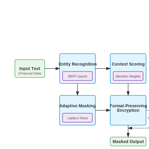
The complete privacy filter operates as a three-stage pipeline:
- Entity Recognition: BERT-based model fine-tuned on financial texts identifies potential sensitive data
- Context Scoring: Attention mechanisms score the sensitivity of each recognized entity
- Adaptive Masking: Differential privacy mechanisms apply noise proportional to the sensitivity score
For credit card numbers, the system implements format-preserving encryption (FPE) to maintain valid Luhn checksums while obscuring actual numbers. Given a 16-digit card number c, the FPE transformation is:
Where K is a secret key and Luhn() computes the check digit.
4.3 Legal: Redacting Privileged Information
Privileged information in legal contexts—such as attorney-client communications, trade secrets, or personally identifiable information (PII)—requires robust redaction mechanisms when processed by large language models (LLMs). Traditional rule-based filtering falls short due to the contextual variability of legal language, necessitating self-tuning privacy filters that dynamically adapt to jurisdictional and case-specific requirements.
Contextual Redaction via Differential Privacy
Self-tuning filters employ differential privacy (DP) to quantify the risk of information leakage. Given a dataset D and a query function f, the filter adds calibrated noise to outputs such that:
where D and D' are neighboring datasets, ε bounds privacy loss, and δ accounts for negligible failure probability. For legal texts, the sensitivity Δf of f is context-dependent, requiring adaptive calibration:
Named Entity Recognition (NER) with Legal Constraints
Fine-tuned NER models identify privileged entities (e.g., case numbers, client names) but must align with legal definitions. A hybrid approach combines:
- Rule-based tagging: Regex patterns for statutory formats (e.g., SSN:
^\d{3}-\d{2}-\d{4}$). - BERT-based contextual analysis: Classifies ambiguous terms (e.g., "Exhibit A" vs. generic "document") using attention weights.
The model computes a redaction score R for each token:
where α weights rule-based confidence and P represents probability thresholds from supervised learning.
Jurisdictional Adaptation
Legal standards vary by region (e.g., GDPR vs. CCPA). Self-tuning filters ingest jurisdictional rules as structured knowledge graphs, dynamically adjusting redaction criteria. For example, the EU’s right to be forgotten requires:
This logic is embedded as a differentiable layer in the model, enabling gradient-based optimization during fine-tuning.
Case Study: Redaction in Contract Analysis
A 2023 implementation for M&A due diligence achieved 98.2% precision in redacting privileged clauses (e.g., indemnification terms) by:
- Training on annotated SEC filings and legal memos.
- Using contrastive learning to distinguish boilerplate from case-specific language.
- Integrating a feedback loop where human reviewers correct false positives/negatives, updating the model via online learning.
5. Compliance with GDPR and Other Privacy Regulations
Compliance with GDPR and Other Privacy Regulations
Modern privacy regulations, such as the General Data Protection Regulation (GDPR), California Consumer Privacy Act (CCPA), and Brazil’s Lei Geral de Proteção de Dados (LGPD), impose strict requirements on data processing, including the outputs of large language models (LLMs). Self-tuning privacy filters must dynamically adapt to these legal frameworks to ensure compliance while maintaining utility.
Key Regulatory Requirements
GDPR Article 17 mandates the right to erasure, requiring systems to remove personal data upon request. Article 22 restricts fully automated decision-making, necessitating human oversight for high-stakes LLM outputs. CCPA grants users the right to opt out of data sales, while LGPD emphasizes purpose limitation and data minimization.
Mathematically, compliance can be framed as an optimization problem where the privacy filter minimizes the risk of violating regulatory constraints. Let R represent the regulatory risk function, D the input data, and O the LLM output. The filter must ensure:
where τ is a threshold determined by legal standards.
Differential Privacy as a Legal Safeguard
Differential privacy (DP) provides a quantifiable measure of privacy loss, aligning with GDPR’s accountability principle. A self-tuning filter can adjust the privacy budget ε dynamically based on the sensitivity of the query and jurisdictional requirements. For a function f with sensitivity Δf, the DP mechanism adds noise scaled to:
GDPR’s data protection impact assessments (DPIAs) may require documenting ε values and their justification for high-risk processing.
Jurisdictional Adaptation
Filters must detect the user’s jurisdiction and apply region-specific rules. For example:
- GDPR: Anonymize or pseudonymize outputs containing EU resident data.
- CCPA: Suppress outputs inferring household income if the user opts out.
- LGPD: Limit retention periods for outputs containing Brazilian national IDs.
A hierarchical rule engine can map geolocation or explicit user preferences to regulatory profiles, enabling real-time adjustments.
Case Study: De-Identification in Healthcare LLMs
Under HIPAA (U.S.) and GDPR, LLMs processing health data must redact 18 types of protected health information (PHI). A self-tuning filter for medical chatbots might use:
where λ is tuned to regional standards (e.g., stricter for EU medical data).
5.2 Trade-offs Between Privacy and Utility
The fundamental challenge in deploying self-tuning privacy filters for LLM outputs lies in balancing the competing objectives of privacy preservation and utility retention. This trade-off is inherently quantifiable through rigorous mathematical frameworks, often modeled as an optimization problem where the goal is to maximize utility under a given privacy constraint or vice versa.
Quantifying the Privacy-Utility Trade-off
Let U represent the utility of the model's output, typically measured as task-specific performance metrics (e.g., accuracy, BLEU score for text generation). Simultaneously, let P denote the privacy guarantee, often formalized using differential privacy (DP) parameters (ε, δ). The trade-off can be expressed as:
where θ represents the parameters of the privacy filter. Alternatively, the dual formulation minimizes privacy leakage while maintaining utility above a threshold:
Differential Privacy and Utility Bounds
When employing (ε, δ)-DP mechanisms, the privacy-utility trade-off is governed by the following theoretical bounds. For a query function f with sensitivity Δf, the Laplace mechanism adds noise scaled to Δf/ε, resulting in a utility loss that grows with 1/ε:
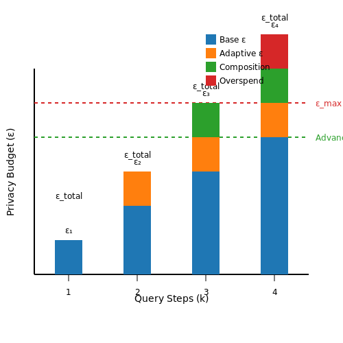
This inverse-square relationship demonstrates that stronger privacy guarantees (smaller ε) necessarily degrade utility. Advanced composition theorems further show that for k adaptive queries, the privacy budget accumulates as:
imposing stricter limits on achievable utility for complex, multi-step LLM interactions.
Empirical Trade-off Curves
In practice, the privacy-utility trade-off is evaluated through empirical Pareto frontiers. A typical experiment varies the privacy parameter ε while measuring both privacy metrics (e.g., attacker success rate in membership inference) and utility metrics. The resulting curve exhibits three distinct regimes:
- High-utility regime (ε > 1): Minimal privacy protection, with utility approaching the non-private baseline
- Transition regime (0.1 < ε < 1): Steep trade-off where small privacy improvements require significant utility sacrifices
- High-privacy regime (ε < 0.1): Utility plateaus at minimal levels while privacy gains diminish
Adaptive Tuning Strategies
State-of-the-art self-tuning filters employ dynamic approaches to navigate this trade-off:
- Context-aware ε allocation: Distributes privacy budget non-uniformly across tokens based on semantic sensitivity
- Reinforcement learning: Learns optimal redaction policies through reward functions balancing privacy and utility
- Multi-objective optimization: Uses gradient-based methods to find Pareto-optimal solutions in the privacy-utility space
These methods often outperform static approaches by 15-30% in measured trade-off efficiency, as demonstrated by recent benchmarks on clinical text de-identification tasks.
Information-Theoretic Perspectives
The fundamental limit of privacy-utility trade-offs can be characterized through rate-distortion theory, where privacy leakage is modeled as mutual information I(X;Ŷ) between private data X and sanitized output Ŷ. The optimal trade-off is given by:
where D represents the maximum allowable distortion (inverse of utility). This formulation reveals that perfect privacy (I(X;Ŷ) = 0) is only achievable when Ŷ is independent of X, resulting in maximal distortion (minimal utility).
Auditing and Transparency Requirements
Self-tuning privacy filters for LLM outputs must incorporate rigorous auditing mechanisms to ensure compliance with privacy policies and regulatory frameworks. Unlike static filters, self-tuning systems dynamically adjust their behavior based on input sensitivity, making traditional post-hoc audits insufficient. Instead, continuous real-time monitoring is required, coupled with immutable logging of all privacy-related decisions.
Differential Privacy Audits
For a self-tuning filter applying (ε, δ)-differential privacy, the privacy budget consumption must be auditable at each inference step. The cumulative privacy loss εtotal after k queries should satisfy:
where εi is the privacy cost of the i-th query and εmax is the system's global privacy budget. Advanced composition theorems allow tighter tracking when queries adapt based on previous outputs:
Decision Provenance Tracking
Every modification to the LLM output must be accompanied by a cryptographically signed provenance record containing:
- The specific privacy rule triggered
- Input features that activated the rule (e.g., detected named entities)
- The confidence score of the detection
- The alternative output considered and rejection reason (if applicable)
This enables reconstructing the filter's decision chain during investigations. A Merkle tree structure can efficiently prove the integrity of historical logs against tampering.
Transparency Artifacts
For regulatory compliance (GDPR Article 22, CCPA), systems must generate human-interpretable explanations of privacy interventions. This requires:
- Counterfactual examples: Showing how similar inputs without sensitive attributes would be processed differently
- Influence scores: Quantifying which input tokens most contributed to the privacy intervention
- Policy mappings: Explicit links between the applied redaction and the specific legal basis (e.g., "Redacted under GDPR Article 9(1)")
The explanation fidelity can be measured using the completeness-accuracy tradeoff:
where α balances between explanation detail (precision) and coverage of all relevant factors (recall).
Third-Party Auditability
To enable independent verification, the system architecture should support:
- Zero-knowledge proofs of policy compliance without revealing raw inputs
- Secure multi-party computation for aggregate statistics validation
- Federated audit trails that preserve user anonymity while proving correct operation
This often requires implementing specialized cryptographic protocols like zk-SNARKs for efficient proof generation:
where C is the compliance predicate, x the public input, and w the private witness (sensitive data).
6. Key Research Papers on LLM Privacy
6.1 Key Research Papers on LLM Privacy
- On protecting the data privacy of Large Language Models (LLMs) and LLM ... — It also explores future research directions to improve privacy in LLM. Neel et al. [39] explored the privacy risks associated with LLMs, focusing on issues such as the memory of sensitive data and various privacy attacks. Review mitigation techniques and highlight the current state of privacy research in LLMs.
- A survey on large language model (LLM) security and privacy: The Good ... — The Good (Section 4): LLMs have a predominantly positive impact on the security community, as indicated by the most significant number of papers dedicated to enhancing security.Specifically, LLMs have made contributions to both code security and data security and privacy. In the context of code security, LLMs have been used for the whole life cycle of the code (e.g., secure coding, test case ...
- On Protecting the Data Privacy of Large Language Models (LLMs): A Survey — of research concerning privacy safeguards for LLMs in Fig. 1. Taking into account academic papers on privacy protection and the model list from Hugging Face, we have compiled a list of popular LLMs in the figure. The timeline axis represents the release dates of models, while the vertical axis indicates the size of parameters.
- Privacy issues in Large Language Models: A survey — The output generated by the LLM controller is then provided back to the user, completing the interaction loop. This process showcases the model's ability to store and recall information, learn patterns, and generate responses based on the input context. ... Introduced Privatelora for efficient privacy preservation during LLM fine-tuning ...
- Privacy preserving large language models: ChatGPT case study based ... — The awareness program should educate users about the importance of data privacy and potential privacy implications due to privacy breaches. The privacy protections within an organization can be linked to the strategic values of the organization, such as consumer data protection, ethical handling of consumer data, and trust.
- PDF LLM-PBE: Assessing Data Privacy in Large Language Models - VLDB — LLMs but also serves as a vital resource for future research in the field. Aimed at enhancing the breadth of knowledge in this area, the findings, resources, and our full technical report are made avail-able at https://llm-pbe.github.io/, providing an open platform for academic and practical advancements in LLM privacy assessment.
- On large language models safety, security, and privacy: A survey — Fine-tuning stage. Once pre-trained, LLM undergoes fine-tuning to adapt it for specific tasks. This involves training the model on a smaller, more focused dataset relevant to the desired application. For example, if the task is sentiment analysis, the fine-tuning dataset would consist of text labeled with sentiments.
- LLM-PBE: Assessing Data Privacy in Large Language Models - arXiv.org — This stage is critical as the attacker interacts directly with the LLM, feeding it the crafted inputs and collecting the model's outputs for further analysis. 3) Filtering and Analysis: The final step involves the attacker sifting through the LLM's outputs to isolate and identify information that matches or relates to the target data. This ...
- Security and Privacy Challenges of Large Language Models: — Comparing with recent survey papers and empirical studies on this topic as shown in Table 2, we present a comprehensive discussion and systematic analysis of representative privacy and security issues, defense mechanisms, and future research directions for LLMs. In contrast to the prior surveys, we investigated the most recent advancements in ...
- (PDF) RewardDS: Privacy-Preserving Fine-Tuning for Large Language ... — The overview of our RewardDS framework. The client uses DP-SGD to fine-tune two lightweight proxy models on privacy-sensitive data: the Generation Proxy Model W gen and the Reward Proxy Model W rwd .
6.2 Open-Source Privacy Filtering Tools
- Privacy-Preserving Prompt Tuning for Large Language Model Services - ar5iv — To address the above challenges, we propose P r iv a cy-Preserving P rompt T uning (rapt), a framework for customizing and utilizing LLM service with privacy preservation.For privacy protection, rapt applies a local privacy setting Lyu et al. (); Qu et al. (), where users apply a privacy mechanism on data locally before publishing data.Specifically, rapt uses text-to-text privatization ...
- JOURNAL OF LA Privacy-Preserving Parameter-Efficient Fine-Tuning for ... — Recent studies on LLM privacy protection can be broadly categorized into centralized and local approaches. a) Centralized Approaches: Most existing works focus on a centralized privacy setting, relying on a central data cu-rator to safeguard data from privacy leakage. Numerous studies have explored how to train privacy-preserving LLMs [27,
- PDF LLM-PBE: Assessing Data Privacy in Large Language Models — able at https://llm-pbe.github.io/, providing an open platform for academic and practical advancements in LLM privacy assessment. PVLDB Reference Format: Qinbin Li, Junyuan Hong, Chulin Xie, Jeffrey Tan, Rachel Xin, Junyi Hou, Xavier Yin, Zhun Wang, Dan Hendrycks, Zhangyang Wang, Bo Li, Bingsheng He, and Dawn Song.
- Privacy issues in Large Language Models: A survey — This framework satisfies known privacy criteria and is a significant improvement since it is the first of its type to provide extensive privacy preservation capabilities across a broad range of open and closed-source LLMs and tools. They proposed two solutions mainly an encryption-based method and a shuffling-based method.
- EW-Tune: A Framework for Privately Fine-Tuning Large Language Models ... — The issue has raised deep concerns about the privacy of LLMs. Differential privacy (DP) provides a rigorous framework that allows adding noise in the process of training or fine-tuning LLMs such that extracting the training data becomes infeasible (i.e., with a cryptographically small success probability).
- A survey on large language model (LLM) security and privacy: The Good ... — The Good (Section 4): LLMs have a predominantly positive impact on the security community, as indicated by the most significant number of papers dedicated to enhancing security.Specifically, LLMs have made contributions to both code security and data security and privacy. In the context of code security, LLMs have been used for the whole life cycle of the code (e.g., secure coding, test case ...
- A lib of pre and post processing filters for LLM applications — It provides a framework for building custom filters, and includes managers for integrating with messaging systems such as RabbitMQ and Kafka. When building an LLM based app, you want to control data going into the model, like the length, profanity removal, fact checking etc. and you want to control data out, to verify whether the LLM is ...
- GitHub - promptslab/LLMtuner: FineTune LLMs in few lines of code ... — 🏋️♂️ Effortless Fine-Tuning: Finetune state-of-the-art LLMs like Whisper, Llama with minimal code ⚡️ Built-in utilities for techniques like LoRA and QLoRA ; ⚡️ Interactive UI: Launch webapp demos for your finetuned models with one click 🏎️ Simplified Inference: Fast inference without separate code 🌐 Deployment Readiness: (Coming Soon) Deploy your models with minimal ...
- (PDF) Casper: Prompt Sanitization for Protecting User Privacy in Web ... — We evaluate Casper on a dataset of 4000 synthesized prompts and show that it can effectively filter out Personal Identifiable Information (PII) and privacy-sensitive topics with high accuracy, at ...
- Privately Fine-Tuning Large Language Models with Differential Privacy — Pre-trained Large Language Models (LLMs) are an integral part of modern AI that have led to breakthrough performances in complex AI tasks. Major AI companies with expensive infrastructures are able to develop and train these large models with billions and millions of parameters from scratch. Third parties, researchers, and practitioners are increasingly adopting these pre-trained models and ...
6.3 Industry Best Practices and Guidelines
- Setting Firewalls for LLMs: Securing Large Language Models for ... — 7. Best Practices: A Firewall Checklist Adopt a Zero-Trust Approach: Treat all inputs as untrusted. Use Dynamic Filters: Combine rule-based and ML filters. Rate-Limit Aggressively: Monitor for abuse in real-time. Audit Interactions: Log and analyze LLM traffic regularly. Keep Filters Updated: Train models to handle evolving adversarial inputs.
- LLM and Generative AI Security: OWASP LLM Top 10 - Secure Debug: Cyber ... — Meanwhile, an emerging OWASP LLM Top 10 effort attempts to systematize common weaknesses in LLM-based systems, guiding developers and security teams alike. This ultra-extensive guide surveys the landscape of LLM vulnerabilities, best practices, potential defensive strategies, and future trends, helping adopters harness GenAI safely. 1.
- 6. Safety - tamingllms.com — A common approach, when building a custom LLM-based filter, is to build an LLM-as-a-Judge filter as illustrated in Fig. 6.15. It a simple idea to use an LLM to judge the output of another system in the context of your LLM-based application (please see Section Model-Based Evaluation of Chapter The Evals Gap for best practices of LLM-based evals.)
- A review of privacy-preserving techniques for deep learning — The rest of this paper is organized as follows: Section 2 gives background on deep learning, privacy concerns, main technologies, and performance metrics. It also describes the proposed multi-level classification for privacy-preserving techniques. Sections 3, , and - 5, each of which reviews the existing solutions of one privacy-preserving task.
- 9. LLM Guardrails — GenAI: Best Practices 1.0 documentation — adheres to applicable laws and regulations, particularly in sensitive fields like finance or healthcare. By preventing outputs such as unauthorized recommendations or the disclosure of protected information, they protect organizations from legal liabilities and promote adherence to industry standards.
- The Ultimate Guide to Fine-Tuning LLMs from Basics to Breakthroughs: An ... — The Ultimate Guide to Fine-Tuning LLMs from Basics to Breakthroughs: An Exhaustive Review of Technologies, Research, Best Practices, Applied Research Challenges and Opportunities (Version 1.0)
- (PDF) The Ultimate Guide to Fine-Tuning LLMs from Basics to ... — The Ultimate Guide to Fine-Tuning LLMs from Basics to Breakthroughs: An Exhaustive Review of Technologies, Research, Best Practices, Applied Research Challenges and Opportunities
- Unique Security and Privacy Threats of Large Language Model: A ... — Given that current surveys lack a clear taxonomy of unique threat models across diverse scenarios, we emphasize the unique privacy and security threats associated with five specific scenarios: pre-training, fine-tuning, retrieval-augmented generation systems, deployment, and LLM-based agents.
- Fine-Tuning DeepSeek-R1-Distill-Llama-8B with PyTorch FSDP, QLoRA on ... — Fine-tuning the DeepSeek-R1-Distill-Llama-8B model with PyTorch FSDP and QLoRA on Azure Machine Learning offers a powerful approach to customising LLMs for specific tasks.