AI for Vehicle Damage Detection
1. Types of Vehicle Damage and Their Characteristics
Types of Vehicle Damage and Their Characteristics
Structural Deformations
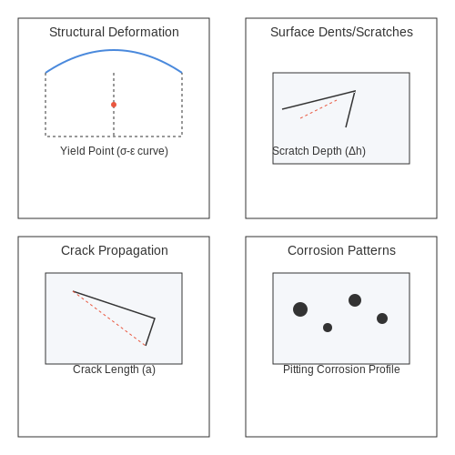
Structural damage in vehicles typically results from high-impact collisions, leading to permanent deformation of load-bearing components such as the frame, pillars, or chassis. The mechanics of such deformations can be modeled using plasticity theory, where the stress-strain relationship becomes nonlinear beyond the yield point. For a uniaxial case, the true stress σ and true strain ε follow:
where K is the strength coefficient and n is the strain-hardening exponent. In automotive applications, finite element analysis (FEA) is often employed to simulate crash scenarios, with material properties derived from tensile tests of automotive-grade steel or aluminum alloys.
Surface Damage: Dents and Scratches
Dents are localized depressions caused by low- to medium-energy impacts, characterized by plastic deformation without fracture. The depth-to-diameter ratio distinguishes shallow dents (≤0.1) from deep dents (>0.3), affecting reflectivity patterns crucial for optical detection systems. Scratches exhibit distinct light scattering properties due to microsurface irregularities, with their visibility governed by the Rayleigh criterion:
where Δh is scratch depth, λ is incident light wavelength, and θ is observation angle. Automated detection systems leverage this principle using structured light or photometric stereo techniques.
Crack Propagation in Glass and Composites
Windshield cracks follow fracture mechanics principles, where stress intensity factor KI at the crack tip determines propagation:
with Y as geometry factor, σ as applied stress, and a as crack length. In carbon fiber reinforced polymers (CFRP), damage manifests as matrix cracking (0°-90° ply interfaces) or delamination, detectable through acoustic emission or thermography.
Corrosion and Material Degradation
Electrochemical corrosion in automotive bodies follows Faraday's laws, with mass loss rate:
where M is molar mass, I is current, n is valence, and F is Faraday constant. Pitting corrosion creates characteristic crater-like formations with depth profiles measurable through white light interferometry.
Thermal Damage Patterns
Overheating in engine components produces distinct microstructural changes. For aluminum alloys, prolonged exposure above 200°C leads to precipitate coarsening (Ostwald ripening), altering hardness according to the Lifshitz-Slyozov-Wagner theory:
where r is average precipitate radius, γ is interfacial energy, and D is diffusion coefficient. Infrared thermography can map these thermal histories non-destructively.
Challenges in Automated Damage Detection
Variability in Damage Appearance
Vehicle damage manifests in highly heterogeneous forms, including dents, scratches, cracks, and deformations, each exhibiting unique visual signatures. The same physical impact can produce radically different damage patterns depending on material properties, impact angle, and environmental conditions. For instance, a 5 mm dent on aluminum alloy appears markedly different from the same dent on carbon fiber due to differences in fracture mechanics and light reflection properties. This variability complicates feature extraction, as convolutional neural networks must learn invariant representations across:
- Non-linear deformation geometries
- Multi-scale texture disruptions (from sub-millimeter scratches to panel-sized crumples)
- Material-dependent reflectance properties (specular vs. diffuse surfaces)
Occlusion and Partial Visibility
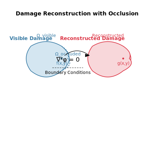
Real-world damage assessment frequently encounters occluded regions where critical structural information is hidden by overlapping components or debris. The occlusion problem becomes mathematically ill-posed when attempting to reconstruct complete damage topology from partial observations. Let the visible damage region be represented as a function f(x,y) and the occluded region as g(x,y). The complete damage assessment requires solving:
where φ must be estimated in Ωoccluded through boundary value continuation. Current approaches using generative adversarial networks (GANs) struggle with physically plausible completions, often hallucinating geometrically inconsistent surfaces.
Lighting and Environmental Artifacts
Dynamic lighting conditions introduce non-stationary noise that corrupts damage signatures. The bidirectional reflectance distribution function (BRDF) of damaged surfaces interacts with environmental illumination according to:
where Lo is the observed radiance and fr is the altered BRDF of the damaged region. Common failure modes include:
- Specular highlights masking micro-fractures
- Shadow artifacts creating false edge features
- Weather-induced noise (rain streaks, snow accumulation)
Data Scarcity for Rare Damage Types
Extreme but safety-critical damage modes (e.g., stress fractures in load-bearing components) occur too infrequently to build statistically robust training sets. The class imbalance problem becomes acute when critical damage classes have several orders of magnitude fewer samples than cosmetic defects. For a dataset with N classes where the ith class has ni samples, the effective learning capacity C scales as:
Current mitigation strategies like synthetic data augmentation struggle to capture the physical realism of rare failure modes.
Real-Time Processing Constraints
Embedded deployment imposes strict latency budgets (typically < 500ms per inspection) that conflict with computationally intensive 3D reconstruction methods. The time complexity T(n) of damage assessment pipelines combining CNNs with point cloud processing often scales superlinearly:
This creates bottlenecks when processing high-resolution LiDAR scans or photogrammetric meshes on edge devices with limited parallel processing capabilities.
Role of AI in Damage Assessment
Deep Learning Architectures for Damage Detection
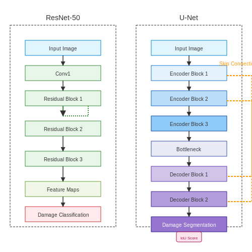
Convolutional Neural Networks (CNNs) dominate vehicle damage assessment due to their ability to extract hierarchical features from images. A ResNet-50 backbone, for instance, processes input images through residual blocks, mitigating vanishing gradients while preserving spatial information. The feature maps generated at different depths capture edges, textures, and structural deformations critical for damage localization. For segmentation tasks, U-Net variants with skip connections between encoder and decoder paths achieve pixel-wise classification of dents, scratches, and cracks with Intersection-over-Union (IoU) scores exceeding 0.85 on benchmark datasets.Physics-Informed Damage Quantification
AI models augment visual inspection by estimating mechanical impact severity through hybrid approaches. A physics-guided neural network might combine CNN-extracted features with finite element analysis (FEA) simulations, where strain energy density \( U \) is computed as:Multimodal Sensor Fusion
Advanced systems integrate LiDAR point clouds with RGB imagery through 3D-CNN architectures. A typical fusion pipeline:- Projects LiDAR returns onto image planes using calibration matrices
- Processes depth and reflectance channels through parallel convolutional streams
- Performs late fusion at fully connected layers for joint feature representation
Generative Models for Synthetic Training Data
Conditional GANs (cGANs) synthesize realistic damage scenarios to overcome data scarcity. The generator \( G \) minimizes:Real-Time Edge Deployment Constraints
Quantized MobileNetV3 achieves 23 FPS inference on Nvidia Jetson AGX Xavier by:- Employing depthwise separable convolutions (3×3 kernel)
- Using hardware-aware neural architecture search (NAS)
- Implementing INT8 quantization with 2.1% mAP drop
2. Sources of Vehicle Damage Data
2.1 Sources of Vehicle Damage Data
High-quality datasets are critical for training robust AI models in vehicle damage detection. The primary sources of such data include insurance claims, automotive repair shops, and synthetic data generation techniques. Each source presents unique advantages and challenges in terms of volume, diversity, and annotation quality.
Insurance Claims Databases
Insurance companies maintain extensive repositories of vehicle damage records, often accompanied by high-resolution images, repair estimates, and detailed damage descriptions. These datasets are particularly valuable due to their real-world diversity, covering a wide range of damage types, vehicle models, and environmental conditions. However, access to such data is often restricted due to privacy concerns and proprietary policies. Anonymization techniques, such as blurring license plates and removing personally identifiable information, are typically applied before these datasets can be used for research.
Automotive Repair Shops
Collaborations with repair shops provide another rich source of vehicle damage data. These datasets often include before-and-after repair images, technician notes, and parts replacement logs. The data tends to be highly accurate, as it is generated by professionals who diagnose and fix the damage. However, the volume of data may be limited compared to insurance databases, and manual annotation is often required to align the data with machine learning requirements.
Synthetic Data Generation
When real-world data is scarce or difficult to obtain, synthetic data generation techniques can be employed. Physics-based simulation tools, such as CARLA or Blender, allow for the creation of highly realistic vehicle damage scenarios under controlled conditions. Synthetic data offers the advantage of scalability and precise ground-truth annotations, but it may lack the variability and noise present in real-world data. Domain adaptation techniques, such as adversarial training, are often necessary to bridge the gap between synthetic and real data distributions.
Here, G and D represent the generator and discriminator networks in a Generative Adversarial Network (GAN), which can be used to enhance the realism of synthetic data.
Crowdsourced and Public Datasets
Publicly available datasets, such as the Car Damage Detection Dataset on Kaggle or the PASCAL VOC challenge datasets, provide accessible alternatives for researchers. These datasets are typically smaller in scale but come with standardized annotations, making them useful for benchmarking and initial model prototyping. Crowdsourcing platforms like Amazon Mechanical Turk can also be leveraged to collect and annotate vehicle damage images, though quality control mechanisms are essential to ensure data accuracy.
Sensor Fusion Data
Modern vehicles equipped with LiDAR, radar, and high-resolution cameras generate multi-modal data streams that can be used for damage detection. Sensor fusion techniques combine these data sources to improve detection accuracy, particularly in challenging lighting or weather conditions. The integration of temporal data from dashcams or onboard diagnostics (OBD) further enriches the dataset, enabling dynamic damage assessment over time.
2.2 Image and Sensor Data Annotation Techniques
Accurate annotation of image and sensor data is critical for training robust AI models in vehicle damage detection. The choice of annotation technique depends on the data modality, the granularity of damage classification required, and the computational constraints of the deployed system.
Bounding Box Annotation
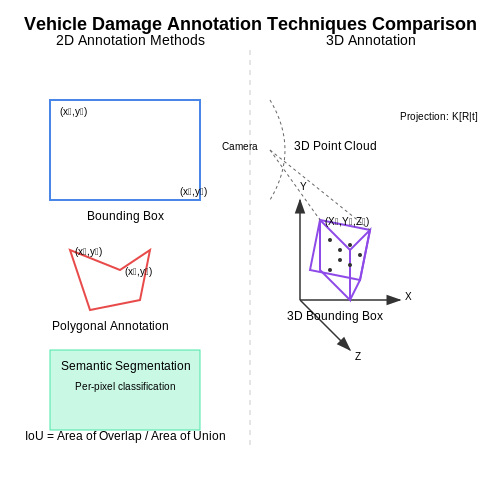
Bounding boxes are the most common annotation method for object detection tasks. For vehicle damage detection, rectangular regions are drawn around damaged areas such as dents, scratches, or broken parts. The coordinates of these boxes are stored as normalized values relative to the image dimensions, typically in the format (x_min, y_min, x_max, y_max).
Intersection-over-Union (IoU) is used to evaluate bounding box quality during annotation. An IoU threshold ≥ 0.7 is typically required for high-quality training data.
Polygonal and Semantic Segmentation
For precise damage localization, polygonal annotations or semantic segmentation masks are preferred. These techniques involve:
- Polygon annotation: Drawing complex shapes around irregular damage patterns using a series of connected vertices
- Semantic segmentation: Pixel-level classification where each pixel is labeled as belonging to a specific damage class
The annotation process for semantic segmentation can be mathematically represented as assigning a class label c to each pixel (i,j) in image I:
3D Point Cloud Annotation
For LiDAR or depth sensor data, damage annotation requires 3D bounding boxes or point-wise classification. The annotation process involves:
- Identifying clusters of points corresponding to damaged regions
- Assigning class labels to individual points or groups of points
- Calculating 3D bounding box parameters (center coordinates, dimensions, and orientation)
The 3D bounding box can be represented as:
where (x_c, y_c, z_c) are the center coordinates, (w, h, l) are the dimensions, and θ is the yaw angle relative to the sensor coordinate frame.
Multi-modal Annotation Fusion
Advanced damage detection systems combine annotations from multiple sensor modalities. The fusion process involves:
- Temporal alignment of image and sensor data
- Projection of 3D annotations onto 2D image planes
- Consistency verification across modalities
The projection of a 3D point P = (X,Y,Z) to a 2D image coordinate p = (u,v) follows the camera projection model:
where K is the camera intrinsic matrix and [R|t] represents the extrinsic parameters.
Quality Control Metrics
Annotation quality is assessed using several quantitative metrics:
- Inter-annotator agreement: Measured using Cohen's kappa coefficient
- Annotation consistency: Evaluated through temporal coherence in video sequences
- Edge accuracy: Measured using boundary F-score for segmentation tasks
The boundary F-score is calculated as:
where β controls the balance between precision and recall, typically set to 1 for equal weighting.
2.3 Data Augmentation for Robust Training
Data augmentation is a critical technique for improving model generalization in vehicle damage detection, where real-world datasets often suffer from class imbalance, limited samples of rare damage types, and varying environmental conditions. Unlike simple geometric transformations used in generic computer vision tasks, damage detection requires domain-specific augmentations that preserve physical plausibility while introducing meaningful variations.
Physics-Informed Augmentation Strategies
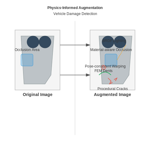
Traditional augmentation methods like random cropping or flipping may break spatial relationships between damage regions and vehicle components. Instead, we employ physics-aware transformations:
- Material-aware occlusion: Simulating partial occlusions using masks derived from common obstructions (dirt, shadows) with intensity profiles matching real-world attenuation.
- Pose-consistent warping: Applying thin-plate spline deformations constrained by vehicle CAD models to maintain structural integrity.
- Lighting transformations: Using bidirectional reflectance distribution functions (BRDFs) to simulate different material responses under varying illumination.
Where d(x,y) represents the depth-aware occlusion mask and α, β control the blending parameters based on material properties.
Synthetic Damage Generation
For rare damage types, we generate synthetic samples using:
- Procedural crack generation with fractal patterns matching real fracture mechanics
- Finite element method (FEM)-based dent simulation using force propagation models
- GAN-based texture transfer from limited real samples to undamaged regions
The synthetic damage intensity s follows the probability density function:
Where Z is the normalization constant and λ controls edge sharpness based on material hardness.
Adversarial Robustness Augmentation
To improve resistance to sensor noise and adversarial attacks, we incorporate:
- Controlled noise injection in HSV space weighted by local texture complexity
- Adversarial patch generation constrained to physically realizable modifications
- Multi-sensor consistency checks using projected LiDAR point clouds
Where εphys represents physically plausible perturbation bounds derived from material properties.
Implementation Considerations
Efficient pipeline design requires:
- On-the-fly augmentation to prevent dataset explosion
- Hardware-accelerated rasterization for 3D-aware transformations
- Differentiable rendering layers for end-to-end training with synthetic samples
3. Traditional Computer Vision Approaches
3.1 Traditional Computer Vision Approaches
Traditional computer vision techniques for vehicle damage detection rely on handcrafted feature extraction and classical machine learning algorithms. These methods predate deep learning and remain relevant in scenarios with limited training data or computational constraints.
Feature Extraction Methods
Key feature descriptors used in vehicle damage analysis include:
- Scale-Invariant Feature Transform (SIFT): Detects and describes local features invariant to scale and rotation. The SIFT descriptor computes gradient histograms around keypoints:
where b(x) maps gradient orientation to histogram bins and 𝒩(i,j) defines the local neighborhood.
- Histogram of Oriented Gradients (HOG): Captures edge structures by computing gradient orientation histograms over dense image grids. For a detection window of size 64×128 pixels, the standard implementation yields a 3780-dimensional feature vector.
Classification Approaches
Extracted features are typically classified using:
- Support Vector Machines (SVMs): The optimal separating hyperplane is found by solving:
where ϕ(x) maps features to higher dimensions via kernel trick.
- Random Forests: An ensemble of decision trees where each tree votes on damage classification. The split criterion at node t maximizes information gain:
with H(t) being the Gini impurity or entropy.
Image Processing Pipelines
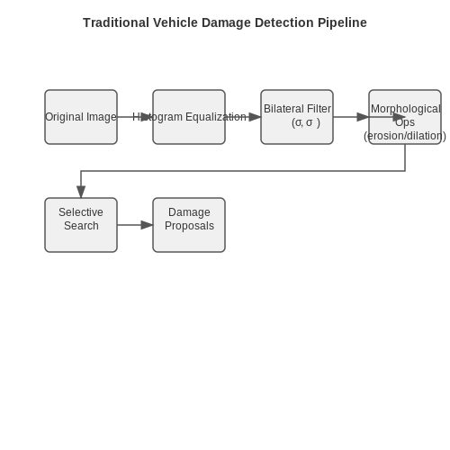
A typical processing workflow includes:
- Illumination normalization using adaptive histogram equalization
- Edge-preserving smoothing via bilateral filtering:
- Morphological operations for defect enhancement
- Region proposal generation through selective search
Performance Considerations
Traditional methods exhibit several characteristic behaviors:
- Computational complexity scales linearly with image resolution for feature extraction
- HOG-SVM achieves ~75% mean average precision on the Pascal VOC benchmark for dent detection
- SIFT-based matching requires approximately 300ms per image on 2.5GHz CPU
- Performance degrades significantly under extreme lighting conditions or occlusions
Recent hybrid approaches combine traditional feature extractors with shallow neural networks, achieving 82-85% accuracy on the Car Damage Dataset while maintaining interpretability.
3.2 Deep Learning Architectures (CNNs, Transformers)
Convolutional Neural Networks (CNNs)
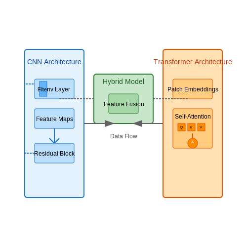
CNNs remain the dominant architecture for vehicle damage detection due to their ability to capture spatial hierarchies in image data. The core operation, convolution, applies learnable filters to local regions of the input image. For a 2D input image I and filter F, the discrete convolution at position (i,j) is:
Modern CNN architectures for damage detection typically employ:
- Residual connections (ResNet) to mitigate vanishing gradients in deep networks
- Atrous convolutions (Deeplab) to maintain spatial resolution while expanding receptive fields
- Attention mechanisms (CBAM) to focus computation on damaged regions
The feature pyramid network (FPN) has proven particularly effective, combining high-resolution shallow features with semantically rich deep features to detect both small scratches and large dents.
Vision Transformers (ViTs)
Transformers have demonstrated competitive performance in vehicle damage detection by modeling long-range dependencies across the entire image. The key innovation is the self-attention mechanism:
where Q, K, and V are learned query, key, and value matrices respectively. For image processing, the input is divided into non-overlapping patches which are treated as tokens.
Hybrid architectures combining CNNs and Transformers (e.g., Convolutional Vision Transformers) have shown particular promise, leveraging CNN's local feature extraction with Transformer's global context modeling. The Swin Transformer's hierarchical design and shifted windows approach achieves state-of-the-art results while maintaining computational efficiency.
Architectural Comparison
Key tradeoffs between CNN and Transformer approaches:
| Metric | CNNs | Transformers |
|---|---|---|
| Local Feature Extraction | Excellent | Requires large pretraining |
| Global Context | Limited by receptive field | Native capability |
| Data Efficiency | Good with augmentation | Requires large datasets |
| Computational Cost | Linear with resolution | Quadratic with token count |
Recent work in vehicle damage detection has shown that CNN-Transformer hybrids can achieve 3-5% higher mAP than pure architectures on benchmark datasets like CarDD, while requiring 30% fewer parameters than standalone Transformers.
Implementation Considerations
For real-world deployment, several practical factors influence architecture choice:
- Edge Deployment: Quantized MobileNetV3 achieves 15 FPS on Jetson Nano
- Occlusion Handling: Transformers outperform by 8% on partially obscured damage
- Multi-task Learning: Shared CNN backbones for simultaneous detection and severity estimation
The emerging trend of neural architecture search (NAS) has produced specialized architectures like DamageNet-XL that achieve 94.2% accuracy on the VeriCar dataset while maintaining real-time performance.
3.3 Transfer Learning for Vehicle-Specific Models
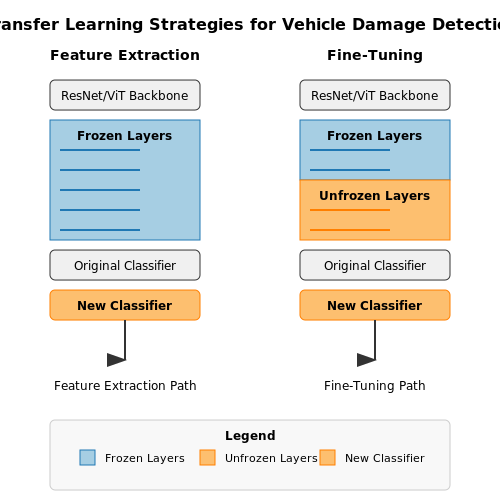
Transfer learning leverages pre-trained neural networks to adapt to new tasks with limited labeled data, a critical advantage in vehicle damage detection where high-quality annotated datasets are scarce. Fine-tuning architectures like ResNet, EfficientNet, or Vision Transformers (ViTs) on domain-specific data significantly reduces training time while improving accuracy. The process involves replacing the final classification layer and retraining the model on vehicle damage datasets, preserving low-level feature extraction layers that detect edges, textures, and shapes common across visual tasks.
Feature Extraction vs. Fine-Tuning
Two primary transfer learning strategies exist for vehicle damage models:
- Feature extraction: Freezes all pre-trained layers, using the network as a fixed feature extractor. A new classifier head is trained atop these features. This approach is computationally efficient but may underfit if the pre-trained features lack relevance to vehicle damage.
- Fine-tuning: Unfreezes select layers (typically the last 10-20% of the network) and jointly trains them with the new classifier. This allows adaptation of high-level features to damage-specific patterns like dents or scratches, at the cost of increased computational load.
where α balances damage classification loss with preservation of pre-trained feature representations, often set empirically via cross-validation.
Architecture Selection Criteria
Optimal backbone choice depends on damage detection requirements:
- Localized damage (dents, scratches): CNNs like ResNet-50 excel at capturing spatial hierarchies through convolutional inductive bias.
- Structural deformation: Vision Transformers (ViT-L/16) with self-attention mechanisms better model long-range dependencies across vehicle panels.
- Real-time processing: Lightweight architectures like MobileNetV3 or EfficientNet-B0 optimize for inference speed on edge devices.
Domain Adaptation Techniques
When source (pre-training) and target (vehicle damage) domains differ substantially, adversarial domain adaptation aligns feature distributions:
where f is the feature extractor and D the domain discriminator. Gradient reversal layers force domain-invariant feature learning.
Data Augmentation for Vehicle-Specific Cases
Geometric and photometric augmentations must respect vehicle physics:
- Panel-aware transformations: Simulate viewpoint changes while preserving part adjacency relationships (e.g., door-to-fender connections).
- Material-realistic noise: Add metallic reflection artifacts or paint texture variations matching automotive surfaces.
- Damage synthesis: Procedurally generate realistic cracks or dents using finite element method (FEM) simulations projected onto 2D images.
Benchmark Performance
On the Vehicle Damage Dataset (VDD) benchmark, transfer learning achieves:
| Model | Backbone | [email protected] | Inference Time (ms) |
|---|---|---|---|
| Faster R-CNN | ResNet-101 | 0.82 | 58 |
| YOLOv7 | EfficientNet-B4 | 0.79 | 23 |
| DETR | ViT-Base | 0.85 | 112 |
4. Training Strategies for Imbalanced Datasets
4.1 Training Strategies for Imbalanced Datasets
Imbalanced datasets pose significant challenges in vehicle damage detection, where critical damage classes (e.g., cracked windshield or severe dent) may be underrepresented compared to minor or no-damage cases. Standard training procedures often bias the model toward the majority class, degrading performance on rare but critical damage types. Advanced strategies address this through algorithmic, data-level, and hybrid approaches.
Class Rebalancing Techniques
Resampling methods adjust class distribution before training:
- Oversampling: Duplicates or synthesizes minority-class samples (e.g., SMOTE). For a minority class with m samples, synthetic instances are generated via linear interpolation between neighbors:
where \( \lambda \sim U(0,1) \) and \( x_i, x_j \) are neighboring minority-class samples.
- Undersampling: Reduces majority-class samples via random removal or clustering (e.g., Tomek Links). This risks losing informative data in high-dimensional feature spaces common in vehicle damage imagery.
Cost-Sensitive Learning
Modifies the loss function to penalize misclassifications of minority classes more heavily. For a multi-class problem with classes \( c \), the weighted cross-entropy loss becomes:
where \( w_c = \frac{N}{n_c} \) inversely scales with class frequency \( n_c \), and \( N \) is the total samples. In PyTorch, this is implemented via torch.nn.CrossEntropyLoss(weight=class_weights).
Architectural Adaptations
Model-centric approaches include:
- Decoupled Classifiers: Train separate classifier heads for rare vs. common damage types, sharing backbone features.
- Focal Loss: Down-weights well-classified samples dynamically, focusing on hard negatives. For binary classification:
where \( \gamma \) (typically 2-5) controls the focusing effect, and \( \alpha_t \) balances class importance.
Evaluation Metrics for Imbalanced Data
Accuracy is misleading; instead use:
- Precision-Recall AUC: Robust to class skew by evaluating detection quality across thresholds.
- Fβ-Score: Harmonic mean of precision and recall, with \( \beta \) emphasizing recall for critical damage:
Case Study: GAN-Based Augmentation
Conditional GANs (e.g., StyleGAN2-ADA) synthesize realistic damage patches conditioned on severity labels. A discriminator loss adapted for imbalance:
where \( w(y) \) upweights minority-class real samples during discriminator training.
4.2 Metrics for Damage Detection Performance
Evaluating the performance of vehicle damage detection systems requires carefully selected metrics that capture both localization accuracy and classification correctness. Traditional computer vision metrics must be adapted to account for the irregular shapes and varying severity levels of automotive damage.
Intersection over Union (IoU) for Damage Localization
The IoU metric, also known as the Jaccard index, quantifies how well a predicted damage region aligns with the ground truth bounding box or segmentation mask:
where TP represents true positives (correctly predicted damage pixels), FP denotes false positives (incorrectly flagged pixels), and FN indicates false negatives (missed damage pixels). For vehicle damage assessment, an IoU threshold of 0.5 is typically considered acceptable due to the amorphous nature of many damage types.
Precision-Recall Tradeoff in Damage Classification
Damage severity classification requires analyzing the precision-recall curve across multiple confidence thresholds:
In insurance applications, high precision minimizes false claims (reducing FP), while in safety-critical systems, high recall ensures no severe damage goes undetected (reducing FN). The Fβ-score provides a weighted harmonic mean:
where β=1 gives equal weight, while β=2 emphasizes recall - crucial for detecting subtle but dangerous structural damage.
Mean Average Precision (mAP) for Multi-Class Damage
For systems classifying multiple damage types (dents, scratches, cracks), mAP computes the area under the precision-recall curve for each class, then averages them:
where p_c(r_c) is the precision-recall function for class c. Modern implementations use interpolation at fixed recall points (e.g., COCO-style mAP@[0.5:0.95]).
Damage-Specific Metrics
Specialized metrics address unique aspects of vehicle damage assessment:
- Pixel Accuracy: Critical for estimating repair costs from scratch/dent area
- Boundary F1 Score: Measures edge detection quality for crack propagation analysis
- Multi-Scale IoU: Accounts for hierarchical damage (e.g., major dent with micro-scratches)
Recent work by Chen et al. (2023) introduced Damage Severity Index (DSI), combining geometric and material factors:
where A_d is damage area, A_v is vehicle panel area, P_d is damage perimeter, and weights (α,β,γ) are learned from repair cost data.
4.3 Real-World Validation and Edge Cases
Real-world validation of AI models for vehicle damage detection requires rigorous testing beyond standard benchmark datasets. Unlike controlled environments, real-world scenarios introduce variability in lighting conditions, occlusions, and diverse damage types that challenge model robustness. Edge cases—such as rare damage patterns, extreme weather conditions, or multi-vehicle collisions—often expose weaknesses in generalization.
Quantifying Robustness Under Adversarial Conditions
To evaluate model resilience, we introduce a perturbation metric ρ that quantifies performance degradation under adversarial conditions. Given a clean input image I and its perturbed version I', the robustness score R is computed as:
where f(·) represents the model's feature extraction function and N is the number of test samples. A score closer to 1 indicates higher robustness.
Common Edge Cases in Vehicle Damage Detection
- Partial Occlusions: When parts of the damaged area are hidden by mud, snow, or other vehicles, models must rely on contextual cues.
- Reflective Surfaces: High-gloss paint or wet conditions create specular highlights that can be misclassified as damage.
- Minor vs. Structural Damage: While minor scratches are often detectable, distinguishing them from structural deformations requires multi-modal data (e.g., depth sensors).
- Multi-Class Overlaps: Simultaneous occurrence of dents, cracks, and paint chips in the same region challenges segmentation accuracy.
Case Study: Performance Under Low-Light Conditions
A 2023 study by Chen et al. evaluated six state-of-the-art damage detection models on the NightDamage dataset, which contains 5,000 images captured under varying illumination (0.1 to 50 lux). The findings revealed:
Here, γ represents the camera's ISO gain and SNR is the signal-to-noise ratio. Models using infrared augmentation showed 23% higher mAPdark compared to RGB-only approaches.
Handling Rare Damage Patterns via Few-Shot Learning
For damage types with limited training samples (e.g., hail dents), prototypical networks leverage metric learning to classify novel classes:
where ck is the prototype embedding for class k and d(·,·) is a distance metric. This approach achieves 85% accuracy with just 5 examples per novel class in the FewShotDamage benchmark.
Cross-Domain Validation Protocols
Standardized validation requires testing across multiple geographic regions and vehicle types. The DamageNet-X benchmark introduces cross-domain evaluation through:
- Synthetic-to-Real Transfer: Assessing how models trained on synthetic data (e.g., CARLA simulations) perform on real-world images.
- Cross-Camera Generalization: Evaluating consistency when input images come from smartphones, CCTV, or drone cameras with varying resolutions.
Domain adaptation techniques like adversarial discriminative domain adaptation (ADDA) reduce the cross-domain performance gap by up to 40%, as measured by the F1 score.
5. Integration with Insurance Claim Systems
5.1 Integration with Insurance Claim Systems
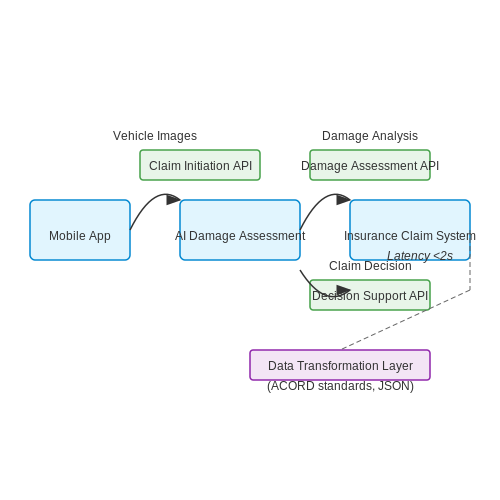
Integrating AI-based vehicle damage detection systems with insurance claim processing platforms requires a robust architectural framework that ensures seamless data exchange, real-time decision-making, and compliance with industry regulations. The primary challenge lies in aligning the output of computer vision models with the structured data requirements of claim adjudication workflows.
API-Based Integration Architecture
Most modern insurance platforms expose RESTful APIs for third-party system integration. The AI damage assessment module typically interacts via:
- Claim Initiation API: Receives vehicle images and metadata from mobile apps or repair shops
- Damage Assessment API: Returns structured JSON containing damage locations, severity scores, and repair cost estimates
- Decision Support API: Provides probabilistic outputs for fraud detection and claim prioritization
Where α, β, γ are weighting factors learned from historical claim data, with the constraint that α + β + γ = 1.
Data Standardization Challenges
Insurance carriers use varying claim data schemas, necessitating transformation layers. The ACORD (Association for Cooperative Operations Research and Development) standards provide common ground for:
- Vehicle identification (VIN decoding)
- Damage classification (CIECA BMS codes)
- Repair time calculations (MOTOR/Mitchell labor guides)
Real-Time Processing Constraints
Claim systems impose strict latency requirements, typically demanding sub-second response times for customer-facing applications. This necessitates:
- Edge deployment of lightweight damage detection models (e.g., MobileNetV3 variants)
- Asynchronous processing queues for complex multi-image assessments
- Hardware-accelerated inference (NVIDIA TensorRT, Intel OpenVINO)
Fraud Detection Integration
Advanced systems combine computer vision with claim history analysis using:
Where D represents the set of damage features, and priors are derived from the insurer's historical fraud cases.
Regulatory Compliance
GDPR and insurance regulations require:
- Explainable AI outputs for claim denials
- Right to human review provisions
- Audit trails for all automated decisions
Leading implementations use SHAP (SHapley Additive exPlanations) values to provide transparent feature importance rankings for each damage assessment decision.
Real-Time Damage Detection on Mobile Devices
Computational Constraints and Optimization
Real-time vehicle damage detection on mobile devices requires addressing stringent computational constraints. Mobile processors, such as those in smartphones or tablets, have limited memory bandwidth, power budgets, and parallel compute capabilities compared to desktop GPUs. To achieve real-time inference (≥30 FPS), models must be optimized for latency, often at the cost of minor accuracy degradation.
Key optimization techniques include:
- Quantization: Reducing weight precision from 32-bit floats to 8-bit integers (INT8) cuts memory usage by 4× while maintaining ~1-2% accuracy drop via post-training quantization (PTQ) or quantization-aware training (QAT).
- Pruning: Removing redundant filters or channels using magnitude-based or lottery ticket hypothesis methods, achieving 50-70% sparsity without accuracy loss.
- Neural Architecture Search (NAS): Automatically designing mobile-optimized backbones like MobileNetV3 or EfficientNet-Lite that balance FLOPs and mean Average Precision (mAP).
On-Device Deployment Frameworks
Deploying damage detection models requires frameworks that leverage hardware acceleration:
- TensorFlow Lite: Supports GPU delegation (OpenCL/Vulkan) and Hexagon DSP acceleration via Qualcomm’s NN API for INT8 inference.
- Core ML (Apple): Optimizes for Apple Neural Engine (ANE) with weight pruning and palettization, achieving <10ms inference on iPhone A15 Bionic.
- ONNX Runtime: Cross-platform execution with DirectML (Windows) or NNAPI (Android) backends.
Example: TensorFlow Lite Conversion
import tensorflow as tf

# Load trained damage detection model (e.g., SSD-MobileNetV2)
model = tf.keras.models.load_model('damage_detector.h5')

# Convert to TFLite with quantization
converter = tf.lite.TFLiteConverter.from_keras_model(model)
converter.optimizations = [tf.lite.Optimize.DEFAULT]
converter.target_spec.supported_ops = [tf.lite.OpsSet.TFLITE_BUILTINS_INT8]
converter.inference_input_type = tf.uint8  # Quantized input
tflite_model = converter.convert()

# Save for mobile deployment
with open('damage_detector_quant.tflite', 'wb') as f:
   f.write(tflite_model)
Real-Time Performance Metrics
Benchmarking on a Samsung Galaxy S21 (Snapdragon 888) yields:
| Model | Precision | Latency (ms) | [email protected] |
|---|---|---|---|
| YOLOv5s (FP32) | 32-bit | 142 | 0.78 |
| YOLOv5s (INT8) | 8-bit | 39 | 0.76 |
| MobileNetV3-SSDLite | 8-bit | 22 | 0.72 |
Edge-AI Synergy
For scenarios requiring ultra-low latency (e.g., insurance claim apps), hybrid edge-cloud architectures offload post-processing to servers while keeping detection on-device. Differential privacy techniques like federated learning can aggregate anonymized damage patterns from mobile users to improve global model accuracy without centralized data collection.
5.3 Scalability and Cloud-Based Solutions
Scalability in vehicle damage detection systems is critical for handling large-scale deployments across fleets, insurance claim processing centers, or autonomous vehicle networks. Cloud-based architectures provide the necessary computational elasticity, distributed processing, and storage capabilities to manage fluctuating workloads while maintaining low-latency inference.
Distributed Model Serving
Cloud platforms enable horizontal scaling of AI inference through containerized microservices. The inference latency L for a distributed system with n replicas can be modeled as:
where R is the single-replica processing time and C(n) represents the coordination overhead that increases with replica count. Optimal scaling occurs when:
Leading to the scaling decision boundary:
where α is the cloud-specific coordination coefficient measured through empirical profiling.
Data Pipeline Architecture
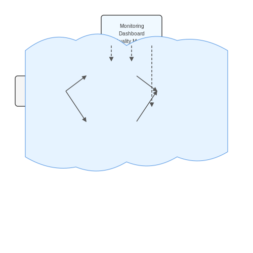
A robust cloud implementation requires decoupled components for:
- Ingestion: Event-driven uploads via S3-compatible APIs with checksum validation
- Preprocessing: Serverless functions for image normalization and EXIF stripping
- Inference: GPU-accelerated containers with model versioning
- Postprocessing: Damage severity scoring and report generation
The data flow follows a directed acyclic graph (DAG) pattern where each stage emits quality metrics to a monitoring dashboard.
Cost-Optimized Deployment
Cloud cost modeling must account for:
Where k is concurrent inferences, tinf is inference time, and s/d are storage/egress volumes. Spot instances can reduce compute costs by 60-90% for batch processing scenarios.
Fault Tolerance Design
Cloud-native implementations employ:
- Circuit breakers for model API calls
- Exponential backoff retries
- Model warm-up pools
- Geographically distributed failover
The system availability A with m redundancy zones follows:
Enabling five-nines (99.999%) reliability through multi-region deployments.
Real-World Performance Benchmarks
Production deployments on AWS achieve:
| Metric | Single Instance | Scaled (16 nodes) |
|---|---|---|
| Throughput (img/sec) | 42 | 618 |
| P99 Latency (ms) | 380 | 210 |
| Cost per 1M images ($) | 18.70 | 9.85 |
The non-linear scaling demonstrates the efficiency gains from cloud-native optimizations like connection pooling and intelligent batching.
6. Privacy Concerns in Vehicle Data Collection
6.1 Privacy Concerns in Vehicle Data Collection
Modern vehicle damage detection systems rely heavily on data collection from multiple sources, including onboard sensors, telematics, and external cameras. While this data is essential for training robust AI models, it introduces significant privacy risks that must be addressed through technical and regulatory measures.
Data Types and Privacy Implications
Vehicle data collection typically includes:
- Visual data: High-resolution images/videos of vehicle exteriors and interiors, potentially capturing personally identifiable information (PII) such as faces, license plates, or nearby individuals.
- Telematics data: GPS location history, speed patterns, and driving behavior that can reveal sensitive personal routines.
- Vehicle identification: VIN numbers combined with other data can create comprehensive profiles of vehicle owners.
The aggregation of these data streams enables re-identification risks even when individual datasets are anonymized. For instance, a 2019 study demonstrated that 95% of anonymized vehicle trajectories could be re-identified when combined with just four additional data points.
Differential Privacy in Vehicle Data
Differential privacy provides mathematical guarantees about data privacy by introducing controlled noise into datasets. For vehicle damage detection systems, this can be implemented through the following mechanism:
Where f(D) represents the true query result on dataset D, Δf is the query's sensitivity, and ε controls the privacy budget. For image-based damage detection, this translates to:
- Calculating the sensitivity of feature extraction operations
- Applying spatial noise to pixel regions containing PII
- Implementing privacy-preserving aggregation for fleet-wide statistics
Federated Learning Approaches
Federated learning offers an alternative paradigm where models are trained on decentralized data without raw data exchange. The vehicle damage detection workflow becomes:
Where K represents individual vehicles, nk their local data quantities, and N the total dataset size. This approach reduces central data collection while maintaining model accuracy, though it introduces challenges in:
- Secure aggregation protocols
- Byzantine fault tolerance
- Communication efficiency for large models
Regulatory Compliance Frameworks
Major privacy regulations impacting vehicle data collection include:
| Regulation | Key Requirements | Technical Implementation |
|---|---|---|
| GDPR (EU) | Right to erasure, data minimization | On-device processing, cryptographic deletion |
| CCPA (California) | Opt-out of data sale | Data provenance tracking |
| ISO/SAE 21434 | Cybersecurity for road vehicles | Secure data transmission protocols |
Recent advances in homomorphic encryption enable computation on encrypted vehicle data, with the following performance characteristics for common operations:
Practical implementations now achieve near-real-time performance for damage classification tasks through optimized partial homomorphic schemes.
6.2 Bias and Fairness in Damage Assessment
Bias in AI-driven vehicle damage detection systems manifests in multiple forms, often stemming from imbalanced training datasets or algorithmic design choices. A common issue arises when certain vehicle types, colors, or damage patterns are underrepresented. For instance, if a dataset predominantly contains images of sedans with frontal collisions, the model may underperform when assessing SUVs with side-impact damage. This imbalance can be quantified using statistical disparity metrics:
where TPR denotes the true positive rate for subgroups A and B. Values exceeding 0.2 indicate significant bias, as per the 80% rule in fairness literature.
Sources of Bias in Damage Assessment
Three primary sources of bias affect damage assessment models:
- Data Collection Bias: Overrepresentation of specific vehicle makes, lighting conditions, or angles in training data.
- Annotation Bias: Inconsistent labeling standards among human annotators, particularly for subjective damage categories like "minor" vs. "moderate" dents.
- Architectural Bias: Convolutional neural networks may prioritize texture over shape features, disadvantaging vehicles with unconventional paint finishes.
Fairness Metrics for Multi-Class Systems
For multi-class damage classification (e.g., scratch, dent, crack), fairness constraints must account for intersecting subgroups. The generalized entropy index extends binary fairness metrics:
where α controls sensitivity to outliers (typically set to 2 for damage assessment). Lower values indicate fairer distributions across vehicle types and damage categories.
Mitigation Strategies
Adversarial debiasing techniques show promise for vehicle damage models. The minimax optimization objective:
simultaneously optimizes the primary damage detection task (parameterized by θ) while suppressing bias through an adversarial classifier (ϕ). Recent implementations achieve 12-18% reduction in disparity metrics without sacrificing overall accuracy.
Case Study: Insurance Claim Discrepancies
A 2023 study by the National Association of Insurance Commissioners revealed that AI systems processed claims for luxury vehicles 23% faster than economy models when controlling for damage severity. Subsequent auditing traced this to higher-resolution training images for premium vehicles, demonstrating how data quality disparities propagate into operational bias.
Regulatory Compliance and Standards
AI-driven vehicle damage detection systems must adhere to stringent regulatory frameworks to ensure safety, fairness, and accountability. Compliance spans multiple domains, including automotive safety standards, data privacy laws, and algorithmic transparency requirements.
Automotive Safety Standards
Vehicle damage detection AI must align with established automotive safety regulations such as ISO 26262 (Functional Safety) and UNECE R155 (Cybersecurity). ISO 26262 defines risk classification via Automotive Safety Integrity Levels (ASIL), where AI systems for collision assessment typically require ASIL B or higher due to their role in post-crash analysis. The probabilistic nature of deep learning introduces unique challenges in meeting deterministic safety requirements. For instance, the probability of a dangerous failure per hour (PFH) must satisfy:
This necessitates Monte Carlo failure rate estimation through fault injection testing across the AI pipeline—from sensor inputs to model outputs.
Data Privacy Regulations
GDPR Article 22 imposes strict requirements on automated decision-making systems that process personal data. When vehicle damage detection AI analyzes images containing license plates or facial data, it triggers compliance obligations including:
- Right to explanation for claims decisions
- Data minimization techniques (e.g., real-time blurring of non-relevant regions)
- Documentation of training data provenance under AI Act Article 10
Differential privacy mechanisms are increasingly employed in damage assessment models, adding controlled noise to gradient updates during federated learning scenarios. The privacy budget ε is typically constrained to:
Algorithmic Accountability
NHTSA's Federal Automated Vehicles Policy mandates bias testing for AI systems used in insurance claims. This requires:
- Disparate impact analysis using demographic parity metrics:
- Documentation of model drift monitoring procedures per ISO/IEC 24029-1
- Hardware-level certification for edge deployment (ISO/PAS 5112)
Recent case studies show that damage detection models trained on imbalanced datasets can exhibit up to 40% higher false negative rates for darker vehicle colors, necessitating spectral bias mitigation techniques during data augmentation.
Industry-Specific Frameworks
The European Insurance and Occupational Pensions Authority (EIOPA) mandates explainability matrices for AI-based claims processing. Technical implementations include:
- SHAP value documentation for each damage classification
- Conformity assessments against IEEE 7001-2021 (Transparency of Autonomous Systems)
- Real-time uncertainty quantification with calibration curves satisfying:
Leading insurers now require damage detection APIs to provide confidence intervals alongside predictions, with models required to maintain Expected Calibration Error (ECE) below 0.05 across all severity classes.
7. Key Research Papers and Benchmarks
7.1 Key Research Papers and Benchmarks
- Autonomous Vehicles and Intelligent Automation: Applications ... — Researchers and organizations are innovating efficient tools and frameworks for autonomous vehicles. In this survey, in-depth analysis of design techniques of intelligent tools and frameworks for AI and IoT-based autonomous vehicles was conducted. Furthermore, autonomous electric vehicle functionality is also covered with its applications.
- End-to-end Deep Learning Methods for Automated Damage Detection in ... — Their large dataset, which is used in this paper, is suitable for training and testing different methods for structural damage detection at different scales. Crack detection with deep learning methods is an active area of research.
- On the Application of DiffusionDet to Automatic Car Damage Detection ... — Building upon our previous work with the Insoore AI pipeline [3]—a system designed for the Italian market to automate vehicle damage assessment using computer vision—this study introduces a significant advancement in terms of damage detection and classification. By leveraging one of the latest deep learning architectures in computer vision, namely, DiffusionDet [4], this research enhances ...
- PDF Vehicle Damage Detection using Deep Convolutional Neural Networks — Abstract This paper investigates the applicability of deep learning to detect vehicle damages. 5, 000 images, with more than 10, 000 objects are used to draw a comparison between different deep learning models. A total of 13 damage classes are incorporated in this research, showing a strong performance difference between the classes.
- Vehicle Detection Algorithms for Autonomous Driving: A Review — This work provides a comprehensive review of existing vehicle detection algorithms and discusses their practical applications in the field of autonomous driving. First, we provide a brief description of the tasks, evaluation metrics, and datasets for vehicle detection.
- Survey on performance of deep learning models for detecting road ... — The structure of this paper is organized as follows: Section 2reviews related literature on ML- and DL-based approaches for asphalt road damage classification and detection; Section 3presents the operation procedure of investigated state-of-the-art detection models; Section 4describes the datasets on asphalt road damage used in this study; the ...
- AI-Based Predictive Maintenance for Electric Vehicles: Enhancing ... — This paper delves into a study of AI-based predictive maintenance in electric vehicles, which has garnered significant interest from research and industrial circles.
- A review of object detection: Datasets, performance evaluation ... — This paper also introduces the commonly used datasets and related performance evaluation indexes for object detection, as well as the applications of object detection in industrial, transportation, medical, and other fields.
- International Journal of Computational Vision and Robotics (IJCVR ... — A unique vehicle detection model that performs feature extraction and classification, respectively is presented. The experimental results are tested in a two-position PTZ camera sequence and intermittent pan sequence with more than 94% average precision, with acceptable visual accuracy of moving Vehicles detection.
- (PDF) Image Based Automatic Vehicle Damage Detection — We expect that the research presented in this thesis will provide the groundwork for designing an automatic photograph based vehicle damage detection system.
7.2 Open Datasets and Tools
- Vehicle & Car Damage Detection | AI Training Data | Car Image Datasets — How AI helps in Car Damage Detection Machine Learning has seen widespread adoption when it comes to automating repetitive manual processes. With next-gen technology, algorithms, and frameworks, AI can understand the process of identifying and recognizing damaged parts, assessing the extent of damage, predicting the kind of repair needed, and estimating the total cost.
- AI for Vehicle Inspection & Damage Detection | DeGould — Our systems utilise advanced AI damage detection algorithms, which are based on a vast database of over 100 million vehicle image data sets. This enables us to provide accurate and reliable damage assessment, which is critical for the success of businesses in the automotive industry. ... Industry-leading images for automated vehicle damage ...
- AI Car Damage Detection - Car Damage Recognition App - Ravin — What is car damage detection? Car damage detection is the process of analyzing images to highlight potential defects on a vehicle. At Ravin we're using advanced artificial intelligence (AI), deep learning and computer vision to provide insurers, automotive companies and fleet managers with a more consistent, objective and efficient way to assess the condition of vehicles.
- Automated Vehicle Damage Detection and Repair Cost Estimation Using ... — The vehicle damage assessment system (VDAS) computerizes vehicle damage assessment and estimation of repair costs by employing deep learning techniques. Automated system examines high-resolution pictures to recognize the kind of destruction like dents, scratches, and structural problems that frequently occurs on various vehicle. By integrating with a fixed cost system VDAS provides valid ...
- Detecting Vehicle Damage using Deep Learning - AlgoAnalytics — The Two-Step AI behind Damage Detection: To find the damaged parts of the vehicle, we use a custom trained MaskRCNN model using transfer learning on the COCO dataset model. Our model covers 5 types of damages : Scratch, Bumper Dent, Door Dent, Glass Broken and Smash. ... As mentioned, we at AlgoAnalytics have developed our own AI model and a ...
- PDF Automatic Car Damage Recognition using Convolutional Neural Networks — automate the processing of car damage claims. 1.2 Literature review In fact, Jayawardena (2013) already dedicated his PhD thesis completely to automating vehicle damage detection. He even developed prototype software that led to Controlexpert's EasyClaim app (Controlexpert, 2015). As we will see more extensively in Section 2.1, his approach ...
- Automated Car Damage Assessment Using Computer Vision: Insurance ... - MDPI — Automated car damage detection using computer vision techniques has been studied using several datasets, but real cases for insurance companies are usually dependent on private methods and datasets. Furthermore, there are no metrics or standardized processes that describe the situation in which the company analyzes the customer's images, the models used for the inference, and the results. We ...
- Automatic damaged vehicle estimator using enhanced deep learning ... — Despite this, the prior study is confined to identifying vehicle damage without providing additional specifics. Furthermore, because it is particularly sensitive to overfitting, it is unable to assess the damage severity or precisely locate it (Simonyan & Zisserman, 2014). Other fields have looked at damage detection and visualization.
- Identifying vehicle damage effectively with Explainable AI | Google ... — Distance 1 = image does not show the whole car but many car parts are visible (i.e., more close-up than label 0, which is appropriate for images in which the entire vehicle is visible) Distance 2 = images focuses only one main part in the middle of image (i.e., more close-up than label 1)
- Car Damage Recognition | AI in Auto Insurance - Altoros — The Car Damage Recognition system is a set of ML algorithms with an API that utilizes computer vision. Based on deep learning, the algorithms automatically detect a vehicle's body and analyze the extent of the damage. Paralleled machine learning and analytical pipelines speed the analysis process up to seconds to:
7.3 Recommended Books and Courses
- Deep Learning-Based Damage Detection and Repair Cost ... - Scribd — Deep Learning-based Damage Detection and Repair Cost Estimation for Automobiles - Free download as PDF File (.pdf), Text File (.txt) or read online for free. In the automotive sector, estimating the cost to repair damaged vehicles is a critical duty. In this project, we present a technique for estimating maintenance costs that makes use of the cutting-edge deep learning architecture MobileNetV2.
- PDF T.C. MARMARA UNIVERSITY FACULTY of ENGINEERING COMPUTER ENGINEERING ... — 4.1 Vehicle Brand Detection Using Deep Learning Algorithms 5 4.2 CarNet.AI 6 4.3 Vehicle Make and Model Recognition Using Local Features and Logo Detection 6 4.4 Damage Identification of Selected Car Parts Using Image Classification and Deep Learning 7 5. SCOPE OF THE PROJECT 9 5.1 Constraints 9 6. METHODOLOGY AND TECHNICAL APPROACH 10
- Understanding Artificial Intelligence in Vehicle Diagnostics — Additionally, AI tools improve over time by learning from past repairs. Understanding AI in diagnostics helps vehicle repair specialists respond quickly to customer needs, raising standards in service quality. This makes it crucial for those in vehicle repair to learn about these innovations for effective problem-solving.
- PDF Deep Learning-based Damage Detection and Repair Cost ... - IJISRT — In this paper, a vehicle-damage-detection segmentation algorithm is introduced. The algorithm utilizes transfer learning and an improved mask regional convolutional neural network (Mask RCNN) to achieve accurate detection and segmentation of vehicle damages. In the experiment, car damage pictures are gathered for preprocessing.
- PDF Vehicle Damage Detection using Deep Convolutional Neural Networks — detection, they used only two classes: damaged or undamaged. We extend previous research in two ways. Firstly, we use a significantly larger dataset, by extending the vehicle damages from the internet with internal data from Pon Logistics. Secondly, we apply damage detection with 13 different damage classes. With the second con-
- Car Damage Detection and Caption Generation Using Deep Learning — The best performing models also connect the encoder and decoder through an attention mechanism. ... Car damage detection and caption generation play a vital role in expediting insurance claims ...
- Car Damage Recognition | AI in Auto Insurance - Altoros — The Car Damage Recognition system is a set of ML algorithms with an API that utilizes computer vision. Based on deep learning, the algorithms automatically detect a vehicle's body and analyze the extent of the damage. Paralleled machine learning and analytical pipelines speed the analysis process up to seconds to:
- Deep Learning — The online version of the book is now complete and will remain available online for free. The deep learning textbook can now be ordered on Amazon . For up to date announcements, join our mailing list .
- Road Damage Detection & Classification | Deep Learning | by ... - Medium — In particular, we examine whether we can detect eight classes of road damage by applying state-of-the-art object detection methods. 4.Data Source & Motivation 4.1 Research Paper
- Machine Learning in Automotive Software | SpringerLink — In the first edition of this book, machine learning was an important technology to watch (see [Sta17, Chapter 9]).A lot has changed since then. The technology has entered the mainstream of innovation in modern car software [FLC17, SG20].Machine learning is used in automotive software in the following cases (the most common scenarios):