DCGANs for Image Generation
1. Introduction to Generative Adversarial Networks (GANs)
Introduction to Generative Adversarial Networks (GANs)
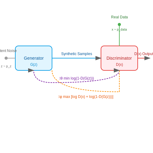
Generative Adversarial Networks (GANs) represent a breakthrough in unsupervised learning, framing the generative modeling problem as a two-player minimax game between competing neural networks. The fundamental architecture consists of:
- A generator (G) that learns to map latent noise vectors z to synthetic data samples
- A discriminator (D) that classifies inputs as real (from training data) or fake (from G)
The adversarial training objective can be formalized as:
where pdata is the real data distribution and pz is the latent noise distribution. The discriminator maximizes this value function by correctly identifying real and generated samples, while the generator minimizes it by fooling the discriminator.
Training Dynamics
The Nash equilibrium occurs when G perfectly replicates the data distribution (pg = pdata) and D outputs 0.5 everywhere (random guessing). In practice, training involves alternating gradient updates:
- Fix G and update D to maximize V(D,G)
- Fix D and update G to minimize V(D,G)
The gradients flow through both networks via backpropagation, with the generator's gradients coming from the discriminator's mistakes. This creates a delicate balance - if D becomes too strong too quickly, G receives uninformative gradients (the vanishing gradient problem).
Architectural Innovations
Several key innovations enable stable GAN training:
- Non-saturating loss: Modifies the generator objective to maximize log D(G(z)) rather than minimize log(1-D(G(z)))
- Batch normalization: Helps prevent mode collapse by decorrelating gradients across samples
- LeakyReLU activations: Mitigate the dying ReLU problem in discriminators
The theoretical framework builds on concepts from game theory, information geometry, and density ratio estimation. The discriminator implicitly estimates the ratio pdata(x)/pg(x) without explicitly modeling either distribution.
Challenges and Solutions
Common failure modes include:
- Mode collapse: Generator produces limited varieties of samples
- Oscillations: Networks fail to converge due to competing objectives
- Vanishing gradients: Poor discriminator feedback stalls generator learning
Modern solutions employ techniques like spectral normalization, gradient penalty, and progressive growing of networks. The Wasserstein GAN formulation replaces the original Jensen-Shannon divergence minimization with Earth Mover's distance, providing more stable training signals.
Key Innovations in Deep Convolutional GANs (DCGANs)
Architectural Improvements
The DCGAN architecture introduced several critical modifications to the traditional GAN framework that stabilized training and improved generation quality. First, it replaced deterministic spatial pooling functions (e.g., max pooling) with strided convolutions in the discriminator and fractional-strided convolutions in the generator. This allows the network to learn its own spatial downsampling and upsampling functions. The generator's architecture follows:
where z is the latent vector sampled from a uniform distribution. Batch normalization is applied to all layers except the generator output and discriminator input, addressing internal covariate shift and preventing mode collapse.
Strided Convolution Formulation
The fractional-strided convolution (transposed convolution) operation in the generator can be mathematically described as:
where I is input size, O output size, S stride, K kernel size, and P padding. This enables precise control over the upsampling process. For example, a 4×4 input with stride 2, kernel 5, and padding 1 produces a 10×10 output:
Elimination of Fully Connected Layers
DCGANs removed all fully connected layers, using only convolutional operations. The discriminator ends with a convolution followed by a sigmoid, while the generator starts with a fully connected layer only to project the latent vector into the initial convolutional feature map. This change:
- Reduced parameter count by ~80% compared to FC-heavy GANs
- Improved spatial locality in learned features
- Enabled scale-invariant feature learning
LeakyReLU Activation
The discriminator employs LeakyReLU activations (α=0.2) instead of vanilla ReLU:
This prevents the "dying ReLU" problem in the discriminator, maintaining gradient flow even for negative inputs. The generator uses ReLU except for the output layer (tanh), matching the pixel value range.
Latent Space Interpolation
DCGANs demonstrated that the learned latent space Z captures meaningful semantic directions. Arithmetic in Z space produces semantically meaningful image transformations, suggesting the network learns a disentangled representation. For two latent vectors z1 and z2:
with α ∈ [0,1], producing smooth interpolations between generated samples.
Visualization of Filters
The DCGAN paper introduced techniques to visualize learned convolutional filters by:
- Identifying neurons that maximize activation for specific visual concepts
- Projecting activations back to pixel space via deconvolution
- Demonstrating that filters learn hierarchical features (edges → textures → objects)
This provided empirical evidence that GANs learn hierarchical representations similar to supervised CNNs.
Architectural Components of DCGANs
Generator Network
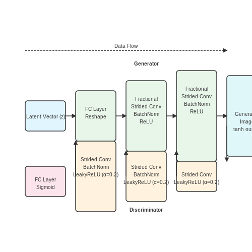
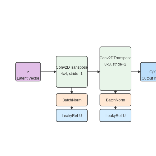
The generator in a DCGAN is a convolutional neural network (CNN) that transforms a latent noise vector z into a synthetic image. The architecture typically consists of transposed convolutional layers (also called fractionally strided convolutions), which progressively upsample the input noise into higher-resolution feature maps. Batch normalization and ReLU activations are applied after each transposed convolution, except for the final layer, which uses a tanh activation to constrain pixel values to [-1, 1].
where Wg represents the learned weights of the generator and bg the biases. The transposed convolution operation can be expressed as:
where x is the input feature map and y the upsampled output.
Discriminator Network
The discriminator is a CNN that classifies input images as real or fake. Unlike traditional CNNs, it uses strided convolutions instead of pooling layers for downsampling. LeakyReLU activations (with a slope of 0.2 for negative inputs) prevent vanishing gradients, while batch normalization stabilizes training. The final layer uses a sigmoid activation to output a probability score.
The discriminator's loss function combines binary cross-entropy for real and generated samples:
Key Architectural Innovations
- Removal of fully connected layers: Replaced with deep convolutional networks, enabling more stable training and higher-resolution image generation.
- Batch normalization: Applied to both generator and discriminator to mitigate internal covariate shift and prevent mode collapse.
- LeakyReLU in discriminator: Addresses dying ReLU problem by allowing small negative activations.
- Adam optimizer: Typically used with a learning rate of 0.0002 and momentum term β1 = 0.5 for stable training.
Layer Configuration Example
A common DCGAN generator architecture for 64×64 RGB images:
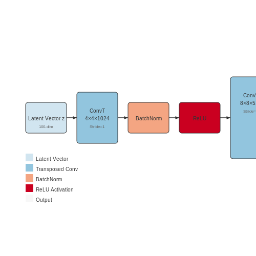
- Dense layer: Project 100-dim noise vector to 4×4×1024 feature map
- Transposed conv: 5×5 kernel, stride 2, output 8×8×512
- Transposed conv: 5×5 kernel, stride 2, output 16×16×256
- Transposed conv: 5×5 kernel, stride 2, output 32×32×128
- Transposed conv: 5×5 kernel, stride 2, output 64×64×3 (tanh activation)
Practical Implementation Considerations
When implementing DCGANs:
- Generator outputs should be normalized to match the training data distribution (typically [-1, 1] for tanh)
- Discriminator inputs should be preprocessed identically to real training images
- Weight initialization follows a normal distribution with mean 0 and standard deviation 0.02
- Label smoothing (using 0.9 instead of 1.0 for real images) can improve stability
2. Designing the Generator Network
Designing the Generator Network
The generator in a DCGAN transforms a latent noise vector z into a synthetic image. Unlike traditional GANs, DCGANs employ transposed convolutional layers (also called fractionally strided convolutions) to progressively upsample the input noise into higher-resolution feature maps. The architecture must balance two competing objectives: generating realistic images while remaining stable during adversarial training.
Architecture Components
The DCGAN generator consists of:
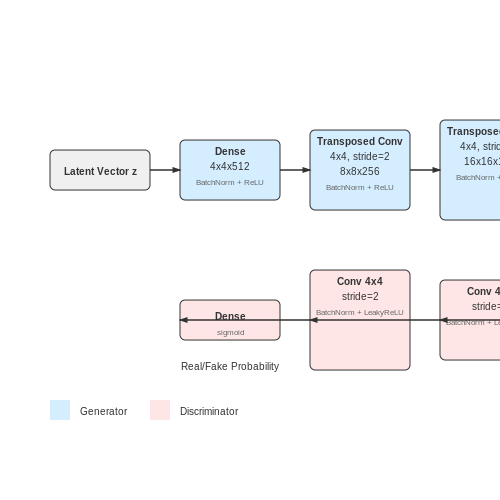
- Input Layer: A fully connected layer that projects the latent vector z into an initial feature volume. For example, a 100-dimensional noise vector might be reshaped into a 4x4x1024 tensor.
- Transposed Convolutional Blocks: Each block upsamples the spatial dimensions while reducing channel depth. A typical sequence progresses from 4x4 to 8x8, 16x16, 32x32, and finally 64x64 resolution.
- Batch Normalization: Applied after each transposed convolution to stabilize training by normalizing activations. This prevents mode collapse and accelerates convergence.
- Activation Functions: ReLU is used in hidden layers for non-linearity, while the output layer employs tanh to constrain pixel values to [-1, 1], matching normalized input data ranges.
Mathematical Formulation
The generator G maps latent noise z to an image x through a series of transposed convolutions. Each layer performs:
where fl is the activation function, Wl the learnable filters, and ∗T denotes transposed convolution. The upsampling factor is controlled by stride s:
where k is kernel size and p is padding.
Design Considerations
Key hyperparameters include:
- Latent Space Dimensionality: Higher dimensions (e.g., 100-512) capture more complex distributions but increase computational cost.
- Filter Count Progression: Common patterns include halving channels at each upsampling step (e.g., 1024 → 512 → 256 → 128 → 3).
- Kernel Sizes: 4x4 or 5x5 filters balance receptive field size and computational efficiency.
- Strides: Stride-2 upsampling doubles spatial dimensions while maintaining connectivity patterns.
Implementation Example
import torch.nn as nn

class Generator(nn.Module):
    def __init__(self, latent_dim=100, img_channels=3):
        super().__init__()
        self.main = nn.Sequential(
            # Input: latent_dim x 1 x 1
            nn.ConvTranspose2d(latent_dim, 1024, 4, 1, 0, bias=False),
            nn.BatchNorm2d(1024),
            nn.ReLU(True),
            # 1024 x 4 x 4
            nn.ConvTranspose2d(1024, 512, 4, 2, 1, bias=False),
            nn.BatchNorm2d(512),
            nn.ReLU(True),
            # 512 x 8 x 8
            nn.ConvTranspose2d(512, 256, 4, 2, 1, bias=False),
            nn.BatchNorm2d(256),
            nn.ReLU(True),
            # 256 x 16 x 16
            nn.ConvTranspose2d(256, img_channels, 4, 2, 1, bias=False),
            nn.Tanh()
            # 3 x 64 x 64
        )

    def forward(self, z):
        return self.main(z)
This architecture demonstrates the canonical DCGAN design pattern: progressive upsampling through strided transposed convolutions, batch normalization for stability, and ReLU/tanh activations for non-linearity and output scaling.
Designing the Discriminator Network
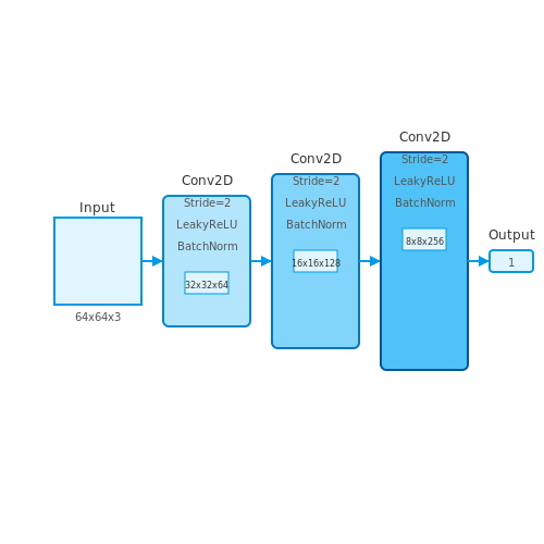
The discriminator in a DCGAN is a convolutional neural network (CNN) that classifies whether an input image is real (from the training dataset) or fake (generated by the generator). Its architecture is designed to progressively downsample spatial dimensions while increasing feature depth, enabling hierarchical feature extraction.
Architecture Components
The discriminator consists of several key layers:
- Input Layer: Accepts an image tensor of shape (batch_size, height, width, channels). For standard DCGANs, this is typically 64x64 or 128x128 RGB images.
- Convolutional Blocks: Each block contains:
- A 2D convolution with stride 2 (downsampling)
- Batch normalization (except the first layer)
- LeakyReLU activation (α=0.2)
- Final Layers: A dense layer with sigmoid activation outputs a single probability score.
Mathematical Formulation
The discriminator D(x) outputs the probability that input x is real. For a batch of images, the loss function is:
where G(z) is the generator's output. The discriminator is trained to maximize this objective, while the generator aims to minimize it.
Design Considerations
Key architectural choices include:
- Kernel Size: 5x5 or 4x4 convolutions balance receptive field and computational cost.
- Strides: Stride-2 convolutions reduce spatial dimensions by half each layer.
- Feature Maps: Start with 64 filters, doubling each layer (e.g., 64→128→256→512).
- Normalization: Batch norm stabilizes training but is omitted from the input layer.
Implementation Example
def build_discriminator(input_shape=(64, 64, 3)):
    model = Sequential()

    # First conv block (no batch norm)
    model.add(Conv2D(64, kernel_size=4, strides=2,
                    padding='same', input_shape=input_shape))
    model.add(LeakyReLU(alpha=0.2))

    # Subsequent blocks
    for filters in [128, 256, 512]:
        model.add(Conv2D(filters, kernel_size=4, strides=2, padding='same'))
        model.add(BatchNormalization())
        model.add(LeakyReLU(alpha=0.2))

    # Output layer
    model.add(Flatten())
    model.add(Dense(1, activation='sigmoid'))

    return model
Performance Optimization
To improve discriminator effectiveness:
- Label Smoothing: Replace hard 0/1 labels with 0.1/0.9 to reduce overconfidence.
- Gradient Penalty: Used in WGAN-GP to enforce Lipschitz continuity.
- Spectral Normalization: Constrains layer weights to stabilize training.
2.3 Loss Functions and Training Dynamics
Adversarial Loss Formulation
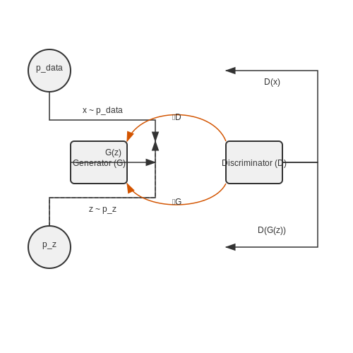
The core training mechanism of a DCGAN relies on a minimax game between the generator G and the discriminator D, formalized by the adversarial loss function. The objective function V(G, D) is derived from the binary cross-entropy loss, where D aims to maximize the probability of correctly classifying real and fake samples, while G aims to minimize the probability that D correctly identifies its outputs as fake.
Here, x represents real data samples drawn from the true distribution pdata(x), while z is a noise vector sampled from a prior distribution pz(z) (typically Gaussian or uniform). The discriminator outputs a probability D(x) that x is real, and D(G(z)) is the probability that the generated sample G(z) is real.
Training Dynamics and Mode Collapse
Training DCGANs involves alternating gradient updates for D and G. In practice, D is trained for k steps (often k=1) before updating G to prevent the discriminator from becoming too strong. However, this leads to several challenges:
- Vanishing Gradients: If D becomes too confident, log(1 - D(G(z))) saturates, providing negligible gradients for G.
- Mode Collapse: G may collapse to producing a limited set of outputs, failing to capture the full data distribution.
To mitigate these issues, the generator is often trained to maximize log(D(G(z))) instead of minimizing log(1 - D(G(z))), providing stronger gradients early in training.
Non-Saturating Loss and Practical Modifications
The non-saturating heuristic modifies the generator's loss to avoid gradient saturation:
Meanwhile, the discriminator's loss remains unchanged. Additional stabilization techniques include:
- Label Smoothing: Replacing hard labels (0 for fake, 1 for real) with soft targets (e.g., 0.1 and 0.9) to reduce discriminator overconfidence.
- Instance Noise: Adding Gaussian noise to discriminator inputs to prevent overfitting.
- Feature Matching: Forcing G to match intermediate feature statistics of real data in the discriminator.
Convergence Metrics and Stability
Monitoring DCGAN training requires careful evaluation beyond loss values, as they may not correlate with sample quality. Common metrics include:
- Inception Score (IS): Measures diversity and quality by evaluating classifier predictions on generated images.
- Fréchet Inception Distance (FID): Compares feature distributions of real and generated images in a pretrained network.
Training stability can be improved using spectral normalization in D and batch normalization in G, ensuring Lipschitz continuity and preventing gradient explosion.
3. Data Preparation and Augmentation
3.1 Data Preparation and Augmentation
Training a DCGAN requires high-quality, preprocessed image data to ensure stable convergence and realistic output. The data pipeline must address normalization, augmentation, and batch construction to optimize the adversarial training process.
Normalization and Scaling
Pixel values in input images are typically scaled to the range [-1, 1] to match the output range of the generator's tanh activation function. For an image tensor X with pixel values in [0, 255], normalization is applied as:
This scaling ensures zero-centered inputs, improving gradient flow during backpropagation. Batch normalization layers in both the generator and discriminator further stabilize training by maintaining consistent feature distributions.
Data Augmentation Strategies
Augmentation artificially expands the training dataset by applying random transformations, reducing overfitting and improving generalization. Common techniques include:
- Random horizontal flipping: Preserves spatial semantics while doubling effective dataset size.
- Small-angle rotations (±5°): Introduces viewpoint variation without distorting objects.
- Color jitter: Adjusts brightness, contrast, and saturation within bounded ranges to simulate lighting variations.
For high-resolution datasets, geometric augmentations (e.g., scaling, cropping) must be applied carefully to avoid introducing artifacts that the discriminator could exploit as false signals.
Batch Construction and Shuffling
Mini-batch diversity is critical for GAN training. Each batch should contain randomly sampled images to prevent mode collapse. The batch size B is typically a power of 2 (e.g., 64, 128) to align with GPU memory optimizations. A shuffled dataset iterator ensures stochastic gradient updates follow the form:
where θ represents the discriminator's parameters, x_i are real images, and z_i are latent vectors.
Dataset-Specific Considerations
For class-conditional DCGANs, label information must be embedded as one-hot vectors concatenated with the latent space. Datasets like CIFAR-10 or ImageNet require:
- Resolution matching: All images resized to a fixed dimension (e.g., 64×64 or 128×128) using Lanczos interpolation.
- Channel alignment: Conversion to RGB format, even for grayscale sources, to maintain consistent tensor shapes.
Preprocessing pipelines should be implemented efficiently using GPU-accelerated libraries like TensorFlow's tf.data or PyTorch's DataLoader to minimize I/O bottlenecks.
Handling Imbalanced Data
When training on datasets with class imbalances, stratified sampling or weighted loss functions prevent the generator from favoring majority classes. The discriminator's loss can be modified as:
where w_y is the inverse class frequency for sample x with label y.
3.2 Hyperparameter Tuning and Optimization
The performance of a Deep Convolutional Generative Adversarial Network (DCGAN) is highly sensitive to hyperparameter choices. Unlike traditional deep learning models, DCGANs involve a dynamic equilibrium between the generator (G) and discriminator (D), making hyperparameter tuning critical for stable training and high-quality image synthesis.
Learning Rates and Optimizer Selection
The learning rates for G and D must be carefully balanced to prevent one network from overpowering the other. Empirical studies suggest using a lower learning rate for G (typically 1e-4 to 2e-4) compared to D (2e-4 to 5e-4). Adam optimizer is preferred due to its adaptive momentum properties, with recommended hyperparameters:
Lower β1 helps mitigate mode collapse by reducing the influence of past gradients. The discriminator is often trained k times (where k ∈ [1,5]) per generator update to maintain equilibrium.
Batch Normalization and Layer Configurations
Batch normalization (BN) stabilizes training by normalizing layer inputs, but its application must be strategic:
- Apply BN in all layers of G except the output layer.
- Avoid BN in the discriminator’s input layer to prevent artifacts.
- Use LeakyReLU (α=0.2) in D for sparse gradients, while G employs ReLU for smoother feature propagation.
Spectral normalization can further stabilize D by constraining its Lipschitz constant, replacing BN in some architectures.
Noise Vector Sampling and Dimensionality
The latent vector z is sampled from a normal distribution N(0,I), but dimensionality impacts output diversity:
Higher d (e.g., 128–512) improves feature disentanglement but requires deeper networks. Truncation tricks—clamping z to ±2σ—can trade diversity for fidelity during inference.
Loss Functions and Gradient Penalties
Wasserstein loss with gradient penalty (WGAN-GP) often outperforms standard GAN loss by enforcing Lipschitz continuity:
Here, λ (typically 10) controls penalty strength, and ẑ is sampled from interpolated real-fake data pairs. This mitigates vanishing gradients and mode collapse.
Architectural Tweaks for High-Resolution Outputs
For resolutions ≥128×128, progressive growing—gradually increasing layer depth—avoids memory bottlenecks. Key adjustments:
- Use pixel-wise feature normalization in G to prevent magnitude explosion.
- Replace transpose convolutions with bilinear upsampling + convolution to reduce checkerboard artifacts.
- Balance network width (e.g., 64–512 filters) relative to dataset complexity.
Training dynamics can be monitored via the Frechet Inception Distance (FID), where lower values indicate better realism and diversity:
Here, (μr, Σr) and (μg, Σg) are feature statistics of real and generated images from an Inception-v3 network.
3.3 Common Challenges and Mitigation Strategies
Mode Collapse
Mode collapse occurs when the generator produces a limited variety of samples, often converging to a few modes of the data distribution. This happens because the generator finds a small set of outputs that reliably fool the discriminator, leading to repetitive or low-diversity generations. Mathematically, this can be understood as the generator optimizing for a subset of the data distribution:
When mode collapse occurs, the generator effectively minimizes the second term by producing a small set of outputs that maximize \(D(G(z))\). To mitigate this:
- Mini-batch discrimination: The discriminator evaluates samples in batches, comparing statistical features across the batch to detect lack of diversity.
- Unrolled GANs: The generator’s optimization considers multiple future steps of the discriminator, preventing short-term exploitation.
- Feature matching: The generator is trained to match the statistics (e.g., mean, variance) of real data features in an intermediate layer of the discriminator.
Training Instability
DCGANs are prone to training instability due to the adversarial nature of the loss landscape. The discriminator can become too strong, providing no meaningful gradient for the generator, or vice versa. This is reflected in the vanishing gradients problem:
Strategies to stabilize training include:
- Label smoothing: Replace hard labels (0 for fake, 1 for real) with soft targets (e.g., 0.1 and 0.9) to prevent overconfident discriminator predictions.
- Gradient penalty: Enforce Lipschitz continuity on the discriminator via a gradient penalty term, as in Wasserstein GANs (WGAN-GP):
Poor Image Quality
Generated images may suffer from artifacts, blurriness, or unrealistic textures. This often stems from:
- Architectural limitations: Inadequate receptive fields or channel dimensions in the generator.
- Loss function misalignment: Traditional GAN losses (e.g., binary cross-entropy) may not correlate well with perceptual quality.
Solutions include:
- Progressive growing: Start training with low-resolution images and gradually increase resolution, as in ProGAN.
- Perceptual loss: Augment the adversarial loss with a feature-based loss (e.g., VGG network activations) to improve texture realism.
Hyperparameter Sensitivity
DCGANs are highly sensitive to hyperparameters such as learning rates, batch sizes, and optimizer choices. For instance:
- Learning rate imbalance: A discriminator learning rate too high can overpower the generator.
- Batch normalization: Incorrect use (e.g., applying it to the generator’s output layer) can lead to artifacts.
Best practices include:
- Using Adam optimizer with \( \beta_1 = 0.5 \) and \( \beta_2 = 0.999 \).
- Setting equal learning rates for generator and discriminator (e.g., \( 2 \times 10^{-4} \)).
Evaluation Challenges
Quantifying DCGAN performance is non-trivial. Common pitfalls include:
- Inception Score (IS): Favors high-class discriminability but ignores intra-class diversity.
- Frechet Inception Distance (FID): More robust but computationally expensive.
Practical workarounds:
- Track multiple metrics (IS, FID, precision/recall for generative models).
- Use human evaluation for critical applications.
4. Quantitative Metrics for Image Generation
4.1 Quantitative Metrics for Image Generation
Evaluating the quality of generated images in DCGANs requires objective, quantitative metrics beyond subjective visual inspection. Three widely adopted metrics are the Inception Score (IS), Fréchet Inception Distance (FID), and Precision-Recall for Generative Models (PR). Each measures different aspects of image quality, diversity, and realism.
Inception Score (IS)
The Inception Score quantifies both the quality and diversity of generated images by leveraging a pre-trained Inception-v3 network. It is defined as:
where \( p(y|x) \) is the conditional class distribution for image \( x \), and \( p(y) = \int p(y|x) p_g(x) dx \) is the marginal class distribution over generated images \( p_g \). Higher IS values indicate better performance, as they reflect high-confidence predictions (quality) and diverse class coverage (diversity).
Fréchet Inception Distance (FID)
FID compares the statistics of generated and real images in the feature space of Inception-v3. Given real images \( X \) and generated images \( Y \), with feature means \( \mu_r, \mu_g \) and covariance matrices \( \Sigma_r, \Sigma_g \), FID is computed as:
Lower FID scores indicate closer similarity between generated and real images. Unlike IS, FID accounts for feature-level similarity rather than just class distributions.
Precision-Recall for Generative Models (PR)
PR metrics decompose FID into two components: precision (quality of generated samples) and recall (coverage of real data distribution). Given manifolds \( S_g \) (generated) and \( S_r \) (real):
where \( d(\cdot, \cdot) \) is a distance metric (e.g., Euclidean in feature space) and \( \epsilon \) is a threshold. PR curves provide a nuanced view of the trade-off between sample quality and diversity.
Practical Considerations
- Computational Cost: FID requires calculating covariance matrices, which can be expensive for large datasets.
- Sensitivity to Noise: IS can be artificially inflated by adversarial examples that maximize classifier confidence.
- Dataset Bias: All metrics depend on the Inception-v3 network trained on ImageNet, which may not generalize to niche domains.
4.2 Qualitative Assessment Techniques
Qualitative assessment of DCGAN-generated images relies on human visual inspection to evaluate perceptual quality, diversity, and coherence. Unlike quantitative metrics, which provide scalar scores, qualitative analysis captures nuanced aspects of image generation that are difficult to quantify mathematically.
Visual Fidelity Metrics
Generated images should exhibit high visual fidelity, meaning they must resemble real-world samples from the training distribution. Key indicators include:
- Sharpness: Absence of blurry or overly smooth regions.
- Texture Detail: Presence of fine-grained textures (e.g., fabric patterns, skin pores).
- Structural Coherence: Logical arrangement of object parts (e.g., correct facial feature placement).
Artifacts like checkerboard patterns or ghosting effects often emerge from unstable training or improper upsampling in the generator.
Diversity Assessment
A well-trained DCGAN should produce diverse outputs across different latent space samples. Practitioners evaluate this by:
- Sampling multiple latent vectors and verifying distinct outputs.
- Checking for mode collapse, where the generator produces nearly identical images regardless of input noise.
Interpolating between latent vectors should yield smooth transitions between semantically meaningful features.
Semantic Validity
Generated content must adhere to domain-specific constraints. For facial generation, this includes:
- Symmetrical eye placement
- Physically plausible lighting/shadow interactions
- Consistent color palettes
Failure modes often manifest as impossible geometries (e.g., ears growing from foreheads) or surreal combinations of features.
Comparative Evaluation
Side-by-side comparisons with real images from the training set reveal:
Where \(G(z_i)\) denotes generated images and \(x_i\) represents real samples. While this resembles a quantitative metric, practitioners primarily use it for visual benchmarking.
Failure Mode Analysis
Common DCGAN failure patterns include:
- Mode Dropping: Ignoring minority classes in imbalanced datasets
- High-Frequency Artifacts: Grid-like patterns from transposed convolutions
- Semantic Entanglement: Inseparable feature correlations (e.g., always generating glasses with beards)
Progressive growing techniques and spectral normalization often mitigate these issues.
4.3 Comparing DCGANs with Other Generative Models
DCGANs (Deep Convolutional Generative Adversarial Networks) represent a specialized variant of GANs optimized for image generation, but they are not the only generative model available. Understanding their strengths and weaknesses relative to other approaches—such as Variational Autoencoders (VAEs), Flow-based models, and autoregressive models—is critical for selecting the right architecture for a given task.
DCGANs vs. Variational Autoencoders (VAEs)
VAEs employ an encoder-decoder architecture, learning a probabilistic latent space by optimizing a lower bound on the data likelihood. The key distinction lies in their training objective: VAEs minimize the Kullback-Leibler (KL) divergence between the learned latent distribution and a prior (typically Gaussian), whereas DCGANs rely on adversarial training to match generated and real data distributions.
DCGANs often produce sharper images than VAEs due to their adversarial loss, but VAEs offer better interpretability of latent space and more stable training. VAEs also excel at tasks requiring probabilistic inference, such as anomaly detection, while DCGANs are better suited for high-fidelity image synthesis.
DCGANs vs. Flow-Based Models
Flow-based models, such as Glow or RealNVP, use invertible transformations to map data to a latent space with exact likelihood computation. Unlike DCGANs, which lack an explicit likelihood model, flow-based models optimize the exact log-likelihood:
While flow-based models provide tractable likelihoods and exact sampling, they are computationally expensive due to the requirement of invertible transformations. DCGANs, in contrast, are more scalable for high-resolution image generation but lack explicit density estimation.
DCGANs vs. Autoregressive Models
Autoregressive models, like PixelRNN or PixelCNN, generate images sequentially by modeling the conditional distribution of each pixel given previous pixels. Their likelihood-based training ensures stable convergence, but their sequential nature makes them slower than DCGANs for parallel generation. DCGANs, with their adversarial framework, can generate entire images in a single forward pass, making them more efficient for real-time applications.
Practical Trade-offs
- Training Stability: VAEs and autoregressive models are more stable but may produce blurrier outputs compared to DCGANs.
- Sample Quality: DCGANs and flow-based models generate sharper images, but flow-based models require significant computational resources.
- Latent Space Control: VAEs and flow-based models offer better interpolation and manipulation in latent space, whereas DCGANs require additional techniques (e.g., latent space regularization) for meaningful control.
Recent hybrid approaches, such as VQ-VAE (Vector Quantized Variational Autoencoder) and diffusion models, combine elements of these architectures, offering improved sample quality and training stability. However, DCGANs remain a popular choice for tasks where adversarial training’s benefits outweigh its instability.
5. Image Synthesis and Super-Resolution
DCGANs for Image Synthesis and Super-Resolution
Architecture and Training Dynamics
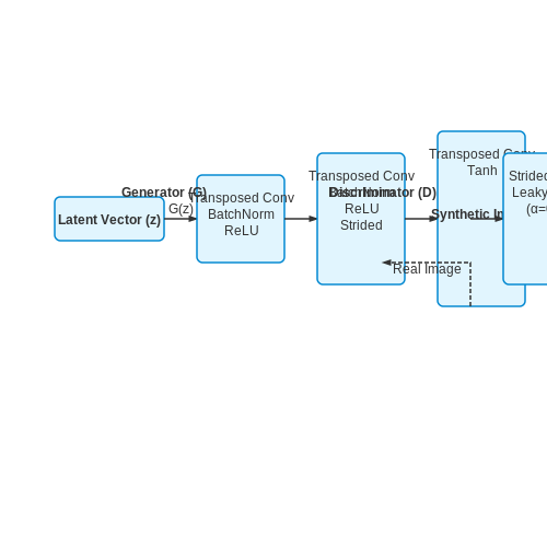
Deep Convolutional Generative Adversarial Networks (DCGANs) extend traditional GANs by leveraging convolutional layers without pooling, replacing them with strided convolutions for downsampling and transposed convolutions for upsampling. The generator G maps a latent vector z to an image space, while the discriminator D classifies real vs. synthetic images. The adversarial loss is defined as:
Batch normalization stabilizes training by normalizing activations across mini-batches, preventing mode collapse. LeakyReLU (α=0.2) in D avoids sparse gradients, while ReLU in G ensures non-linearity. The absence of fully connected layers enhances spatial coherence in generated images.
Super-Resolution via DCGANs
For super-resolution, DCGANs employ a modified generator that upsamples low-resolution (LR) inputs. The loss function combines adversarial loss with a pixel-wise L1 term to preserve structural fidelity:
Here, x is the LR image, y the high-resolution (HR) target, and λadv, λL1 balance adversarial sharpness and pixel accuracy. Transposed convolutions in G are often replaced with sub-pixel convolution layers to reduce checkerboard artifacts.
Practical Applications and Limitations
- Medical Imaging: DCGANs synthesize high-resolution MRI scans from low-quality inputs, aiding diagnosis where HR data is scarce.
- Satellite Imagery: Enhances spatial resolution of aerial photos by 4×, critical for environmental monitoring.
- Art Restoration: Reconstructs damaged artworks by inferring missing details from partial inputs.
However, DCGANs struggle with high-frequency details in extreme super-resolution (8×+), often producing blurred edges. Progressive growing of GANs (PGGANs) and attention mechanisms are later advancements addressing this.
Mathematical Derivation: Gradient Updates
The discriminator’s gradient w.r.t. its parameters θD is derived via backpropagation:
For the generator, the gradient avoids saturation by maximizing D(G(z)) instead of minimizing log(1 - D(G(z))):
This update rule mitigates vanishing gradients early in training when D confidently rejects synthetic samples.
5.2 Data Augmentation for Training Sets
Training deep convolutional generative adversarial networks (DCGANs) requires large, diverse datasets to prevent mode collapse and ensure high-quality image synthesis. However, acquiring extensive labeled datasets is often impractical. Data augmentation artificially expands the training set by applying label-preserving transformations to existing samples, improving generalization and robustness. For DCGANs, augmentation must maintain the statistical properties of the original distribution while introducing meaningful variability.
Common Augmentation Techniques
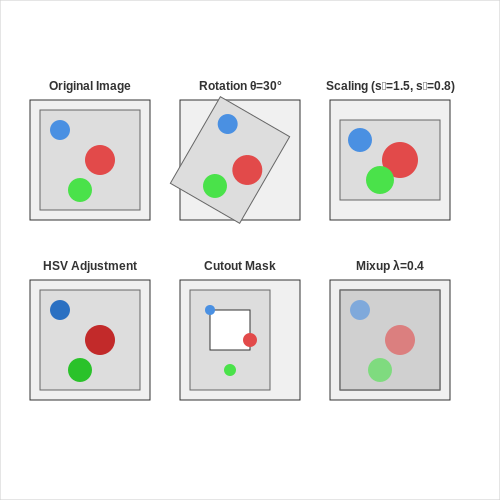
Geometric transformations such as rotation, scaling, and flipping are widely used due to their simplicity and effectiveness. Given an input image I with height H and width W, a random affine transformation can be represented as:
where sx, sy are scaling factors, θ is the rotation angle, and tx, ty are translation offsets. Bilinear interpolation ensures smooth pixel sampling during transformation.
Photometric Augmentations
Color space manipulations introduce variability in lighting and contrast without altering semantic content. For RGB images, channel-wise adjustments can be modeled as:
where α controls contrast, β adjusts brightness, and 𝒩 adds Gaussian noise with variance σ2. Hue-saturation-value (HSV) augmentations often yield more natural variations than direct RGB modifications.
Advanced Techniques
Cutout and mixup regularization methods have proven particularly effective for DCGAN training:
- Cutout randomly masks rectangular regions of the input image, forcing the generator to learn distributed representations.
- Mixup creates convex combinations of image pairs and their labels: Imix = λIi + (1-λ)Ij, where λ ∼ Beta(α,α).
Diffusion-based augmentation, which applies controlled noise injection through learned forward processes, has shown promise in recent studies. This approach maintains semantic consistency while exploring the data manifold more effectively than traditional methods.
Implementation Considerations
Augmentation pipelines must balance diversity and realism. Excessive transformations can introduce artifacts that degrade sample quality. Best practices include:
- Applying augmentations on-the-fly during training to minimize memory overhead
- Using differentiable operations when training GANs end-to-end
- Monitoring the Fréchet Inception Distance (FID) to assess augmentation impact
The augmentation policy should be adapted to the dataset characteristics. For example, medical imaging requires more constrained transformations than natural scenes to preserve diagnostic features.
Creative Applications in Art and Design
Deep Convolutional Generative Adversarial Networks (DCGANs) have revolutionized digital art and design by enabling the synthesis of high-resolution, photorealistic images from random noise vectors. The generator architecture, typically composed of transposed convolutional layers, learns to map latent space vectors z to output images G(z) that mimic the training distribution. The discriminator D provides adversarial feedback, forcing G to produce increasingly convincing artifacts.
Style Transfer and Hybridization
DCGANs excel at blending artistic styles by conditioning the generator on multiple input domains. For instance, a single model can be trained on both Renaissance paintings and modern abstract art, allowing interpolation in latent space to produce novel hybrid styles. The loss function for such multi-modal generation extends the standard DCGAN objective:
where λ controls the strength of the style preservation term Lstyle, often implemented using Gram matrix matching from convolutional feature activations.
Procedural Content Generation
Game designers leverage DCGANs to create infinite variations of textures, characters, and environments. The key innovation lies in the disentanglement of latent variables - modifying individual dimensions of z produces interpretable changes in output features. For example, in a character generation system:
- Latent dimension 1-3 control body proportions
- Dimensions 4-6 govern color palette
- Dimensions 7-9 influence armor style
This controllability emerges from the generator's hierarchical architecture, where early layers determine broad structural features while deeper layers refine fine details.
Architectural Design Exploration
DCGANs assist architects in rapidly generating building facade variations by learning from historical design corpora. The 3D-consistent nature of the outputs stems from the generator's spatial awareness, achieved through:
- Fractionally-strided convolutions maintaining spatial relationships
- Batch normalization stabilizing gradient flow
- LeakyReLU activations preserving low-level features
When trained on parametric CAD models, the generator learns to output construction-ready designs with proper topological constraints. The adversarial training ensures generated structures respect physical plausibility boundaries learned from the training set.
Fashion and Textile Design
High-end fashion houses employ DCGANs to create never-before-seen fabric patterns and garment designs. The generator's ability to combine learned features in novel ways produces commercially viable designs at scale. A critical enhancement involves conditioning the generator on textual descriptions:
where c represents a 300-dimensional embedding of the design brief (e.g., "floral silk evening gown with gold embroidery"). The discriminator simultaneously evaluates visual quality and semantic alignment.
Interactive Art Installations
Contemporary artists build DCGAN-powered installations that respond to viewer input in real-time. By implementing the generator in shader languages and optimizing for low-latency inference, these systems can:
- Transform visitor silhouettes into mythological creatures
- Generate infinite unique digital paintings based on ambient sound
- Create evolving abstract patterns driven by crowd movement
The technical challenge lies in distilling the DCGAN into a more compact network (e.g., using knowledge distillation) while preserving generation quality at interactive frame rates (>30fps).
6. Key Research Papers on DCGANs
6.1 Key Research Papers on DCGANs
- GANs and DCGANs for generation of topology optimization validation ... — The input values for the DCGANs are the optimized topology images, the compliance and M u. An appropriate activation function and optimizer are utilized in numerical example. The GANs and the DCGANs are alternately trained with 10,000 epochs. The total number of 3000 augmented data were obtained by the GANs and the DCGANs as shown in Fig. 6.
- Application of an Improved DCGAN for Image Generation — The remainder of the paper is organized as follows: Section 1 summarizes the progress of research with regard to GANs and the DCGAN; Section 2 mainly introduces the principles of the improved DCGAN algorithm and designs the network structure; Section 3 constructs the image generation models, with one based on GANs and the other based on the ...
- PDF Exploring Realistic Image Synthesis using Deep Convolutional GANs - IJRTI — DCGANs, a variant of GANs, leverage deep convolutional neural networks for image generation. These networks are characterized by the use of convolutional layers, which enable the model to learn intricate features and patterns from the input data. DCGANs have proven particularly effective in generating high-quality images by employing deep
- Augmentation of Images through DCGANs - IEEE Xplore — Now-a-days, extending images has become a challenging task to implement. Many of algorithms like convolution neural networks (CNN), Generative Adversarial Network (GAN) are used to fill out the image spaces. But the challenge arrives to guess or make appropriate assumption of image extended borders. We used Deep Convolution Generative Adversarial Network(DCGAN) over GAN and CNN to implement it ...
- PDF CMSC498L Final Project Report: Generative Adversarial Networks and ... — The authors trained DCGANs on three image datasets: Large-scale Scene Understanding (LSUN), Imagenet-1k, and a Faces dataset created by the authors. The generator of the model is able to transform a vector to a 64x64 pixel image by learning the representation of the dataset. 4 Our Implementation
- Exploring deep convolutional generative adversarial networks ... - Springer — Over the past few years, there has been a proliferation of research in the area of generative adversarial networks (GANs). GANs present a novel approach to producing synthetic data in varying fields including medicine, traffic control, text transferring, image generation, and cybersecurity. To improve the quality of synthetic generation, specifically for images, the GAN technique was paired ...
- (PDF) Application of an Improved DCGAN for Image Generation - ResearchGate — In this paper, based on a traditional generative adversarial networks (GANs) image generation model, first, the fully connected layer of the DCGAN is further improved.
- DCGAN: Deep Convolutional GAN with Attention Module for Remote View ... — In recent times, the development of Deep Learning Techniques for Image Classification has increased. The deep learning module uses an unsupervised learning technique. The supervised learning requires an adequate and outsized dataset with labels to train a machine. This paper proposes a unique Unsupervised Deep Feature Learning Method called Deep Convolutional GAN (DCGAN) with Attention Module ...
- DCGAN: Generate images with Deep Convolutional GAN — In the initializer __init__, an additional keyword argument models is required as you can see the code below. Also, we use keyword arguments iterator, optimizer and device.It should be noted that the optimizer augment takes a dictionary. The two different models require two different optimizers. To specify the different optimizers for the models, we give a dictionary, {'gen': opt_gen, 'dis ...
- (PDF) DCGAN--Image Generation - ResearchGate — This paper proposes an augmentation mechanism to improve the dataset's size, quality, and diversity using a set of different augmentations, namely flipping of images, rotations, shear, affine ...
6.2 Recommended Books and Tutorials
- Generative Adversarial Networks for Image Generation — Additionally, it explores three promising applications of GANs, including image-to-image translation, unsupervised domain adaptation and GANs for security. This book appeals to students and researchers who are interested in GANs, image generation and general machine learning and computer vision.
- 20.2. Deep Convolutional Generative Adversarial Networks - D2L — 20.2.2. The Generator The generator needs to map the noise variable z ∈ R d, a length- d vector, to a RGB image with width and height to be 64 × 64 . In Section 14.11 we introduced the fully convolutional network that uses transposed convolution layer (refer to Section 14.10) to enlarge input size.
- PDF Generative Adversarial Networks and Deep Learning: Theory and Applications — There are various applications of GAN in science and technology, including computer vision, security, ultimedia and advertisements, image generation and translation, text-to-images synthesis, video synthesis, high-resolution image generation, drug discovery, etc."- Provided by publisher.
- Generative Adversarial Networks for Image-to-Image Translation — Both of these networks contest with each other, similar to game theory. The generator is responsible for generating quality images that should resemble ground truth, and the discriminator is accountable for identifying whether the generated image is a real image or a fake image generated by the generator.
- DCGAN: Generate images with Deep Convolutional GAN — DCGAN: Generate images with Deep Convolutional GAN ¶ 0. Introduction ¶ In this tutorial, we generate images with generative adversarial networks (GAN). GAN are kinds of deep neural network for generative modeling that are often applied to image generation. GAN-based models are also used in PaintsChainer, an automatic colorization service.
- Image Generation using Generative Adversarial Networks (GANs) using ... — Training GANs for Image Generation Generative Adversarial Networks (GANs) consist of two neural networks—the Generator and the Discriminator—that compete with each other.
- (PDF) DCGAN--Image Generation - ResearchGate — Training modern generative adversarial networks (GANs) to produce high-quality images requires massive datasets, which are challenging to obtain in many real-world scenarios, like healthcare.
- Deep Convolutional Generative Adversarial Network - TensorFlow — This tutorial demonstrates how to generate images of handwritten digits using a Deep Convolutional Generative Adversarial Network (DCGAN). The code is written using the Keras Sequential API with a tf.GradientTape training loop. What are GANs? Generative Adversarial Networks (GANs) are one of the most interesting ideas in computer science today.
- 深度学习入门与Pytorch|6.2 DCGAN的介绍、代码与应用 - 知乎 — 上一节介绍了 GAN的基本实现方法,但在实际中很少会直接用最基本的版本。现在广泛使用的是深度卷积生成对抗网络——DCGAN。DCGAN是在GAN的基础上设计的架构,在训练过程中状态稳定,可以有效实现高质量的图片生成…
6.3 Open-Source Implementations and Tools
- Implementing DCGAN for Generating Images in Keras - Scaler — DCGANs have been used for various applications, such as image generation, image translation, and text-to-image synthesis. Consider exploring some of these applications and seeing how DCGANs can be used to solve them.
- GitHub - singh-priyanshi/DCGANs-for-Image-Generation — DCGANs offer a powerful way to model complex data distributions, particularly for generating realistic images. This project covers both theoretical and practical aspects of implementing DCGANs for two different types of datasets.
- Hybrid Deep Convolutional Generative Adversarial Networks (DCGANS) and ... — Generative Adversarial Networks or GANS, are another way of achieving generative modeling using various deep learning methods like convoluted neural networks. They have a wide range of applications like :- image to image translation, improving the resolution of the images, creating multiple images using a single image, checking if the image is real or fake and the list goes on. One of the ...
- Step-by-Step Guide for Creating a DCGAN Model - Analytics Vidhya — The generated images' quality improves with longer training times and on more powerful hardware. Experimenting with DCGANs opens up exciting possibilities for creative applications, such as generating art, creating virtual characters, and enhancing data augmentation for various machine-learning tasks.
- DCGAN: Generate images with Deep Convolutional GAN — DCGAN: Generate images with Deep Convolutional GAN ¶ 0. Introduction ¶ In this tutorial, we generate images with generative adversarial networks (GAN). GAN are kinds of deep neural network for generative modeling that are often applied to image generation. GAN-based models are also used in PaintsChainer, an automatic colorization service. In this tutorial, you will learn the following things ...
- Application of an Improved DCGAN for Image Generation — A deep convolutional generative adversarial network (DCGAN) can better adapt to complex image distributions than other methods. In this paper, based on a traditional generative adversarial networks (GANs) image generation model, first, the fully connected layer of the DCGAN is further improved.
- 20.2. Deep Convolutional Generative Adversarial Networks - D2L — 20.2.2. The Generator The generator needs to map the noise variable z ∈ R d, a length- d vector, to a RGB image with width and height to be 64 × 64 . In Section 14.11 we introduced the fully convolutional network that uses transposed convolution layer (refer to Section 14.10) to enlarge input size.
- Exploring deep convolutional generative adversarial networks ... - Springer — To improve the quality of synthetic generation, specifically for images, the GAN technique was paired with convolutional neural networks (CNNs) to build deep convolutional generative adversarial networks (DCGAN). The DCGAN framework is a simple yet stable framework shown to generate quality photorealistic images.
- (PDF) DCGAN--Image Generation - ResearchGate — Training modern generative adversarial networks (GANs) to produce high-quality images requires massive datasets, which are challenging to obtain in many real-world scenarios, like healthcare.
- Deep Convolutional Generative Adversarial Network - TensorFlow — This tutorial demonstrates how to generate images of handwritten digits using a Deep Convolutional Generative Adversarial Network (DCGAN). The code is written using the Keras Sequential API with a tf.GradientTape training loop. What are GANs? Generative Adversarial Networks (GANs) are one of the most interesting ideas in computer science today. Two models are trained simultaneously by an ...