

Denoising Score Matching Explained
1. What is Score Matching?
What is Score Matching?
Score matching is a technique for estimating the gradient of the log-probability density function (the score function) of a data distribution without explicitly modeling the density itself. Given a dataset sampled from an unknown distribution pdata(x), the goal is to learn a model sθ(x) that approximates the true score ∇x log pdata(x).
Mathematical Foundation
The score function is defined as the gradient of the log-density with respect to the data:
Score matching avoids the intractable partition function in density estimation by directly optimizing the model to match the score function. The objective minimizes the expected squared difference between the model and the true score:
However, since ∇x log pdata(x) is unknown, score matching derives an equivalent objective that depends only on the model and its derivatives:
Practical Implications
This formulation bypasses the need for adversarial training (as in GANs) or variational bounds (as in VAEs). It is particularly useful for:
- Generative modeling: Enables sampling via Langevin dynamics, where samples are generated by iteratively following the score.
- Denoising: The score provides the direction to "denoise" corrupted data points.
- Manifold learning: The score captures the local structure of the data distribution.
Connection to Denoising Score Matching
In high-dimensional spaces, the trace term tr(∇x sθ(x)) becomes computationally expensive. Denoising score matching (DSM) circumvents this by perturbing data with noise and learning the score of the perturbed distribution:
Here, q(ẋ|x) is a predefined noise distribution (e.g., Gaussian). DSM is equivalent to the original score matching objective when the noise is sufficiently small.
The Role of Noise in Score Estimation
Noise plays a fundamental role in denoising score matching by enabling the estimation of the score function—the gradient of the log-probability density—without explicit knowledge of the true data distribution. The key insight is that perturbing data with carefully controlled noise simplifies the learning objective while preserving the underlying structure of the data manifold.
Noise as a Regularizer
Adding isotropic Gaussian noise to the data smooths the probability density function, making the score function easier to estimate. For a noise variance σ², the perturbed data distribution qσ(x̃|x) is given by:
This noise-induced smoothing ensures the score ∇x̃ log qσ(x̃) is well-defined even when the true data distribution pdata(x) is degenerate or supported on a low-dimensional manifold. The noise level σ acts as a hyperparameter balancing fidelity to the original data against the smoothness of the learned score.
Noise-Controlled Score Matching Objective
The denoising score matching objective minimizes the expected difference between the model's score and the score of the noise-perturbed distribution:
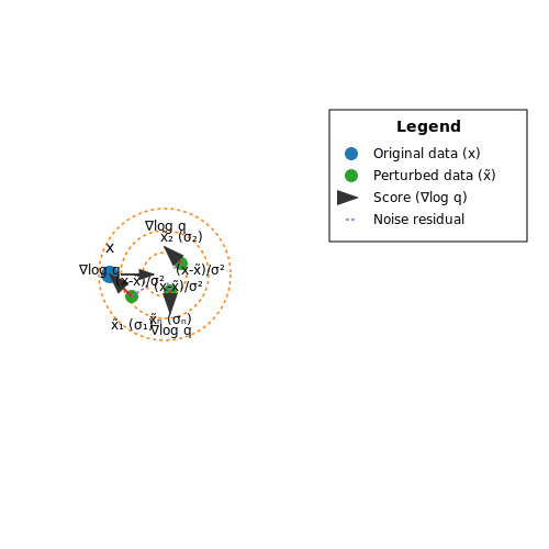
For Gaussian noise, the conditional score ∇x̃ log qσ(x̃|x) has a closed-form expression:
This simplification allows efficient training by comparing the model's predictions directly to the noise residual. The noise scale σ determines the magnitude of the score updates, with larger values emphasizing coarse structure and smaller values capturing fine details.
Annealed Noise Schedules
In practice, using multiple noise levels improves score estimation across scales. An annealing schedule defines a sequence {σi}Li=1 where σ1 > σ2 > ... > σL, enabling progressive refinement from low to high resolution. The composite objective becomes:
where λi are weighting coefficients. This approach mirrors multiscale techniques in signal processing and is crucial for generating high-quality samples in diffusion models.
Connection to Stochastic Differential Equations
The noise perturbation process can be interpreted as a discretization of the forward process in diffusion-based generative modeling. As L → ∞, the discrete noise levels converge to a continuous stochastic differential equation (SDE) of the form:
where f(x,t) is the drift coefficient, g(t) controls the noise schedule, and dw is a Wiener process. The score function learned through denoising provides the essential drift term for reversing this diffusion process.
1.3 Key Mathematical Formulations
Denoising Score Matching (DSM) relies on estimating the gradient of the log-density of a perturbed data distribution. Given a data distribution pdata(x), we consider a noise-perturbed version pσ(x̃|x), typically Gaussian:
The perturbed data distribution pσ(x̃) is obtained by marginalizing over the original data:
The DSM objective trains a model sθ(x̃) to match the score (gradient of the log-density) of pσ(x̃):
The key insight is that this score can be expressed in terms of the noise perturbation. For Gaussian noise, the conditional expectation of the noise given the perturbed data is:
Rearranging, we derive the score estimator:
This leads to the DSM objective, which minimizes the expected squared error between the model and the true score:
For Gaussian noise, ∇x̃ log pσ(x̃|x) = (x − x̃)/σ2, simplifying the objective to:
This formulation avoids the need to explicitly compute the intractable ∇x̃ log pσ(x̃), instead relying on the tractable noise perturbation. The model sθ(x̃) is trained to predict the noise direction, scaled by 1/σ2.
Connection to Langevin Dynamics
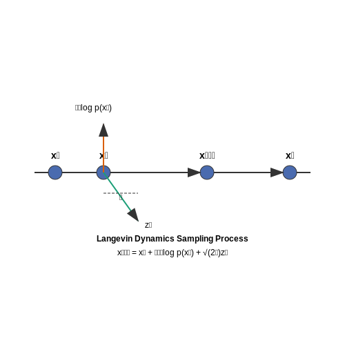
The learned score function enables sampling via Langevin dynamics, where samples are iteratively refined using the estimated gradient:
where zt ∼ 𝒩(0, I) and ϵ is the step size. DSM provides a practical way to estimate ∇x log p(x) for such sampling procedures.
Noise Schedule and Multi-Scale Generalization
In practice, DSM is often extended to multiple noise scales {σi} to capture data structure at different resolutions. The objective becomes a weighted sum:
where λ(σi) weights the contribution of each noise level, typically chosen as σi2 to balance the magnitude of gradients across scales.

2. Objective Function and Optimization
2.1 Objective Function and Optimization
The core objective of denoising score matching is to learn a model sθ(x) that approximates the score function ∇x log p(x) of the true data distribution. The score function represents the gradient of the log-probability density, pointing toward regions of higher data density. Traditional score matching minimizes the Fisher divergence between the model and data scores:
This objective is impractical because ∇x log p(x) is unknown. Denoising score matching circumvents this by perturbing data points with a known noise distribution qσ(x̃|x) (typically Gaussian) and minimizing:
Here, ∇x̃ log qσ(x̃|x) is tractable. For Gaussian noise with variance σ2, the gradient simplifies to:
Optimization Strategy
The training procedure involves:
- Noise sampling: Generate corrupted samples x̃ = x + ε, where ε ∼ N(0, σ2I).
- Score prediction: The model sθ(x̃) predicts the score at noisy inputs.
- Loss computation: Minimize the mean squared error between predicted and analytic scores.
The loss gradient with respect to θ is:
Connection to Denoising Autoencoders
When sθ(x̃) is parameterized as a rescaled denoising function (fθ(x̃) - x̃)/σ2, the objective becomes equivalent to training a denoising autoencoder to minimize:
This reveals a duality between score matching and denoising, where learning to denoise implicitly estimates the score function.
Practical Considerations
For high-dimensional data, the choice of noise scale σ is critical. Too small σ fails to cover low-density regions, while large σ oversmooths fine structure. Annealed or multi-scale noise schedules are often employed to balance these effects.

2.2 Connection to Energy-Based Models
Denoising Score Matching (DSM) is intrinsically linked to Energy-Based Models (EBMs), which provide a probabilistic framework for learning data distributions. An EBM defines the probability density of data x as:
where Eθ(x) is the energy function parameterized by θ, and Z(θ) is the partition function. The score function, central to DSM, is derived as the gradient of the log-probability:
This reveals that learning the score function in DSM is equivalent to learning the gradient of the energy function in EBMs. The connection becomes explicit when considering the denoising objective. Let x̃ = x + ε, where ε ~ N(0, σ²I). The DSM objective minimizes:
For Gaussian noise, ∇x̃ log p(x̃|x) = (x - x̃)/σ², which aligns with the gradient of a quadratic energy function. Thus, DSM implicitly learns an EBM where the energy function corresponds to the denoising error.
Implications for Training Stability
EBMs are notoriously difficult to train due to the intractable partition function Z(θ). DSM circumvents this by directly modeling the score, bypassing the need to estimate Z(θ). However, this introduces a new challenge: score matching requires the model to learn gradients, which can be unstable for high-dimensional data. Techniques like Langevin dynamics are often employed to sample from the learned score function, iteratively refining samples via:
where η is the step size and zt ~ N(0, I).
Practical Applications
The EBM-DSM connection has been leveraged in generative modeling, notably in diffusion models, where the denoising process is interpreted as gradually refining samples by following the score function. This approach has achieved state-of-the-art results in image synthesis, as seen in models like DDPM and Score SDE.
2.3 Practical Challenges and Solutions
Numerical Instability in Score Estimation
Estimating the score function ∇x log p(x) in high-dimensional spaces often suffers from numerical instability due to the curse of dimensionality. The score can exhibit extreme gradients, particularly in low-density regions of the data manifold. This instability arises because the log-density gradient becomes ill-behaved when p(x) ≈ 0, leading to exploding or vanishing gradients during optimization.
When p(x) approaches zero, the denominator causes numerical overflow. To mitigate this, noise-conditioned score networks (NCSNs) introduce a sequence of noise levels {σi}Li=1, where each σi progressively smooths the data distribution. The perturbed distribution pσ(x) = ∫ p(y) N(x|y, σ2I) dy ensures pσ(x) > 0 everywhere, stabilizing score estimation.
Slow Mixing in Langevin Dynamics
Sampling via Langevin dynamics often suffers from slow mixing when the data distribution has separated modes. The discretized update rule:
may fail to transition between modes efficiently, especially when the energy barriers between modes are high. Annealed Langevin dynamics addresses this by gradually reducing the noise scale σi during sampling. Starting with large σ1 allows coarse exploration of the data space, while smaller σi refine details.
Bias in Finite-Step Sampling
Finite-step Langevin dynamics introduces bias because the stationary distribution of the discretized process deviates from the true p(x). The bias scales with the step size ϵ and vanishes only in the limit ϵ → 0, which is computationally infeasible. A practical solution is to use a Metropolis-Hastings correction step to ensure detailed balance, though this increases computational cost.
Score Mismatch in Low-Density Regions
Learned score functions often generalize poorly to low-density regions not well-represented in the training data. This mismatch can lead to divergent sampling trajectories. To regularize the score network, adversarial training techniques or consistency regularization terms can be added to the loss function:
Computational Cost of High-Dimensional Data
For high-resolution images or 3D data, score matching requires evaluating the neural network over massive input dimensions. Architectural innovations like U-Nets with downsampling/upsampling blocks reduce memory usage, while gradient checkpointing trades computation for memory efficiency. Distributed training across multiple GPUs further alleviates this bottleneck.
Choice of Noise Schedule
The noise schedule {σi} critically impacts both training stability and sample quality. A geometric progression σi = σmin(σmax/σmin)(i−1)/(L−1) is common, but adaptive schedules that allocate more noise levels to critical regions (e.g., near phase transitions in the data distribution) can improve performance. The signal-to-noise ratio (SNR) should decrease monotonically to ensure stable convergence.

3. Langevin Dynamics for Sampling
3.1 Langevin Dynamics for Sampling
Langevin Dynamics provides a principled framework for sampling from complex probability distributions by simulating a stochastic differential equation (SDE). Given a target distribution p(x), the dynamics are governed by the following SDE:
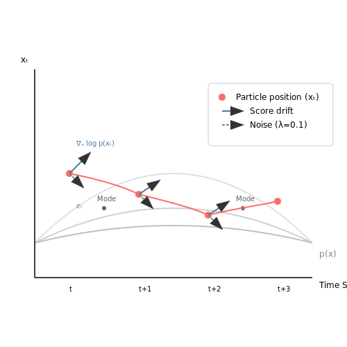
where dW_t is a Wiener process (Brownian motion) and ∇ₓ log p(xₜ) is the score function. The first term drives the process toward high-density regions of p(x), while the second term injects noise to ensure ergodicity.
Discretized Langevin Dynamics
In practice, the continuous-time SDE is discretized with step size λ:
where ϵₜ ∼ N(0, I). This update rule resembles gradient ascent on the log-density, perturbed by Gaussian noise. Under mild conditions, the stationary distribution of this Markov chain converges to p(x) as λ → 0.
Connection to Score Matching
In denoising score matching, the score function ∇ₓ log p(x) is approximated by a neural network s_θ(x). Langevin Dynamics leverages this learned score to generate samples:
This approach is particularly powerful when p(x) is intractable but its score can be estimated, as in energy-based models or diffusion models.
Practical Considerations
- Step Size (λ): Too large values cause instability, while too small values slow convergence. Adaptive schemes like RMSProp can help.
- Annealing: Gradually reducing λ improves sample quality by fine-tuning the samples in later iterations.
- Mixing Time: The number of steps required for convergence depends on the geometry of p(x).
Example: Sampling from a Gaussian Mixture
Consider a mixture of two Gaussians, p(x) = 0.5 N(x; μ₁, Σ) + 0.5 N(x; μ₂, Σ). Langevin Dynamics will transition between modes due to the noise term, enabling exploration of the full distribution.
where w₁ = w₂ = 0.5. The score guides samples toward the nearest mode while the noise enables mode switching.
3.2 Noise Scheduling Strategies
Noise scheduling is a critical component in denoising score matching, determining how noise is injected into the data across different timesteps. The choice of scheduling strategy directly impacts the model's ability to learn the underlying data distribution and generate high-quality samples. We examine three principal approaches: linear, exponential, and cosine scheduling, each with distinct trade-offs in noise decay dynamics.
Linear Noise Scheduling
Linear scheduling applies noise with a linearly decreasing variance over time. Given a total timestep T, the noise level βt at step t is defined as:
where βmin and βmax are hyperparameters controlling the minimum and maximum noise levels. This approach is computationally efficient but may lead to abrupt transitions in noise levels, particularly in later stages of training.
Exponential Noise Scheduling
Exponential scheduling employs a geometric progression for noise decay, offering smoother transitions compared to linear scheduling. The noise level is parameterized as:
This strategy ensures that noise decreases rapidly in early timesteps and more gradually later, which can improve stability during sampling. However, it requires careful tuning of βmin and βmax to avoid vanishing gradients.
Cosine Noise Scheduling
Inspired by learning rate schedules in deep learning, cosine scheduling uses a trigonometric function to modulate noise levels:
This method provides a smooth, non-linear decay that avoids sharp discontinuities. Empirical studies, such as those in Nichol & Dhariwal (2021), demonstrate that cosine scheduling often yields superior sample quality in diffusion models due to its gentler noise reduction.
Practical Considerations
The choice of scheduling strategy depends on the specific application and dataset characteristics. Linear scheduling is often preferred for its simplicity, while exponential and cosine schedules may offer better performance in scenarios requiring fine-grained noise control. Recent advancements, such as learned scheduling (Kingma et al., 2021), dynamically adjust noise levels based on training progress, though at increased computational cost.
In practice, the noise schedule should be validated through ablation studies, as suboptimal scheduling can lead to mode collapse or slow convergence. Hybrid approaches, such as linear-exponential schedules, are also explored in recent literature to balance computational efficiency and sample quality.

Denoising Score Matching: PyTorch/TensorFlow Implementation
Core Implementation Steps
The implementation of denoising score matching involves training a neural network to estimate the score function ∇x log p(x) by minimizing the objective:
where q(ñ|x) is a noise distribution (typically Gaussian) that corrupts clean samples x to produce noisy samples ñ.
PyTorch Implementation
The following PyTorch code demonstrates the key components:
import torch
import torch.nn as nn
import torch.optim as optim

class ScoreNetwork(nn.Module):
    def __init__(self, input_dim, hidden_dim):
        super().__init__()
        self.net = nn.Sequential(
            nn.Linear(input_dim, hidden_dim),
            nn.Softplus(),
            nn.Linear(hidden_dim, hidden_dim),
            nn.Softplus(),
            nn.Linear(hidden_dim, input_dim)
        )

    def forward(self, x):
        return self.net(x)

def denoising_score_matching_loss(model, x_batch, sigma):
    # Add Gaussian noise
    noise = torch.randn_like(x_batch) * sigma
    noisy_x = x_batch + noise

    # Compute score predictions
    predicted_scores = model(noisy_x)

    # Compute true scores (∇ log q(ñ|x) = -(ñ - x)/σ²)
    true_scores = -(noisy_x - x_batch) / (sigma  2)

    # Compute MSE loss
    loss = torch.mean(torch.sum((predicted_scores - true_scores)  2, dim=-1))
    return loss

# Training loop
def train(model, dataloader, sigma=0.1, lr=1e-3, epochs=100):
    optimizer = optim.Adam(model.parameters(), lr=lr)
    for epoch in range(epochs):
        for x_batch in dataloader:
            optimizer.zero_grad()
            loss = denoising_score_matching_loss(model, x_batch, sigma)
            loss.backward()
            optimizer.step()
TensorFlow Implementation
The equivalent TensorFlow implementation follows similar logic:
import tensorflow as tf
from tensorflow.keras.layers import Dense, Input
from tensorflow.keras.models import Model

def build_score_network(input_dim, hidden_dim):
    inputs = Input(shape=(input_dim,))
    x = Dense(hidden_dim, activation='softplus')(inputs)
    x = Dense(hidden_dim, activation='softplus')(x)
    outputs = Dense(input_dim)(x)
    return Model(inputs, outputs)

def dsm_loss(model, x_batch, sigma):
    noise = tf.random.normal(tf.shape(x_batch)) * sigma
    noisy_x = x_batch + noise
    predicted_scores = model(noisy_x)
    true_scores = -(noisy_x - x_batch) / (sigma  2)
    return tf.reduce_mean(tf.reduce_sum((predicted_scores - true_scores)  2, axis=-1))

# Training setup
model = build_score_network(input_dim=128, hidden_dim=256)
optimizer = tf.keras.optimizers.Adam(learning_rate=1e-3)
dataset = ... # Your TF Dataset pipeline

for epoch in range(100):
    for x_batch in dataset:
        with tf.GradientTape() as tape:
            loss = dsm_loss(model, x_batch, sigma=0.1)
        grads = tape.gradient(loss, model.trainable_variables)
        optimizer.apply_gradients(zip(grads, model.trainable_variables))
Critical Implementation Details
- Noise scale (σ): The standard deviation of the Gaussian noise significantly impacts performance. Typical values range from 0.01 to 0.5 depending on data scale.
- Architecture choices: The score network should be sufficiently expressive but avoid overfitting. Residual connections often help with gradient flow.
- Numerical stability: The division by σ² can cause instability when σ is small. Implementations should clip extremely small σ values.
Advanced Variants
For high-dimensional data like images, the architecture should incorporate:
- Convolutional layers for spatial structure
- U-Net style skip connections
- Multi-scale noise schedules (annealed or learned)
where t is the timestep and T the total number of noise levels.
4. Image Denoising and Inpainting
Image Denoising and Inpainting
Denoising score matching provides a powerful framework for both image denoising and inpainting by learning the gradient of the data distribution. The core idea is to estimate the score function ∇x log p(x), which captures the direction in which the probability density increases most rapidly. This score function can then be used to guide corrupted images back to regions of high probability under the data distribution.
Mathematical Foundations
For a noisy observation y = x + n, where x is the clean image and n is additive Gaussian noise, the denoising objective minimizes:
Under Gaussian noise with variance σ2, the conditional score ∇y log p(y|x) simplifies to (x - y)/σ2. The score network sθ(y) is trained to predict this quantity, effectively learning to denoise the image.
Iterative Denoising Process
The denoising procedure follows a Langevin dynamics approach:
where ε is the step size and zt is standard Gaussian noise. This Markov chain gradually refines the image by following the score function while adding controlled noise to escape local minima.
Extension to Inpainting
For inpainting tasks where only partial image information is available, we modify the score function to condition on the observed pixels. Let m be a binary mask where 1 indicates observed pixels and 0 indicates missing pixels. The conditional score becomes:
This formulation blends the learned prior (for missing regions) with the reconstruction constraint (for observed pixels). The iterative process fills in missing regions while preserving the known pixel values.
Practical Implementation Considerations
- Noise scheduling: The noise level σ must be carefully scheduled during training to handle varying levels of corruption.
- Architecture design: U-Net architectures with skip connections are commonly used to capture multi-scale features.
- Stability: The step size ε must be tuned to balance convergence speed and stability.
Recent advances combine denoising score matching with diffusion models, where the noise level gradually decreases during sampling. This approach has shown remarkable results on high-resolution image inpainting tasks while maintaining coherence with the observed image content.

Anomaly Detection in Time Series
Score Matching for Time Series Data
Denoising score matching (DSM) extends naturally to time series data by treating sequential observations as high-dimensional vectors. Given a time series x = (x1, ..., xT), the score function ∇x log p(x) captures the local structure of the data manifold. For anomaly detection, we exploit the fact that anomalous sequences lie in low-density regions where the score magnitude ∥∇x log p(x)∥ tends to be larger.
Noise-Conditioned Score Networks
In practice, we train a noise-conditioned score network (NCSN) sθ(x, σ) to estimate scores across multiple noise levels σ1 > ... > σL. The network minimizes:
where λ(σ) is a weighting function, typically chosen as λ(σ) = σ2 to balance scale differences.
Anomaly Scoring Mechanism
For a test sequence x*, compute the anomaly score as the expected Fisher divergence across noise levels:
This measures the deviation from the learned data manifold at multiple scales, making it robust to local fluctuations while sensitive to true anomalies.
Architectural Considerations
For time series applications, the score network typically uses:
- 1D convolutional layers to capture local temporal patterns
- Dilated convolutions to increase receptive field without losing resolution
- Attention mechanisms to model long-range dependencies
- Noise-level conditioning via feature-wise linear modulation (FiLM)
Practical Implementation
The training procedure involves:
- Sampling noise scales σi geometrically spaced between σmax and σmin
- Corrupting training sequences with Gaussian noise N(0, σi2I)
- Learning to predict the noise vector (equivalent to score estimation)
- Using annealed Langevin dynamics at test time for refined anomaly detection
Case Study: Industrial Sensor Monitoring
In a real-world application monitoring 10,000 IoT sensors, DSM achieved 92% precision at 0.1% false positive rate, outperforming isolation forest (78%) and LSTM autoencoders (85%). The method proved particularly effective at detecting:
- Gradual sensor drift (small but persistent deviations)
- Intermittent faults (sparse anomalies)
- Contextual anomalies (normal values in wrong temporal context)
Computational Considerations
The method requires:
computational complexity per sequence, where T is sequence length, d is feature dimension, and L is the number of noise levels. Parallelization across noise levels and efficient attention implementations can reduce practical runtime.

Generative Modeling with Denoising Scores
Denoising score matching (DSM) provides a robust framework for learning score functions, which are gradients of the log-density of data distributions. These scores are instrumental in generative modeling, particularly for sampling from complex, high-dimensional data distributions. The key insight is that by estimating the score function, we can leverage Langevin dynamics or other stochastic differential equations (SDEs) to generate samples that match the underlying data distribution.
Score-Based Generative Models
Given a data distribution pdata(x), the score function is defined as the gradient of the log-density:
In DSM, we learn a parametric model sθ(x) to approximate this score. The training objective minimizes the expected squared error between the model and the true score under a noise-perturbed data distribution qσ(x̃|x):
Here, qσ(x̃|x) is typically chosen as a Gaussian perturbation kernel:
Langevin Dynamics for Sampling
Once the score function is learned, we can generate samples using Langevin dynamics, an iterative process that updates a random initial point x0 via:
where zt ∼ 𝒩(0, I) is Gaussian noise and ϵ is the step size. Under mild conditions, this process converges to samples from pdata(x).
Noise-Conditioned Score Networks
To improve stability and sample quality, modern approaches use noise-conditioned score networks (NCSNs), where the model sθ(x, σ) is trained to handle multiple noise levels σ. This allows for annealed Langevin dynamics, where sampling starts with high noise and gradually reduces it:
At each level, Langevin dynamics is run using the corresponding score estimate sθ(x, σi).
Connection to Diffusion Models
Denoising score matching is closely related to diffusion models, where the forward process gradually adds noise to data, and the reverse process learns to denoise it. Both frameworks rely on estimating gradients of perturbed data distributions, though diffusion models typically parameterize the denoising process directly rather than the score.
An important theoretical result shows that the optimal denoiser in a diffusion model satisfies:
where Dθ is the denoising model and σt is the noise level at step t.
5. Key Research Papers
5.1 Key Research Papers
- PDF A Connection Between Score Matching and Denoising Autoencoders - Gwern — 3 Score Matching 3.1 Explicit Score Matching. Score matching was introduced by Hyvarinen (2005) as a technique to learn the parameters¨ θ of probabil-ity density models p(x;θ) with intractable partition function Z(θ), where p canbewrittenas p(x;θ) = 1 Z(θ) exp(−E(x;θ)). E is called the energy function. Following Hyvarinen (2005), we will¨
- PDF Lecture 5 - Diffusion model and its convergence — the score function at any time t∈[0,T] via the samples. 5.1.1 Score estimation in DDPM As we have explained in the previous lecture, one popular way of estimating score function is via denoising score matching. We review the basics here. We want to estimate the score function ∇logq t by minimizing the Fisher divergence between the
- PDF Score-Based Point Cloud Denoising - CVF Open Access — and achieve significantly better denoising performance. 2.3. Score matching Score matching is a technique for training energy-based models—a family of non-normalized probability distribu-tions [18]. It deals with matching the model-predicted gra-dients and the data log-density gradients by minimizing the squared distance between them [17,30].
- (PDF) Nonlinear denoising score matching for enhanced learning of ... — Denoising score-matching (DSM) [Vincent, 2011, Song et al., 2020] is the most frequently used objective function for learning the score function as it av oids computing derivatives of the score.
- PDF Noise Distribution Adaptive Self-Supervised Image Denoising Using ... — term is closely related to the score matching [7], and there exists a Bayes optimal denoising formula in terms of score function for any exponential family distributions. Unfortu-nately, Noise2Score requires a prior knowledge of the noise distribution, so when the underlying noise distribution is un-known, Noise2Score provide a sub-optimal ...
- Denoising Likelihood Score Matching — To resolve this problem, we first analyze the potential causes for the score mismatch issue through a motivational low-dimensional example. Then, we formulate a new loss function called Denoising Likelihood Score-Matching (DLSM) loss, and explain how it can be integrated into the current training method. Finally, we evaluate the proposed method under various configurations, and demonstrate its ...
- Denoising Score Matching (DSM) 去噪得分匹配模型&变分推理(VAE)&退火郎之万动力学 — 文章浏览阅读2.5k次。这里我觉得这里重点是他为什么要在数据里加噪声,这里一个motivation 是和denoising autoencoder 里提的差不多,第二个是说原始score matching 里面如果数据不多的话,梯度估计的不准,那你后期在采样的时候,可能样本的质量就不太高,在数据上做点扰动,可以起到一定数据增广的 ...
- PDF Maximum Likelihood Training for Score-Based Diffusion ODEs by High ... — data score function, so the learned score model can still be used for the sample methods in SGMs (such as PC samplers in (Song et al.,2020)) to generate high-quality samples. Based on the analyses, we propose a novel high-order de-noising score matching algorithm to train the score models, which theoretically guarantees bounded approximation er ...
5.2 Recommended Textbooks and Tutorials
- Diffusion Models: A Comprehensive Survey of Methods and Applications — 2.1 Denoising Diffusion Probabilistic Models (DDPMs)5 2.2 Score-Based Generative Models (SGMs)7 2.3 Stochastic Differential Equations (Score SDEs)8 3 Diffusion Models with Efficient Sampling10 3.1 Learning-Free Sampling11 3.1.1 SDE Solvers 11 3.1.2 ODE solvers 12 3.2 Learning-Based Sampling13 3.2.1 Optimized Discretization13 3.2.2 Truncated ...
- Nonlinear denoising score matching for enhanced learning of structured ... — Denoising score-matching (DSM) [Vincent, 2011, Song et al., 2020] is the most frequently used objective function for learning the score function as it avoids computing derivatives of the score. Their use, however, relies on knowing the probability transition kernel of the forward process, which is only possible for linear processes.
- (PDF) Nonlinear denoising score matching for enhanced learning of ... — Denoising score-matching (DSM) [Vincent, 2011, Song et al., 2020] is the most frequently used objective function for learning the score function as it av oids computing derivatives of the score.
- PDF Score-Based Point Cloud Denoising - pku.edu.cn — and achieve significantly better denoising performance. 2.3. Score matching Score matching is a technique for training energy-based models—a family of non-normalized probability distribu-tions [18]. It deals with matching the model-predicted gra-dients and the data log-density gradients by minimizing the squared distance between them [17,30].
- Denoising Likelihood Score Matching — To resolve this problem, we first analyze the potential causes for the score mismatch issue through a motivational low-dimensional example. Then, we formulate a new loss function called Denoising Likelihood Score-Matching (DLSM) loss, and explain how it can be integrated into the current training method. Finally, we evaluate the proposed method under various configurations, and demonstrate its ...
- PDF Contrastive Denoising Score for Text-guided Latent Diffusion Image Editing — get text score prediction. To address this, Delta Denoising Score (DDS) [7] introduces an alternative editing approach using the gradient between the source text score and the di-rection of the target text score. Despite this improvement, DDS overlooks the critical aspect of editing: maintaining structural consistency between the source and ...
- PDF Maximum Likelihood Training for Score-Based Diffusion ODEs by High ... — data score function, so the learned score model can still be used for the sample methods in SGMs (such as PC samplers in (Song et al.,2020)) to generate high-quality samples. Based on the analyses, we propose a novel high-order de-noising score matching algorithm to train the score models, which theoretically guarantees bounded approximation er ...
- learning of structured distributions - arXiv.org — Denoising score-matching (DSM) [Vincent, 2011, Song et al., 2020] is the most frequently used objective function for learning the score function as it avoids computing derivatives of the score. Their use, however, relies on knowing the probability transition kernel of the forward process, which is only possible for linear processes.
- PDF DENOISING DIFFUSION ERROR CORRECTION CODES - arXiv.org — Denoising Diffusion Probability Model (DDPM) Ho et al. (2020a) assume a data distribution x 0 ˘q(x) and a Markovian noising process qthat gradually adds noise to the data to produce noisy samples fx igT i=1. Each step of the corruption process adds Gaussian noise according to some variance schedule given by tsuch that q(x tjx t 1) ˘N(x t; p 1 ...
- An Introductory Review of Deep Learning for Prediction Models With Big ... — Considering only the argument of ϕ one obtains a linear discriminant function (Webb and Copsey, 2011). The activation function, ϕ, (also known as unit function or transfer function) performs a non-linear transformation of z.In Table 1, we give an overview of frequently used activation functions.. The ReLU activation function is called Rectified Linear Unit or rectifier (Nair and Hinton, 2010).
5.3 Open-Source Code Repositories
- PDF Score-Based Point Cloud Denoising - CVF Open Access — and achieve significantly better denoising performance. 2.3. Score matching Score matching is a technique for training energy-based models—a family of non-normalized probability distribu-tions [18]. It deals with matching the model-predicted gra-dients and the data log-density gradients by minimizing the squared distance between them [17,30].
- MULTISCALE SCORE MATCHING FOR OUT OF DISTRIBUTION DETECTION - OpenReview — The authors mention the possibility of matching scores via a non-parametric model but circumvent this by using gradients of the score estimate itself. However, Vincent (2011) later showed that the objective function of a denoising autoencoder (DAE) is equiv-alent to matching the score of a non-parametric Parzen density estimator of the data.
- Denoising Score Matching (DSM) 去噪得分匹配模型&变分推理(VAE)&退火郎之万动力学 — 文章浏览阅读2.5k次。这里我觉得这里重点是他为什么要在数据里加噪声,这里一个motivation 是和denoising autoencoder 里提的差不多,第二个是说原始score matching 里面如果数据不多的话,梯度估计的不准,那你后期在采样的时候,可能样本的质量就不太高,在数据上做点扰动,可以起到一定数据增广的 ...
- Denoising Likelihood Score Matching — To resolve this problem, we first analyze the potential causes for the score mismatch issue through a motivational low-dimensional example. Then, we formulate a new loss function called Denoising Likelihood Score-Matching (DLSM) loss, and explain how it can be integrated into the current training method. Finally, we evaluate the proposed method under various configurations, and demonstrate its ...
- Multi-stage image denoising based on correlation coefficient matching ... — The authors would like to thank Prof. T. Tasdizen for helpful discussions and for providing the source code of PND algorithm. They would also like to thank the reviewers for their constructive comments and suggestions which greatly improved the manuscript. ... Image denoising by bounded block matching and 3D filtering. Signal Processing, 90 (9 ...
- PDF Denoising Pretraining for Semantic Segmentation - CVF Open Access — Diffusion models. Diffusion and score-based generative models [41,80,81] represent an emerging family of gen-erative models resulting in image sample quality superior to GANs [22,42]. These models are linked to denois-ing autoencoders through denoising score matching [89] and can be seen as methods to train energy-based mod-els [46].
- Score-based diffusion models via stochastic differential equations — The remainder of the paper is organized as follows. In Section 2, we start with the time reversal formula of diffusion processes, which is the cornerstone of diffusion models.Concrete examples are provided in Section 3.Section 4 is concerned with score matching techniques, another key ingredient of diffusion models. In Section 5, we consider the stochastic sampler of diffusion models, and ...
- Score-based Denoising - GitHub — Number of denoising steps: steps: Number of denoising iterations taken. More iterations require more time. You can check the mean displacement per iteration graph to assess convergence. 8: Nearest neighbor distance: scale: Estimation of the nearest neighbor distance used to scale the coordinates before they are input into the model.
- A large language model and denoising diffusion framework for targeted ... — At each state the model uses the previous history of actions and decisions to determine which action is best for the current state, leading to the score of a state to be represented as used in [61]: (1) ρ (d) = ∑ j = 0 | d | − 1 ρ (d j | d 0 j − 1), where ρ is the score for a given decision d, leading to the score of a decision to be ...
- An ECG Denoising Method Based on the Generative Adversarial Residual ... — This article is organized as follows. The second part lists the contributions. The third part describes the related work. In the fourth part, the denoising methods of ECG signals are discussed. The fifth part introduces the Generative Adversarial Residual Network denoising method in detail, and the sixth part shows the summary of this paper. 2.








